Towards Agile Animated Characters

(1)

Proceedings of the 2000 IEEE International Conference on Robotics & Automation

San Francisco, CA • April 2000

Towards Agile A n i m a t e d Characters

M i c h i e l v a n de P a n n e J o e L a s z l o P e d r o H u a n g P e t r o s F a l o u t s o s D e p a r t m e n t o f C o m p u t e r S c i e n c e U n i v e r s i t y o f T o r o n t o *

A b s t r a c t

Dynamic simulation is a potentially useful tool for cre- ating realistic motion for animated characters. How- ever, improved control techniques are required before this approach will bear fruit. We compare and con- trast control for animation with control for robotics. This is followed by an overview of two control meth- ods which were conceived in the context of computer animation, but which also have potential applications for robotic control.

1

Introduction

Physically-based models and simulations are behind an increasing number of tools and techniques in computer graphics. Dynamic simulations are particu- larly well suited to generating passive motions, such as the movement of a character's clothing, the motion of falling and fracturing objects, and the motion of fluids. However, the simulation of human motions remains a formidable challenge given the many complexities involved in the simulation and control. Formidable accomplishments in this area have come from biomechanics[20], robotics[17, 22], and control[9]. The physically-based simulation of human motion is also of interest in computer animation[l, 2, 8]. Simulation-based animation techniques have also been used to generate realistic animated motion for more imaginary creatures[19, 23, 25]. At first sight it would appear that the use of a complex physical simulation is unwarranted when the end result is an animated motion that could just as well have been created di- rectly with a kinematic method. However, kinematic algorithms produce unconstrained motion trajectories

* {van, jflaszlo ,psh,pfal}@dgp.utoronto. c a

whose lack of a physical basis is often readily apparent. In production animations, the talents of an animator can be relied upon to edit the motions until they are sufficiently realistic. However, this is an impossibil- ity in the realistic interactive environments that many games and virtual worlds strive to provide.

The use of procedural kinematic algorithms[6, 5, 10] or, alternatively, playback of stored motion data captured from real human actors is currently the method of choice in some animation tools and many computer games, although such methods suffer from being lim- ited to the repertoire of captured motions. Algorithms to alter captured motions can be used to provide an expanded repertoire of motions and are a current topic of research in the animation community[7, 11]. Given the physical origins of the motions, it is perhaps not surprising that some of these motion transformation algorithms are reverting to the use of physics in order to compute plausbile transformations[21].

In many scenarios, it can be argued that a full-fledged physical simulation, together with the appropriate control algorithms, is the most compact representa- tion of a class of motion. Consider, for example, the difficulty of representing two colliding football players using only a set of stored motions examples. The difficulty of enumerating the large number of possible motions that can arise in such a scenario is evidenced in the current generation of games by the unrealistic motion often apparent during such events.

1 . 1 T h e A n i m a t i o n P e r s p e c t i v e

The task of intelligently controlling the motion of a simulated character has many similarities to the task of intelligently controlling the motion of a real robot. However, there are some notable differences between the animation problem and the robotics problem. As

(2)

well, there are many different variations on the animation control problem. The following list elaborates on some of the characteristic axes that define the design space for the motion control problem in animation.

Hard physics vs soft physics.

In creating an animation, a desired motion specification such as "leap 10m forward" might well be impos- sible. In the context of animation, this need not necessarily be a problem. A clever animation tool can relax the laws of physics just enough to allow the motion to be performed, resulting in a motion that satisfies the motion specification, while still being yielding a 'best fit' to the constraints imposed by physics. Alter- natively, animation tools can treat physics as a hard constraint, as implemented by a conventional forward dynamics simulation.

Observed motions vs synthetic motions.

The dynamics involved in creating a motion can be modelled either explicitly, as is the case with typical dynamic simulations, or implicitly, as is the case with good kinematic animation which nevertheless attempt to mimic the appropriate physics. While explicit models are perhaps the most interesting, given that they synthesize motion from first principles, implicit models have the advantage of being able to exploit data captured from real human motions. Motion capture technology has made such data increasingly available, and with the right techniques, captured motions can be generalized to produce novel motions.

Degree of autonomy.

Generating the motion of a foreground character in a feature film is a different problem from generating the motion of a character in a game. The former necessitates detailed control over the motion, while the latter must be capable of interactive autonomous motion. Such different applications are best served by tools uniquely tailored for each, given the different needs. For example, a game character requires models for sensing and planning in order to operate autonomously. These same skills are assumed by an animator when animating a feature-film character.

Visual quality vs. stability

In robotics and control, guarantees of stability are im- portant, while in animation the visual quality is of primary importance.

1 . 2 P r a c t i c a l C o n s i d e r a t i o n s

A number of practical considerations require attention when considering the use of dynamic simulations as a means for creating animation. First, the user interface

is necessarily of prime importance. Creating animated motions, whether through traditional animation techniques or using complex dynamic simluations, is a cre- ative process and thus the tools should be predictable in their actions, should provide suitable feedback, and should support the required workflow for creating an- imatious. This is no small challenge, given that these requirements are superimposed on top of already difficult control problems.

The use of physics in computer games presents a fur- ther interesting dilemna. Imagine that you are in control of a running character and you suddenly wish to execute a sharp turn to the right. A physically- realistic solution might require waiting until a particular phase in the stride where the sharp turn can be executed. However, from the game-player's per- spective, this lends a 'sluggish' feel to the game. The fidelity to physics must be compromised in order to accomodate the game-player's wishes.

Lastly, the computer graphics world is not bound by the conventional methodology used in robotics, namely that of treating control and simulation as two separate problems. For the purposes of animation, it may well be more efficient to build a model which en- compasses both dynamics and control, thus yielding a black box which accepts high-level motion commands as input and generates appropriate motions as output.

1 . 3

Explorations

Given the large body of literature which is relevant to the dynamic simulation of human-like characters and robots, it is beyond the scope of this article to provide an overview. Instead, the following two sections present two distinct approaches to control that are drawn from our own work, and which we feel provide useful insights relevant to both robotics and computer animation.

In section 2 we describe the use of limit cycle con-

trol as a general method for controlling the balance of

walking or running gaits. The technique is successfully applied to the control of a 3D dynamically-simulated walking gait, among others. Section 3 presents a technique for planning dynamic motions. The goal here is to provide motions with the anticipatory behavior necessary to execute very dynamic motions across variable terrain. While the results are demonstrated using physical systems having only a few degrees of freedom, they lend potential insight into the planning of dynamic motions. Lastly, conclusions are provided in section 5.

(3)

: : : : : : : : : : : : : : : : : : : : : : : : : : : : : : : : : .::- ~ : : ~ : : : ~ : ~ : : ~ : : : : : : : : : : : : : : : : : : : : : : : : : : : : : : : : : : .::::~...:.:,.,- . . . : ::::

Figure 1: T h e h u m a n model.

2

Limit C y c l e C o n t r o l

T h e dynamic simulation of h u m a n walking is a surprisingly difficult task, as evidenced by the assumptions and simplifications commonly used in the literature. T h e limit-cycle control algorithm described here is based upon existing ideas of limit cycle control[13, 18]. T h e instantiation we propose makes relatively few assumptions a b o u t the specifics of the gait and the anthropometry. T h e algorithm is capable of stabilizing walking gaits for dynamically-simulated h u m a n models, as well as particular running gaits. A complete description of the m e t h o d and the results can be found in [16].

T h e articulated skeleton used for our simulations has 19 degrees of freedom (DOF) and is shown in Fig- ure 1. T h e dimensions and physical p a r a m e t e r s have been chosen t o be a realistic reflection of measured h u m a n a n t h r o p o m e t r i c data. T h e character has two D O F ankle joints, t h r e e D O F hip joints, and one D O F joints elsewhere. A commercially available dynamics package[15] is used as the core of our simulation and is augmented with procedures for computing the internal and external forces. Internal forces (i.e., torques) are computed using the limit-cycle control algorithm to be described shortly; external ground-reaction forces are c o m p u t e d using a p e n a l t y - m e t h o d contact model. This contact model allows for slippage u n d e r the appropriate circumstances.

T h e point of departure for the control algorithm is a cyclic finite-state machine (FSM) which operates in a deterministic fashion. Each state has associ- ated parameters which specify a set of desired joint angles. T h e joint torques are t h e n c o m p u t e d using proportionai-derivative (PD) controllers, which drive the joints towards their desired configurations. State transitions occur after a fixed time duration, with the exception of two sensor-based transitions. These latter transitions are activated when the left and right feet strike the ground and their function is to keep the FSM synchronized with the movement in progress. Given a p p r o p r i a t e initial conditions and appropriate

choices of parameters, the FSM-based controller described thus far is sufficient t o make a simulated h u m a n take several walking or running steps before falling over due to a lack of balance. T h e goal of the limit cycle control mechanism is t o introduce small control p e r t u r b a t i o n s into t h e FSM, which will serve t o provide the balancing actions.

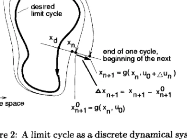
T h e operation of the limit-cycle control is illustrated in an a b s t r a c t fashion in Figure 2. T h e loop drawn in bold gives the desired periodic motion of the sys- t e m state. T h e goal of the controller will be to push the system s t a t e back onto this trajectory. Instead of dealing with the continuous system dynamics, however, we can significantly simplify m a t t e r s by creating a discrete dynamical system. This is done by sampling the motion once per cycle, as illustrated in the figure. T h e discrete dynamical system can t h e n be expressed as xn+l = g ( x n , u n ) , where xn is the system state at the s t a r t of cycle n, xn+l is the system state at the end of cycle n, un represents the control inputs applied during cycle n, and the function g is the state transition function. If the original FSM-based controller provides control inputs u0, t h e n the limit cycle controller must c o m p u t e the control p e r t u r b a t i o n ~ u n such t h a t the applied control, un = u0 + Aun, results in the state returning t o the desired limit cycle, i.e.,

X n . J c l ~ X d .

In order to f u r t h e r simplify the problem, we introduce the use of a reduced-order model for the system dynamics. First, we note t h a t balance is concerned with avoiding a fall, and thus the basic requirement for Xd is t h a t the simulated h u m a n be upright at the end of each step. T h e r e are several ways of defining upright; one of the simplest is to a t t a c h an up vector to the coordinate frame of the pelvis. By projecting the up vector onto the ground plane, we obtain two compo- nents, one which measures tilt in the lateral plane, i.e., to the left or right, and a n o t h e r which measures tilt in the sagittal plane, i.e., forwards or backwards. We refer to these two observable p a r a m e t e r s as the regula- tion variables, as we wish t o drive the values of these variables to zero, or some o t h e r suitably-chosen t a r g e t values.

An appropriate choice of control variables is required to effect the desired control over the regulation variables. T w o control variables are required in order to yield a controllable system. Several choices are possible; one robust choice we use is to apply an additive p e r t u r b a t i o n to the t a r g e t hip angles in one or more of the FSM states. This affects t h e sagittal and lateral pitch of the t r u n k segment during the motion and thus can serve as a mechanism for balance control.

(4)

d ,\

end ot one cycle, beginning o! the next x n + 1 = g( x n , u 0 + ~ u n ) , ~ X n + l = Xn+ 1 - xnO+l

state s p a c e xnO+ 1 = g( Xn' Uo )

Figure 2: A limit cycle as a discrete dynamical system.

I I I f I I I I J S / I f I

I ? I I I I I I 1 / I I I J

Figure 3: Simulated movements for a human model and robot.

Given the definition of the 2D discrete dynamical system, the control algorithm constructs a first order model of the state transition function, g, by evaluating the Jacobian, ~ at state xn. This is done once for each simulated walking step, using a total of four simulations of the same step, each executed with different control parameters. Finite differences are then used to construct the linear model.

Figure 3 illustrates two variations on a human walk as well as a running gait synthesized for a bird-like robot. Animations of these motions are available on the web[24]. The speed, direction, and style of the walks can be controlled independently of the balancing mechanism. Subjectively speaking, the walks exhibit a rather robotic style, although we intend to explore tuning mechanisms capable of producing more natu- ral walks. Based on the results to date, however, the limit-cycle control algorithm is of potential interest for both animation and robotics applications.

Figure 4: A Flipping Acrobot.

3 Planning Dynamic Motions

The synthesis of regular, periodic gaits such as walking and running is only a starting point for developing the types of dynamic motions which are readily observable in soccer players, tennis players, or cross-country runners. These sports require novel actions that are beyond the scope of a parameterized gait controller and they typically involve interaction with unstruc- tured dynamic environments. In such scenarios, it is difficult to make a distinction between planning and control. Fundamental questions to be asked about such motions include What action vocabulary is ap- propriate ]or planningf and How far ahead should one

plan ? To this end, we have experimented with a finite-

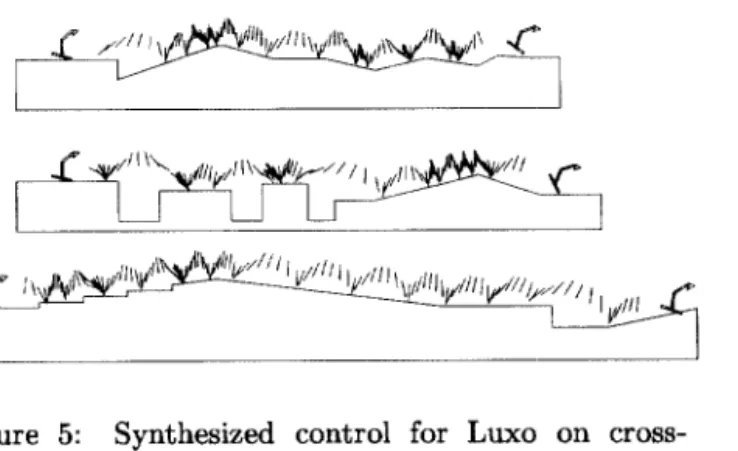
horizon planning algorithm, tested on simplified 'creatures' which are never the less capable of very dynamic motions[14]. One of our creatures is the acrobot, a two- link underactuated robot which has been the subject of considerable study in the control literature[12, 3, 4]. Our goal will be to create a sequence of animted flips, as shown in Figure 4. The other is Luxo, a 'jumping lamp,' drawn from a computer animation context. We shall explain the motion planner by way of an example. Figure 5 shows the output of the motion planning algorithm for the jumping lamp character. This is a planar articulated figure consisting of three links connected by two single-DOF joints. The problem to be solved is the same for each of the four terrain seg- ments: find the sequence of control actions necessary for Luxo to hop across the terrain in minimal time and without falling. For clarity, Figure 5 only illustrates the motion of the middle link. The final motions, view- able on the web[24], exhibit considerable anticipation of the upcoming terrain, which we shall argue is both realistic and desireable.

The motion planning process is carried out as follows. Luxo is given discrete repertoire of five control actions, which we shall denote as a, b, c, d, and e. Each of these actions corresponds to a different variation of a forward 'hop.' Qualitatively, these hops vary in their

(5)

///ll\vl~

Figure 5: Synthesized control for Luxo on cross- country runs.

wastefully planning too far ahead. The current control decision should be influenced by the shape of the terrain up to four jumps ahead, which is a surprisingly long planning horizon.

The same motion planning algorithm also allows for explorations of the capabilities of particular dynamical systems. In particular, we consider the acrobot,

a simple two-link articulated figure which has a single DOF actuated joint. Novel motions can be synthesized by using the finite-horizon planning process with an objective function which measures progress towards a desired behavior. For example, we have produced control strategies which allow the acrobot to perform sequences of cartwheels, front flips, back flips, and forward balanced hopping. An example of a back-flip sequence is shown in Figure 4. These animations are also available online[24].

amounts of forward or backward lean. All the hops are implemented using a three-state FSM with fixed, timed state transitions. Each state provides a unique set of desired joint angle values, which are used by local PD controllers on each joint in order to produce the internal torques which drive the motion.

As output, the planning algorithm should produce the sequence of actions which causes Luxo to traverse the terrain in minimal time, e.g., d,a,b,b,c,a, .... This is done using a finite-horizon decision tree, which works as follows. A decision tree is constructed to explore the outcome of every possible action sequence of length n, where n represents the planning horizon. For our example, we have chosen n = 4, which leads to the simulation of 54 possible outcomes. The optimal decision sequence is then chosen based upon the final amount of progress made, i.e., the maximal distance travelled. The planner then commits to the first action of the optimal decision sequence. The entire process is repeated for each subsequent decision. While the decision tree grows exponentially as a function of the depth, this behavior is not seen in practice because of the early termination of branches due to falls, as well as the application of branch-and-bound techniques. One of the insights to be gained from the resulting motions is a meaningful evaluation of the required planning horizon for particular classes of motion. The variation of the measured performance, i.e., the time taken to traverse the terrain, can be plotted as a function of the planning horizon used, n. For the examples shown in Figure 5, there are no increasing returns to be had for n > 4. An optimal choice of n = 4 looks far enough ahead to achieve the best result, while not

4

C o n c l u s i o n s

The dynamic simulation of human motion is a common goal of computer animation, biomechanics, control systems, and robotics. Indeed, these respective fields of research already share many common tools and ideas, although they may differ in their end goals and their means of evaluating success. However, the largely disjoint publication forums for these areas still leaves room for improved collaboration and exchange in order to remove the artifacts t h a t arise from the academic partitioning.

We have described two control techniques which have potential implications for the dynamic simulation of human motion. Limit cycle control illustrates a general method for stabilizing simulated human walks and has the promise of extending to other types of gaits and anthropometry. The finite-horizon motion planner provides insight into the types of motions a dynamical system is capable of, as well as quantifying the amount of anticipation necessary for particular classes of motion.

R e f e r e n c e s

[1] N. I. Badler, B. Barsky, and D. Zeltzer. Making

Them Move. Morgan Kaufmann Publishers Inc.,

1991.

[2] N. I. Badler, C. Phillips, and B. Webber. Simu- lating Humans: Computer Graphics, Animation,

(6)

[3] M. D. Berkemeier and R. S. Fearing. Control of a two-link robot to achieve sliding and hopping gaits.

Proceedings, IEEE International Confer-

ence on Robotics and Automation,

pages 286-294,

1992.

[4] S. A. Bortoff.

Pseudolinearization Using Spline

Functions with Application

to the Acrobot.

PhD thesis, University of Illinois at Urbana- Champaign, 1992.

[5] R. Boulic, N. M. Thalmann, and D. Thalmann. A global human walking model with real-time kinematic personification.

The Visual Computer,

6:344-358, 1990.

[6] A. Bruderlin and T. W. Calvert. Goal-directed

animation of human walking.

Proceedings of

ACM SIGGRAPH,

23(4):233-242, 1989.

[7] A. Bruderlin and L. Williams. Motion signal pro- cessing.

Proceedings of Siggaph '95, ACM Com-

puter Graphics,

pages 97-104, 1995.

[8] J. K. Hodgins et al. Animating human athletics.

Proceedings of SIGGRAPH '95, ACM Computer

Graphics,

pages 71-78, 1995.

[9] Vukobratovic et al.

Biped Locomotion: Dynam-

ics, Stability, Control and Applications.

Springer

Verlag, 1990.

[10] M. Girard. Interactive design of computer-

animated legged animal motion.

IEEE Comptuer

Graphics and Applications,

7(6):39-51, June

1987.

[11] Michael Gleicher. Retargeting motion to new characters.

Proceedings of SIGGRAPH 98,

pages 33-42, July 1998. ISBN 0-89791-999-8. Held in Orlando, Florida.

[12] J. Hanser and R. M. Murray. Nonlinear controllers for non-integrable systems: the acrobot example.

Proceedings, American Control Confer-

ence,

pages 669-671, 1990.

[13] H. M. Hmam and D. A. Lawrence. Robustness analysis of nonlinear biped control laws via sin- gular perturbation theory.

Proceedings of the 31st

IEEE Conference on Decision and Control,

pages

2656-2661, 1992.

[14] P. S. Huang and M. van de Panne. A search algorithm for planning dynamic motions.

Computer

Animation and Simulation '96,

pages 169-182,

September 1996.

[15] Symbolic Dynamics Inc.

SD/Fast User's Manual.

1990.

[16] Joseph F. Laszlo, Michiel van de Panne, and Eu- gene Fiume. Limit cycle control and its application to the animation of balancing and walking.

Proceedings of SIGGRAPH 96,

pages 155- 162, August 1996.

[17] Honda Motor Co. Ltd. www.honda.co.jp /en-

glish/technology]robot/.

[18] T. McGeer. Passive dynamic walking.

The Inter-

national Journal of Robotics Research,

9(2):62-

82, 1990.

[19] J. T. Ngo and J. Marks. Spacetime constraints revisited.

Proceedings of SIGGRAPH '93,

pages 343-350, 1993.

[20] Marcus G. Pandy and Frank C. Anderson. Three- dimensional computer simulation of jumping and walking using the same model. In

Proceedings of

the VIIth International Symposium on Computer

Simulation in Biomechanics,

1999.

[21] Zoran Popovic and Andrew Witkin. Physically

based motion transformation.

Proceedings of

SIGGRAPH 99,

pages 11-20, August 1999.

[22] M. H. Raibert.

Legged Robots that Balance.

MIT Press, 1986.

[23] U. Sims. Evolving virtual creatures.

Proceed-

ings of SIGGRAPH '94, A CM Computer Graph-

ics,

pages 15-22, 1994.

[24] M. van de Panne. Animations web page.

http ://www. dgp. utoronto, ca/'van/ani, html.

[25] M. van de Panne and E. Flume. Sensor-actuator networks.

Proceedings of SIGGRAPH '93,

pages 335-342, 1993.