Essays on Rational Asset Pricing.

(1)

(2)

(3)

Essays on Rational Asset Pricing

Proefschrift

ter verkrijging van de graad van doctor aan de Univer-siteit van Tilburg, op gezag van de rector magnificus, prof. dr. F.A. van der Duyn Schouten, in het openbaar te verdedigen ten overstaan van een door het college voor promoties aangewezen commissie in de aula van de Uni-versiteit op maandag 18 december 2006 om 16.15 uur door

Marta Szymanowska

(4)

(5)

Preface

Parts of the research reported in this dissertation are written in cooperation with others. Chapters 2 and 4 are written with Frans de Roon. Chapter 3 is based on a paper with Rob van den Goorbergh, Theo Nijman and Frans de Roon. Chapter 5 originated from joint work with Jenke Ter Horst and Chris Veld.

Acknowledgements

While writing this thesis I have been guided and supported by numerous people. Frist and foremost, I would like to thank my supervisor Frans de Roon for his guidance. I have benefited tremendously from his knowledge, insight and experience. Also, I would like to thank Frans for providing encouragement (sometimes very much needed) and for the confidence he had in me (always very much needed). Thank you Frans!

I am also deeply indebted to my supervisors Jenke Ter Horst and Chris Veld. We worked together in the early stage of my Ph.D. track, they helped me make my first steps in research and taught me academic thinking and writing. I have greatly appreciated their keen involvement in supervising me. I would like to thank Jenke (who had an office just next door) for being open to all my questions and concerns and for helping me get through the troubles of the life of a Ph.D. student.

I would also like to thank other members of my committee, Lieven Baele, Frank de Jong, Geert Rouwenhorst (Yale School of Management), and Marno Verbeek (Erasmus University Rotterdam), for their willingness to participate in the Ph.D. committee and for giving valuable advices on the thesis.

Many thanks to my colleagues and friends Anna, Chendi, Crina, Harald, Marina, Mark-Jan, Michaela, Norbert, Simon, and Valentina for making my life at Tilburg Uni-versity scientifically challenging and stimulating, and outside the uniUni-versity filling it with fun, adventures, sports, and Culture. I am very happy that I met you! Special thanks to Marie for helping me out with the Dutch summary. I am also grateful to my friends back

(6)

home Ada, Aneta and Michal, Kasia, and Monika who always knew that one supporting word I was looking for, and made the distance between Tilburg and Krak´ow bearable. I hope I was able to express my gratitude to all of you during our contacts either directly or via emails.

Last but definitely not least I want to express my deepest appreciation towards my family. Maciek, there are no words that would come close to being able to express my gratitude and happiness that you have supported and believed in me, and eagerly participated in our exciting finance-marketing discussions. Being my husband you are also my best friend and my best colleague! Finally, I want to thank my parents and my sister who taught me how to live and always supported my choices - even when it led me to live abroad.

Marta Szymanowska Tilburg, August 2006

(7)

Chapter 1

Introduction

This thesis consists of four essays that deal with rational asset pricing. If agents have rational expectations,1 the most fundamental asset pricing equation states that there exists a pricing kernel or stochastic discount factor mt+1 such that for the excess return ri,t+1 on any asset or security, we have

Et[mt+1ri,t+1] = 0, (1.1)

i.e., the conditional expectation of the excess returns multiplied by the stochastic dis-count factor equals zero. One way to interpret this stochastic disdis-count factor is to think that mt+1 generalizes the standard discounting idea, i.e. it incorporates all risk

correc-tions into one variable, and the asset specific correccorrec-tions are generated by the covariance between the random component of this common stochastic discount factor and asset specific payoff. Another interpretation of the pricing kernel is that it is the marginal utility of the investor, i.e. mt+1 measures the rate at which investors are willing to trade

consumption at time t for consumption at timet+ 1.

Equation (1.1) implies that the expected excess return on any security or asset de-pends on the covariance of the security return with the pricing kernel

Et[ri,t+1] =−

Covt[ri,t+1, mt+1] Et[mt+1]

. (1.2)

The expected return on any security or the risk premium is larger, the more negative is the covariance of a security return with the pricing kernel. Such assets deliver low returns in bad states of the economy, hence investors require more compensation for holding them. On the contrary, investors desire securities that deliver high payoffs in

1_{Assuming markets are frictionless and the law of one price holds.}

(12)

these bad states. This means that investors prefer assets that covary positively with the pricing kernel and such assets will have lower expected returns or risk premiums.

The first essay of this thesis: Consumption Risk and Expected Futures Returns, fo-cuses on the unconditional and conditional implications of Equation (1.1) and applies them to the cross-section of expected futures returns. Understanding these futures returns, whose expectations basically reflect risk premia, is important for academics studying asset pricing models as well as for practitioners, since they are important input variables for portfolio and risk management models e.g. More specifically, in this essay we focus on a relation between expected futures returns and a pricing kernel that is im-plied by a consumption-based asset pricing model. In this context, the pricing kernel is measured by the intertemporal marginal rate of substitution (IMRS) of a representative investor that is a function of only the growth rate in aggregate per capita consumption. If Equation (1.1) holds unconditionally, then unconditional expected returns are linear in one factor only (i.e. a standard unconditional Consumption CAPM prevails), and if Equation (1.1) holds conditionally, then for the unconditional expected returns a two factor unconditional model is obtained. Not only securities with higher consumption risk have higher unconditional expected returns (CCAPM), but also securities that have consumption betas that vary more with the market risk premium.

This standard consumption-based framework appears to be the most preferable, at least from a theoretical point of view. First, because it accounts for the intertemporal nature of the portfolio decision (Merton (1973), Breeden (1979)). Second, because it implicitly incorporates many forms of investors’ wealth (not only stock market wealth) that are relevant for measuring systematic risk of assets (Mankiw and Shapiro (1986), Cochrane (2001)). Despite the theoretical appeal of the consumption-based model, em-pirical studies have not been successful in applying it to the cross-section of stock returns (Campbell and Cochrane (2000)). This problem has been addressed by a recent stream of literature, which focuses on the underlying assumption that investors can costlessly adjust their consumption (Jagannathan and Wang (2005), Parker and Julliard (2005)). We follow up on this research by applying it to a broader set of assets than stocks only. We use futures contracts that have as the underlying assets various commodities (agriculturals, meats, energy and precious metals) as well as currencies and an equity index. We study whether excess returns on futures contracts vary in a systematic way due to differences in consumption risk similarly to the returns on stocks. Historically, commodity futures have earned excess returns similar to those of equities (Gorton and Rouwenhorst (2006)), nevertheless they fulfill a different economic function. Moreover,

(13)

3

since the underlying commodities are strongly related to aggregate consumption itself and may be used for hedging consumption risk, these futures markets seem to be a nat-ural choice for testing consumption-based model. Finally, Lewellen, Nagel, and Shanken (2006) show that the tests of the asset pricing models based on the Fama-French size and book-to-market portfolios are often misleading, as these portfolios are known to have a strong factor structure, i.e. high time-series and cross-sectional predictability based on the Fama-French factors. Hence the use of futures returns, representing a separate asset class, only strengthens our tests.

We find that the Consumption CAPM explains up to 60 percent of the cross-sectional variation in mean futures returns. The conditional version of the consumption model performs best at the quarterly horizon and outperforms both the CAPM and the Fama-French three-factor model. We show that expected futures returns can be measured by the futures’ yields and that the consumption model, next to explaining mean returns, is also best at explaining the cross-sectional variation in mean yields. Unlike for stock returns, ultimate consumption (i.e., contemporaneous plus future consumption) leads to lower performance of the consumption model. We show that demand and supply changes lead short term consumption risk to be important for commodities, but not long term consumption risk. We find that consumption betas measured with respect to the ultimate consumption growth fade out to zero and the consumption model controlling for the changes in production better explains the cross-section of futures returns. This suggests that for commodities we observe an impact of supply on commodity prices and therefore on consumption inducing time-varying consumption betas, whereas for stock markets the link between the supply (of stocks) and consumption is not to be expected. Thus, to the extent that commodity price changes are followed by changes in demand and supply, this may explain why ultimate consumption risk is not as good a risk measure for commodities as for stocks.

The second essay: An Anatomy of Commodity Futures Returns: Time-varying Risk Premiums and Covariances,assumes that Equation (1.1) holds conditionally and focuses on the time-series behavior of expected commodity futures returns. First, we decom-pose expected futures returns in the spot and term premiums. This decomposition is important, because the two risk premiums are likely to compensate for different risk factors (e.g. for oil futures the spot premium reflects the oil price risk, while the term premium mainly reflects the risk that is present in the convenience yields). We show that although average returns in commodity futures markets are claimed to be zero, the spot and term premiums that define them have opposite signs and both premiums are

(14)

highly predictable. We are able to predict up to 30 percent of the time-variation in these risk premiums, with the spot premium being more predictable than the term premiums. This knowledge allows investors to design trading strategies that exploit these different premiums and their predictable variation.

The documented time-variation in expected futures returns or risk premiums is an-alyzed and confronted with three asset pricing models: the CAPM, the Fama-French three-factor model and the Consumption CAPM. We find that this predictability seems to be consistent with the consumption-based model but not with the CAPM or the Fama-French model. In other words, predictability documented in futures markets is consistent with the exposure to consumption risk that an investor is undertaking while following a trading strategy that exploits predictability, but not to the market risk or risks re-lated to the Fama-French three factors. Since in the consumption-based model the risk of an asset is determined by its covariance with consumption growth, the time-varying expected returns should result from the time-varying conditional covariances between futures returns and consumption growth as follows from Equation (1.2). Indeed, we find that these covariances vary considerably over time. Consistent with the Breeden (1980) argument that the consumption betas of commodities may depend on their supply and demand elasticities, we find production growth to have stronger forecasting power for the conditional covariances than for futures returns.

The third essay: Predictability in Industry Returns: Frictions Matter, focuses in more detail on the predictability of asset returns and its relation to the asset pricing models. Following the work of Kirby (1998) we show that Equation (1.1) imposes restrictions on the slope coefficients and R2_s _{in predictive regression. In other words, predictability}

observed in the market must be consistent with the exposure to systematic risk that a rational investor is undertaking while following a trading strategy that exploits pre-dictability, i.e. the profits from that trading strategy must be equal to a risk premium implied by the asset pricing model. It is well recognized that the ability to predict returns can exist in efficient markets, but what yet remains a puzzle is whether this predictability is rational. Kirby (1998) finds that in frictionless markets asset pricing models are not able to generate levels of predictability observed in the market. It may very well be the case though, that the profits documented in the literature are not at-tainable for the investor because of the market frictions present in the real world. The inability to go short or the presence of transaction costs may force investors to deviate from the trading strategy that aims to exploit predictability in the market, which may alter their profits. Hence, it is important to incorporate these deviations when assessing

(15)

5

the rationality of trading strategies that track predictability.

The aim of this essay is to investigate the impact of the market frictions on the tests of the consistency of asset pricing theory with observed return predictability. We show how the restrictions derived by Kirby (1998) change when we take into account market frictions, such as short sales constraints and transaction costs. Incorporating short sales constraints weakens these restrictions. When the actual effect of some instruments is weaker in the market than suggested by the model, rational investors are willing to short sell these assets. However, being prohibited from doing so, investors might not be able to equate their profits with rational risk premiums. Thus, the asset pricing model with shorts sales constraints is only rejected when investors are over-compensated for true risk exposure. When we take into account transaction costs the restrictions are again weaker than in the frictionless markets, i.e. the higher the transaction costs, the weaker the restrictions. Moreover, in this case we are able to test to which extent transaction costs can reconcile predictability in financial markets, by deriving a threshold value for the transaction costs for which the coefficients from predictive regressions satisfy these weaker restrictions.

Futures markets can be assumed to be almost frictionless, which however, would be a very strong assumption for many other financial markets. Hence, we assess the impact of market frictions on the time-series behavior of asset returns by studying industry portfolios created from stocks traded in the major U.S. markets. We find strong evidence of return predictability among these industry portfolios, i.e., we can explain between 15 and 20 percent of return variance. Moreover, investors can enhance their investment opportunity set by adding active industry returns to the initial set of passive industry returns only, as they offer higher Sharpe ratios and higher risk-adjusted returns (relative to the factor models).

The results suggest that not taking into account market frictions may lead to in-correct conclusions. In frictionless markets, the documented predictability of industry returns does not seem to be consistent with rational asset pricing models, meaning that investors may be able to profit from the observed predictability more than what they expect to earn based on their exposure to risk. However, we find that these profits are only attainable if investors are able to trade without any costs. Transaction costs below 50 basis points are sufficient to reconcile much of the documented predictability. Furthermore, we find that a mean-variance investor significantly overstates his utility gain from return predictability that is not consistent with asset pricing models. When we incorporate market frictions these gains are substantially reduced.

(16)

Finally, in the last essay of this thesis: Behavioral Factors in the Pricing of Financial Products, we relax the assumption of rational asset pricing. In rational models agents are assumed to maximize their expected utility using identical probability beliefs for future states of the economy. We allow for behavioral biases on the side of the investor that may violate these assumptions and hence Equation (1.1).

In the last chapter we allow for these biases to explain mispricing that is observed in a particular class of securities, reverse convertible bonds. These are bonds that carry high coupon payments and in exchange, the issuer has an option at the maturity date to either redeem the bonds in cash, or to deliver a pre-specified number of shares. These bonds are mainly bought by individual investors who are not aware of the options, usually keep bonds in their portfolio and do not trade on the stock exchange, hence may be more prone to behavioral biases (i.e. may deviate from the behavior as suggested by rational asset pricing theory). We find that, on average, the plain vanilla RCs are overpriced by approximately 6%, while the knock-in RCs seem to be priced fairly. The documented overpricing seems to be driven by the option component. It is confirmed in a model-free analysis and is persistent for approximately one fourth of the lifetime of the reverse convertibles. Moreover, the documented overpricing remains significant in each year within our sample period. Given that the number of issuances increased over the sample period, this shows considerable economic losses to the investors in this market. Using a financial experiment in which we ask the participants to price a simple financial product with similar characteristics as a reverse convertible bond, we are able to test the role of behavioral factors like framing and cognitive errors, in explaining the documented overpricing. By showing that these factors are important we shed some light on the conclusion that the rational factors alone are not sufficient to explain the overpricing. Such an approach overcomes the difficulty (or even impossibility) in enumerating all possible rational explanations. We find that framing and cognitive errors, play an important role in the pricing of the simple financial product. Although the simple financial product is not exactly similar to a reverse convertible, our results shed some light on the ability of framing the redemption and the past stock price behavior to affect the pricing of the reverse convertible bonds.

(17)

Chapter 2

Consumption Risk and Expected

Futures Returns

2.1

Introduction

Futures returns are like excess returns on assets such as stocks and bonds, whose expec-tations basically reflect risk premia. Understanding these risk premia is important for academics studying asset pricing models as well as for practitioners, since they are im-portant input variables for portfolio and risk management models e.g. The determinants of futures risk premia are usually related to systematic risk based on the CAPM1 or the Consumption CAPM (CCAPM) as in Jagannathan (1985). Although Jagannathan (1985) finds for three different agricultural futures contracts that the CCAPM implies significant risk premia and finds market prices of risk that are similar to those found in equity markets, he rejects the model itself. Breeden (1980) studies a similar model on a broader class of commodity futures and finds significant consumption betas but he does not perform a full test of the asset pricing model. The evidence proclaimed so far in the empirical literature, indicates that although commodity returns appear not to be related to the movements in stock market returns,2 _{they do seem to be related to the}

changes in aggregate real consumption. The latter finding may be natural since part of the underlying commodities are strongly related to aggregate consumption itself and

1_{See, e.g., Dusak (1973), Black (1976), Carter, Rausser, and Schmitz (1983), Bessembinder (1992),}

and de Roon, Nijman, and Veld (2000).

2_{This is based on the unconditional version of the CAPM. However, futures contracts do exhibit}

systematic risk once betas are allowed to vary (e.g., Carter, Rausser, and Schmitz (1983)) and when, additionally, SMB and HML factors are included (e.g., Erb and Harvey (2006)).

(18)

may be used for hedging consumption risk. Hence, the consumption-based framework seems to be a natural choice for analyzing futures returns.

Previous studies find that the CCAPM has more difficulties in explaining the cross-section of stock returns than other models like the Fama-French three factor model (see Campbell and Cochrane (2000) and references therein).3 This problem has been ad-dressed by a recent stream of literature which focuses on the underlying assumption that investors can costlessly adjust their consumption plans. For instance, Jagannathan and Wang (2005) propose that consumption and investment decisions are made infre-quently and show that the CCAPM explains more than 70 percent of the cross-sectional variation in expected stock returns when consumption growth is measured from the 4th quarter of one year to the next. Also, they find that lowering the frequency of con-sumption growth and returns from monthly to quarterly and annual data, significantly improves the performance of the CCAPM, which is likely to result from the smaller mea-surement error in consumption growth at lower frequencies. Parker and Julliard (2005) conjecture that consumption may be slow to respond to stock returns, and find that ultimate consumption risk, defined as the covariance of a stock return and consumption growth over the quarter of the return and many following quarters, explains between 44 and 73 percent of the cross-sectional variation in stock returns.

This chapter follows up on the aforementioned advances in the literature on the CCAPM by applying them to a broad cross-section of 25 different futures contracts. We study whether excess returns on futures contracts vary in a systematic way due to dif-ferences in consumption risk similarly to the returns on stocks. Historically, commodity futures have earned excess returns similar to those of equities (Gorton and Rouwenhorst (2006)). Nevertheless, they fulfill a different economic function than corporate securi-ties such as stocks, i.e. they do not represent claims against future cash flows of the firm, but bets on the future expected spot prices of commodities. They also constitute a broader class of assets than simply stock returns, since they have as the underlying assets various commodities (agriculturals, meats, energy and precious metals), as well as currencies, bond and equity indices. The CCAPM may be particularly relevant to com-modity futures as commodities are closely linked to consumption and production factors.

3_{A second difficulty for the CCAPM is that it cannot explain the time-series average of stock returns,}

i.e., the high equity premium. In response to this, several refinements of the model have been put

forward. These models focus on better ways of modeling investors preferences. For example, the

model of Bansal and Yaron (2004) which uses the recursive utility preference of Epstein and Zin (1989, 1991) , or the Campbell and Cochrane (1999) model which allows for a habit formation in the utility specification; appear to be successful in solving these puzzles.

(19)

2.1. Introduction 9

Moreover, there are important differences between the consumption betas in stocks and in futures markets. First, for (commodity) futures it is common to observe positive as well as negative consumption betas, a feature less common in equity markets. Second, the contemporaneous consumption beta for longer maturity futures is usually lower than for shorter maturity futures (Breeden (1980)), which suggests that the time period over which consumption risk is measured may play an important role in determining the con-sumption risk in futures markets, unlike in stock markets. Finally, Lewellen, Nagel, and Shanken (2006) show that tests of the asset pricing models based on the Fama-French size and book-to-market portfolios are often misleading, as these portfolios are known to have a strong factor structure, i.e. high time-series and cross-sectional predictability based on the Fama-French factors. Hence the use of futures returns, representing a sep-arate asset class, only strengthens our tests.

We find that, at the quarterly horizon, the (unconditional) CCAPM explains about 50 percent of the cross-sectional variation in mean futures returns, while there is almost no explained variance at the monthly level, and an intermediate result at the yearly level. This pattern is consistent with the results found by Jagannathan and Wang (2005) based on stock portfolios. However we find somewhat lower implied consumption risk premi-ums for our futures contracts. When we assume that the model holds in a conditional sense (as in Jagannathan and Wang (1996)), allowing for time-varying betas and risk premiums, the CCAPM explains up to 60 percent of the cross-sectional variation in futures returns and again shows the best performance at the quarterly and annual fre-quency. In both cases, the consumption-based model explains the futures returns better than our benchmark models: the CAPM or the Fama-French model. As in previous empirical studies the CCAPM does show a high implied risk aversion though.

Using ultimate consumption risk as in Parker and Julliard (2005), we find that the performance of the CCAPM is best using consumption growth of the contemporaneous quarter of the returns, but then deteriorates for the longer horizons. Although this contradicts the findings of Parker and Julliard (2005) for stock returns, it is consistent with the finding that the CCAPM performs best at the quarterly frequency and may be the result of supply and demand elasticities of many of the commodities that un-derlie our futures contracts, inducing time-varying consumption betas. Indeed, we find that there are systematic decreases in the absolute values of the consumption betas of our commodities as the horizon, over which consumption growth is measured, increases. Consistent with the conjecture that production adjusts to changes in commodity prices but only slowly, we find that the variation in commodity returns explained by the

(20)

invest-ment growth model first increases with the measureinvest-ment horizon, and then decreases. A similar pattern is observed when we estimate the consumption model controlling for changes in production. This suggests that for commodities we observe an impact of supply on commodity prices and therefore on consumption inducing time-varying con-sumption betas, whereas for stock markets the link between the supply (of stocks) and consumption is not to be expected. Thus, to the extent that commodity price changes are followed by changes in demand and supply, our results may explain why ultimate consumption risk is not as good a risk measure for commodities as for stocks.

Finally, using a simple present value relation, we show that the futures’ own yield can be used as an estimator of expected returns similar to the way dividend yields are estimators of expected stock returns (see, e.g., Campbell and Shiller (1988) and Bekaert and Harvey (2000)). The futures’ yield has the advantage over the simple mean return that it is an ex ante measure of expected returns, while the mean return is an ex post measure. Using the average yield as the dependent variable in the cross-sectional regression, confirms that the CCAPM performs best at the quarterly frequency. However, the model can explain only up to 29 percent of the cross-sectional variation in yields in the unconditional case and up to 36 percent in the conditional case. The Fama-French model explains the cross-sectional variation in yields better (up to 45 and 58 percent respectively), but yields negative estimates of the market risk premia.

The rest of this chapter is structured as follows. The next section gives a brief outline of the unconditional and the conditional CCAPM. Section 2.3 discusses some estimation issues and Section 2.4 describes the data. The empirical results are discussed in Section 2.5 and Section 2.6 concludes.

2.2

Theory: Expected futures returns and

consump-tion risk

2.2.1

Consumption-based models for expected returns

According to finance theory, expected returns on securities are determined by their exposure to systematic economy wide risk. Rubinstein (1976) and Breeden (1979) show that the risk of a security is determined by its covariance with consumption growth (CCAPM). In this framework, a representative agent allocates her resources among consumption and different investment opportunities in order to maximize her utility

(21)

2.2. Theory: Expected futures returns and consumption risk 11

over lifetime consumption:

E " _∞ X s=t δsu(Cs) ! |Ft # , (2.1)

where we assume a time and state separable Von Neumann-Morgenstern utility function

u(·),Cs denotes consumption expenditures in periods,δis the time discount factor, and

Ft denotes the information set available to the representative agent at time t. The first

order conditions of the agent’s maximization problem subject to the standard budget constraints imply the following relation that is satisfied by all financial securities:

Et δju 0₍_C t+j) u0₍_C t) ri,t+j = 0 (2.2)

where ri,t+j is the excess return on any securityi,from datettot+j,u0(·) denotes first

derivative of the period utility function, and Et[·] denotes the expectation conditioned

on the information available at time t.

2.2.2

The unconditional Consumption CAPM

In the empirical analysis we work with both the unconditional and conditional versions of (2.2). We start with the unconditional model. Defining the stochastic discount factor (SDF) as mt+j ≡δj u0(Ct+j) u0₍_C t) gives: E[mt+jri,t+j] = 0 ⇐⇒ E[ri,t+j] =− Cov[ri,t+j, mt+j] E[mt+j]

where the second equality follows from using the definition of covariance and by applying the law of iterated expectations. Defining the sensitivity of excess returns ri,t+j to

changes in the stochastic discount factor as βic,j = Cov_{V ar}[ri,t_[_m+j,mt+j]

t+j] and the market price of

risk λc =−

V ar[mt+j]

E[mt+j] we get

E[ri,t+j] =λcβic,j. (2.3)

This is the standard beta representation of the unconditional Consumption CAPM. Expected excess returns on different securities are determined by their covariances with the stochastic discount factor, and thus by their covariances with consumption. A security with greater consumption risk has a higher expected return, since consumption

(22)

and marginal utility are inversely related. Later on we also consider other specifications for the stochastic discount factor implied by the CAPM (i.e. the SDF linear in the market return only) and by the Fama-French three factor model (i.e. the SDF linear in three risk factors: market, size and book-to-market).

2.2.3

The conditional Consumption CAPM

To model the implications of the conditional version of Equation (2.2):

Et[ri,t+j] =λ0c,t+λ1c,tβic,t, (2.4)

for the unconditional expected returns, we follow Jagannathan and Wang (1996). First, take unconditional expectations of (2.4):

E[ri,t+j] =λ0c+λ1cβic+Cov[λ1c,t, βic,t] (2.5)

whereβ_ic =E[βic,t] andλ1c =E[λ1c,t]. Then, projectingβic,t on the conditional market

risk premium λ1c,t, gives:

βic,t =βic+ϕic(λ1c,t−λ1c) +ηic,t (2.6)

with E[ηic,t] = E[ηic,tλ1c,t] = 0. Finally, substituting (2.6) into (2.5) gives for the

un-conditional expected returns:

E[ri,t+j] = λ0c+λ1cβic+V ar[λ1c,t]ϕic, (2.7)

ϕic =

Cov[λ1c,t, βic,t]

V ar[λ1c,t]

.

Thus, the conditional CCAPM leads to a two-factor unconditional model, in which the second factor is a risk premium induced by the covariance between the conditional beta βic,t and the conditional market risk premium for consumption risk λ1c,t.Not only

securities with higher expected betas have higher unconditional expected returns, but also securities with betas that vary more with the risk premium have higher uncondi-tional expected returns, i.e. a positive covariance implies that if βic,t is high when λ1c,t

is high, which will result in higher unconditional expected returns.

The conditional model expressed in this way requires estimation of the expected beta,

β_ic and the sensitivity of the conditional beta to the risk premium,ϕic,which cannot be

(23)

2.2. Theory: Expected futures returns and consumption risk 13

to the changes of the stochastic discount factor and the average reaction to the changes of the risk premium. This leads to the following unconditional betas:

βic ≡ Cov[ri,t+j, mt+j] V ar[mt+j] , (2.8) βiϕ ≡ Cov[ri,t+j, λ1c,t] V ar[λ1c,t] .

Jagannathan and Wang (1996) show that ifβiϕ is not a linear function ofβic, then there

exist some constants a0, a1, a2 such that for every security i the unconditional expected

return is a linear function of the above two unconditional betas:

E[ri,t+j] =a0+a1βic+a2βiϕ. (2.9)

We only summarize the idea of the proof here, for details see Appendix 2.A or the proof of Theorem 1 in Jagannathan and Wang (1996). First it is shown that when betas vary over time, then (βic, βiϕ) is a linear function of (βic, ϕic), which follows from additional

assumptions about the residual term from projection equation ηic,t. Second, when βiϕ

is not linear in βic (i.e. when the single beta CCAPM does not hold unconditionally,

even though it holds conditionally), then (βic, βiϕ) will contain all necessary information

contained in (β_ic, ϕic). Hence, expected returns will be linear in (βic, ϕic) as well as in

(βic, βiϕ).

2.2.4

Ultimate Consumption Risk

Recently, Parker and Julliard (2005) find that contemporaneous consumption risk, as in the models discussed in the previous sections, is not sufficient to explain the cross-section of stock returns. They propose to extend the contemporaneous measure with the subsequent time periods to account for possible slow consumption adjustment. To see this, let us rearrange the terms in (2.2) in the following way:

Et[u0(Ct+j)ri,t+j] = 0.

Combining the above with the Euler equation for the risk-free rate between time t+j

and t+j+S: Et+j h δu0(Ct+j+S)R_tf₊_j,t₊_j₊_S i =u0(Ct+j),

(24)

gives the following representation for expected returns: E[ri,t+j] = λc,Sβic,S, (2.10) βic,S = Cov ri,t+j, mSt+j V ar mS t+j , mS_t₊_j = δRf_t₊_j,t₊_j₊_Su 0₍_C t+j+S) u0₍_C t) , where CovmS t+j, ri,t+j

for large S is referred to as ultimate consumption risk and the market price of this risk is λc,S =−

V ar_[mS

t+j]

E_[mS

t+j]

.

We apply this approach to measure consumption risk in futures contracts. However, there are important differences between the consumption betas in stocks and in futures markets. First, for futures it is common to observe positive as well as negative consump-tion betas, a feature less common in equity markets. Second, as Breeden (1980) shows, the contemporaneous consumption beta for longer maturity futures is usually lower than for shorter maturity futures, due to supply responses. He argues that for short time-to-maturity futures, supply and demand elasticities may be assumed to be relatively small. As the time-to-maturity increases supply responses start to affect consumption-betas. This suggests that the time over which the consumption risk is measured will play an important role in determining the consumption risk in futures markets.

2.3

Estimation issues

This section presents the estimation issues. We, first, discuss the estimation of the stochastic discount factor and the sensitivity of futures returns to changes in this stochas-tic discount factor. Second, we discuss the estimation of the expected futures returns.

2.3.1

Estimating the CCAPM

We use the two stage cross-sectional regressions (CSR) approach with standard errors corrected for the estimation error in the dependent variable and for the fact that β0s

are pre-estimated as suggested by Fama and MacBeth (1973), Shanken (1992), and Jagannathan and Wang (1996). Moreover, since our sample consists of return histories that differ in length, we apply the procedure of Stambaugh (1997) to compute the multivariate moments without discarding any observations. The validity of the models is examined by testing whether Jensen’s alphas are zero (see Appendix 2.B for details).

(25)

2.3. Estimation issues 15

To parameterize the consumption-based model we assume that the period utility function has a constant relative risk aversion γ. This implies the following for the stochastic discount factor:

mt+j =δj ct+j ct −γ , where Ct+j Ct −γ

is the period-j growth in per capita consumption from time t to time

t +j. Given the above representation of the SDF, expected returns are a non-linear function of consumption growth. In the following, we assume that consumption growth and security returns are jointly log-normally distributed, which implies that the expected excess returns are linear in log-consumption growth:

E[ri,t+j] + 0.5V ar[ri,t+j] =γCov[ri,t+j,∆ct+j], (2.11)

where ∆ct+j ≡log

_C

t+j

Ct

.The above can be also expressed in the following beta repre-sentation: E[ri,t+j] = λ0+λcβic,j, (2.12) βic,j = Cov[ri,t+j,∆ct+j] V ar[∆ct+j] .

where the implied coefficient of relative risk aversion isγ = λc

V ar[∆ct+j]and the intercept is

λ0 =−0.5V ar[ri,t+j]. A similar beta representation can be obtained, without the need

to assume log normality but by using a Taylor series approximation of the stochastic discount factor around expected consumption growth.

In order to account for possibly slow consumption adjustment the log-consumption growth is measured over an extended horizon:

∆cS_t₊_j = log Ct+j+S Ct . (2.13)

See Appendix 2.C for details on the derivations. In addition, the conditional model re-quires observations on the conditional market risk premiumλ1c,t.We follow the approach

of Jagannathan and Wang (1996) utilizing the fact that a variable that helps predict the business cycle can also forecast the market risk premium. The logic behind this is based on the presumption that if prices vary over the business cycle, so might the market risk premiums. The empirical research on predictability has identified several potential variables, from which the most widely used are: a dummy for the January effect; a credit risk premium defined as the difference in yields between Moody’s Baa rank bonds and Moody’s Aaa rank bonds; a term structure premium defined as the difference between

(26)

90 days and 30 days Treasury Bill rate; a dividend yield on the S&P 500 index; and the return on the market index (see, e.g., Kirby (1998), Pesaran and Timmermann (1995), and Ferson and Harvey (1991)). Based on previous studies we use a term structure variable r_tterm₊₁ .4 Assuming that the market risk premium is linear in the conditioning variable, i.e. λ1c,t=b0+b1rtterm+1 , we can estimate the following conditional model:

E[ri,t+j] = λ0+λ1βic+λtermβi,term (2.14)

βic ≡

Cov[ri,t+j,∆ct+j]

V ar[∆ct+j]

,

βi,term ≡

Covri,t+j, rtterm+j

V arrterm t+j

.

2.3.2

Yield-based measure for expected returns

Traditionally, expected returns are measured as the averages of past returns. However, the estimates of means are sensitive to the number of observations and volatility of the return series (Merton (1980)). In this section we show that a present value model implies the use of yields as an alternative measure of expected returns. The futures’ yield has the advantage over the mean return that it is an ex ante measure of expected returns, while the mean return is an ex post measure.

To see the relation between commodity prices and yields we start from a simple present value model.5 _Define _P

t to be the spot price of a commodity, and Dt to be a

benefit from having the commodity available, i.e. the convenience yield net of storage and insurance costs. Later in the empirical section next to commodity futures we also use financial futures. For index futuresPt is the index, andDtare dividends (analogously to

common stocks); for foreign currency futuresPtis the spot price of the currency, andDt

are the interests payments from a foreign deposit. Then, the net return on a commodity from period t to period t+ 1 is:6

Rt+1 =

Pt+1−Pt+Dt

Pt

. (2.15)

Assuming that the expected returns are constant, i.e. Et[Rt+1] =µand Dt is expected

to grow at a constant rate g gives a standard Gordon-growth model for a commodity

4_{We also experimented with other predictive instruments, but our results are robust with respect to}

the choice of the instrument.

5_{A similar approach is used by Pindyck (1993).}

6_{Notice that the definition of a commodity return that is used here differs from commonly used}

commodity returns, Rp,t+1 =Pt+1/Pt−1, which consist of price changes only. Similar to total stock

(27)

2.3. Estimation issues 17

spot price:7

Pt =

Dt

µ−g,

whereµ > g. This relation implies that we can measure expected returns on commodities as the sum of the cash yields and growth rate in convenience yields:

µ= Dt

Pt

+g. (2.16)

Dynamic versions of this approach are used by Bekaert and Harvey (2000) e.g. For many commodities, the growth rate g is - at least in the long run - close to zero, at least in real terms. If the growth rate for commodities is indeed close to zero, then it follows immediately from (2.16) that the cash yield measures the expected total return on commodities. We test this presumption below. Thus, next to the standard way of estimating expected returns using historical averages we have an alternative measure based on yields.

A natural way to estimate yields is to use the information that is present in futures prices. DefineF_t(n)to be the commodity futures price for delivery at timet+n.Assuming that the cost-of-carry model holds, we have:

F_t(n) = Ptexp{−y (n) t ×n}, (2.17) f_t(n) = pt−n×y (n) t ,

where pt = log (Pt), ft = log (Ft) and y

(n)

t is the per-period yield for maturity n. By

a no arbitrage argument, this yield is equal to the net cash yield (i.e. the cash flow Dt

expressed as the percentage of price: st=dt−pt) minus the n-period interest rate:

y_t(n)=s_t(n)−i(_tn). (2.18) In general, this net cash yield,s(_tn), consists of the benefits that the owner of the security receives from holding the security from time t to time t+ 1 minus the costs of holding (storing) the security during the same period. For commodity futures the convenience yield constitutes the benefits from having a commodity available, while the cost of carrying the commodity to the future involves interest costs, physical storage costs, and insurance premiums. For financial futures there are no storage costs and the benefits from keeping the underlying asset are for instance the foreign interest rate for currency futures and the dividend yield for stock index futures.

7_{Additionally, we need to assume that the expected discounted value of the stock price K periods}

from the present shrinks to zero as the horizon K increases, which will be satisfied unless the stock price is expected to grow forever.

(28)

Then, a one-period log futures return, r_f,t(1)₊₁, can be decomposed in the following way: r_f,t(1)₊₁ = pt+1−f (1) t =pt+1−pt+y (1) t (2.19) = pt+1−pt+s (1) t −i (1) t =rt+1−i (1) t

Thus, the one-period futures return,r(1)_f,t₊₁, is like an excess return on the total commod-ity return, rt+1. Therefore, adding the one-period interest rate i(1)t to (2.19), taking the

expectations of both sides, and using the log version of (2.16) we get:

Ehr(1)_f,i,t₊₁+i(1)_t i =st+g, (2.20)

with st = dt−pt. Thus, using the assumption that the growth rate g is zero, we can

relate futures returns to yields in the following way:

r_f,i,t(1) ₊₁+i(1)_t =ai+bis(1)i,t +ei,t+1. (2.21)

Subtracting the one-period interest rate i(1)_t from both sides gives

r(1)_f,i,t₊₁ =αi+βiy

(1)

i,t +εi,t+1. (2.22)

At each point in time the expected one-period futures return is proportional to the per-period yield for the same one-per-period. Equation (2.22) shows that it is very natural to relate futures returns to yields if the growth rate in convenience yields is indeed zero.

Table 2.1 tests the presumption of zero growth rates in convenience yields for our dataset of 25 futures contracts (described in detail in Section 2.4). From (2.17) the per-period yields (yn

t) are computed as the log price differences between the

nearest-to-maturity contracts and the ones that are closest to having a maturity 12 months longer than the nearest-to-maturity contracts correcting for the varying length of spread. Then, from (2.18) the convenience yields are computed by correcting the yields with the interest rate over the same maturity. Finally, the table reports the average growth rates in convenience yields, their standard errors and the t-statistics for testing the significance of means. The results suggest that these growth rates are insignificantly different from zero, although this conclusion should be interpreted with caution since the standard errors are rather high.

Given that the estimated growth rates are insignificant, we expect a strong relation between the two measures for expected returns: return- and yield-based measure. Fig-ure 2.1 depicts the cross-sectional relation between the annualized average log returns

(29)

2.4. Data 19

on the nearest-to-maturity futures contracts, and the corresponding annual log yield. The plotted lines represent fitted values from the following cross-sectional regression of mean futures returns on mean yields:

rf,i=α+βyi+ui. (2.23)

The solid line depicts results from a regression with an intercept and the starred line from the regression without an intercept. This figure shows a strong, positive relation between mean returns and yields. This is confirmed by the high estimated R2 _{of the}

the above regression: 61.3% of the cross-sectional variation in mean returns is explained by the cross-sectional variation in mean yields. The results are reported in Table 2.2. The estimated intercept α_b is insignificantly different from zero and is equal to 2.6% per annum (with a standard error of 1.7%). When β in the cross-sectional regression is restricted to be one, then the intercept is equal to 2.5% pa with a standard error of 1.6%. This estimate of 2.5% can be interpreted as the average growth rate in yields over all 25 futures contracts (i.e., the average of the growth rates reported in Table 2.1), which confirms the presumption of zero growth rate in futures yields despite the high standard errors reported earlier. The estimated βb is in both cases (when we force an

intercept to be zero and not) within two standard errors from one. When we do not impose restrictions on the intercept βbis equal to 1.09 (with a standard error of 0.38),

and when we force an intercept to be zero, it decreases to 0.88 (with a standard error of 0.39).

2.4

Data

2.4.1

Futures data

We use data on 25 futures contracts that are obtained from the Futures Industry Institute (FII) Data Center. The starting date of our sample period varies between contracts, as we use all available information for each futures contract. The earliest starting date is February 1968. The end date, December 2004, is common for all series. Hence the number of observations varies between futures contracts in our sample.

The data can be divided into 20 commodity futures contracts and five financial futures contracts.8 The commodities comprise grains (3), oil and meals (3), meats (4), energy (3), precious metals (4), and food and fiber (3). The financial contracts consist

(30)

of an equity index (1) and foreign currencies (4). These markets have relatively large trading volumes and provide a broad cross-section of futures contracts. Details about the delivery months, the exchanges where these futures contracts are traded and the starting dates for each contract are given in Table 2.3.

As outlined in Section 2.3.2, our dependent variable - the expected return - is mea-sured in two ways: based on returns and yields. Futures returns are calculated using a rollover strategy of nearest-to-maturity futures contracts. Until the delivery month, we assume a position in the nearest-to-maturity contract. At the start of the deliv-ery month, the position is changed to the contract with the following delivdeliv-ery month, which then becomes the nearest-to-maturity contract. Prices of futures observed in the delivery month are excluded from the analysis to avoid irregular price behavior that is common during the delivery month. Depending on the delivery dates during the year, the different series are for delivery one to three months apart. We obtain a minimum of 194 and a maximum of 442 observations.

The second measure of expected returns, derived from the present value model, is based on futures yields. To avoid the problems of seasonal fluctuations in futures (convenience) yields, yearly yields are used. We construct the series of annual yields as the log price difference between the nearest-to-maturity contracts and the ones that are closest to having a maturity 12 months longer than the nearest-to-maturity contracts. Depending on the series, the maturities vary between 7 to 13 months. To correct for the varying length of the spread, we use yields projected on the maturity equal to exactly 12 months.

Descriptive statistics are presented in Table 2.4. Panel A describes the returns on 25 futures markets. The first three columns give the annualized mean returns computed for different frequencies. Consistent with previous studies9 _{we find that except for a few}

futures contracts (S&P 500, crude oil, unleaded gasoline and live cattle futures) the es-timated mean returns are statistically indistinguishable from zero at the 5% significance level. The highest average returns - more than 10% on an annual basis - are earned by energy futures. For some futures, e.g., soybean oil, cotton, coffee, and copper, we observe large differences in mean returns across the different frequencies of the data. Finally, the last column gives the annualized yields for different futures. The table shows that the cross-section of mean yields is smoother than of mean returns. For instance, the dispersion between the minimum and the maximum yield is smaller than for the mean

9_{See. e.g., Bessembinder (1992), Bessembinder and Chan (1992), and de Roon, Nijman, and Veld}

(31)

2.4. Data 21

returns.10

2.4.2

Consumption data

It is a well known fact that reported consumption data are subject to measurement problems. Theory implies that consumption risk is measured with respect to aggregate consumption growth between two points in time. In practice, however, we observe total expenditures on goods and services over a period of time. This creates a so called ”sum-mation (or time-aggregation) bias” (e.g., Breeden, Gibbons, and Litzenberger (1989)).

One way to avoid this problem is to use higher frequency consumption data. On the other hand, high frequency consumption data are measured less precisely, which may lead to less reliable (less stable) estimates. The higher frequency data may ex-hibit seasonal patterns, which might be especially important among the returns on commodity futures.11 _{Moreover, recent work by Jagannathan and Wang (2005) shows}

that consumption-risk measured with lower frequency data, can better explain the cross-section of the 25 Fama-French portfolios. Since establishing which of the aforementioned biases dominate in futures markets remains an empirical issue, we use monthly, quarterly and yearly consumption data in our empirical tests.

Following the literature, we measure consumption growth as the percentage change in the seasonally adjusted, aggregate, real per capita consumption expenditures on non-durable goods and services. We use monthly, quarterly and annual consumption and population data from the National Income and Product Accounts (NIPA) tables in Sec-tion 2 on Personal Income and Outlays. The sample period is dictated by the availability of futures prices, as the consumption data at all frequencies are observed at a longer time interval.

Panel B of Table 2.4 gives the descriptive statistics for the log consumption growth. The consumption growth during our sample period is slightly above 2% per annum

10_{We sometimes observe rather extreme returns, usually related to specific events. One example is}

the silver bubble in the turn of 1979. By the early 1970s silver began to rise in price, along with gold, platinum, oil, inflations and U.S. interest rates. The Commodities Futures Trading Commission falsely attributed the rise in silver prices to the market manipulations and changed the trading rules (i.e., margin requirements were raised to 100%, only futures sell orders were allowed), which lead to a collapse of the silver bubble. This is reflected in our data, where we observe almost 300% annual return for silver in 1979. In general we observe more volatility in the futures data, which is reflected in rather high standard deviations reported earlier. Since, these are inherent features of futures data we do not exclude any observations.

(32)

for all frequencies. Monthly consumption exhibits the highest growth and the highest volatility.

Benchmark factors

For the benchmark models we use two standard models: the CAPM and the Fama-French three-factor model. Since futures contracts are in zero net supply they do not enter the market portfolio, hence the CAPM also holds in economies where not only stocks but also futures are traded (de Roon, Nijman, and Veld (2000)). It remains an empirical question though, whether the two additional factors (size and book-to-market) improve the cross-sectional predictability of futures returns (see, e.g., Erb and Harvey (2006)). The standard benchmark research factors are retrieved from Kenneth French’s online data library. As these data are only available on a monthly and an annual basis, we compute quarterly returns by compounding monthly returns. Panel C of Table 2.4 gives the descriptive statistics for the benchmark factors, which confirms their standard features. In contrast to the mean futures returns given in Panel A, benchmark factors mean returns do not vary substantially across different frequencies.

2.5

Empirical analysis

2.5.1

Unconditional consumption risk

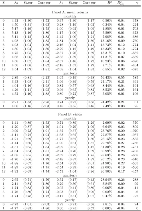
We start our empirical analysis with the unconditional version of the CCAPM in Equa-tion (2.3). Table 2.5 provides the cross-secEqua-tional estimates of λ0 and λc, based on our

25 futures contracts. Panel A reports the regression estimates for betas estimated at different frequencies: monthly, quarterly and yearly. Estimating beta at a monthly fre-quency leads to a very poor performance of the consumption model. The R2 of the cross-sectional regression is 2.5%, and the market price of consumption risk is not sig-nificantly different from zero.

At lower frequencies, the CCAPM fares much better: for quarterly estimates, the

R2 increases to 51% and for yearly estimates it is 35%. As in Lewellen, Nagel, and Shanken (2006) the 95% confidence intervals for the true R2 are rather wide though, which may result from the use of only 25 cross-sectional observations. Nevertheless, the lower bounds are always above zero for the unadjusted R2_s. _{A similar pattern shows}

up for the benchmark models: all models have the highest R2 _{for quarterly estimates,}

and essentially zero R2_{s for monthly estimates. However, for both quarterly and yearly}

(33)

2.5. Empirical analysis 23

for the benchmark models never exceeds 30%.

In evaluating whether the Jensen’s alphas are zero, we test whether the estimated intercept is equal to half of the variance of futures returns (see Appendix 2.B for de-tails). Again, the consumption-based model fairs better than the benchmark models as it generates insignificant Jensen’s alphas for quarterly and yearly returns, while the CAPM and the Fama-French model yield alphas significantly different from zero at all frequencies. The implied consumption risk premium, λc, is about one percent per year

based on quarterly estimates and 68 basis points based on yearly estimates. These esti-mates are somewhat lower than the estiesti-mates found by Jagannathan and Wang (2005) based on stock portfolios, but the order of magnitude and the patterns that we find are comparable, except for the fact that for our futures data quarterly estimates provide the best results while they find yearly returns to give the best fit of the CCAPM for stock returns.

The ability of the CCAPM to explain the cross section of futures returns well on the one hand, gives very high estimates for the risk aversion of the representative investor on the other hand. However, this result is consistent with other empirical studies on stock market returns (e.g., the evidence varies from risk aversion between 20 and 40 in Parker and Julliard (2005) and Jagannathan and Wang (2005) to 160 in Duffee (2005)). This result is also consistent with numerous theoretical explanations for the equity premium (e.g., heterogenous consumers in Constantinides and Duffie (1996), habit formation in Campbell and Cochrane (1999), or infrequent revision of consumption and investment decisions in Lynch (1996)), which makes the linear relation between expected returns and the covariance with consumption growth hold only approximately resulting in a high implied coefficient of risk aversion.

Panel B of Table 2.5 reports similar results, but here we use the average futures yields as a measure of expected return. The results in Panel B demonstrate again the best performance for quarterly estimates, but now the Fama-French three factor model exhibits the highest R2 _{(44%), while the CAPM and the CCAPM show similar}

perfor-mances in terms ofR2 _{(26% and 28% respectively).}12 _{However, both the CAPM and the}

Fama-French model imply negative market risk premiums, λmkt, whereas the CCAPM

consistently yields positive consumption risk premiums for the quarterly and yearly es-timates. The consumption risk premiums λc are now only about half the premiums that

12_{Given the large numer of parameters needed to simulate the distribution of}_R2 _{here (i.e. we would}

need to estimate the moments of the joint distribution of returns, yields and factors) we refrain from reporting the confidence intervals.

(34)

we found in Panel A. None of the models show a Jensen’s alpha significantly different from zero.13

Figure 2.2 illustrates these findings graphically. This figure illustrates, that even though it is more difficult to explain the cross-section of yields (as follows from theR2_s),

the pricing errors that result from using the yields as an expected return measure are much smaller than the pricing errors that follow from using the mean returns. This basically follows from the lower volatility in yields versus mean returns and is confirmed in the estimates of the absolute pricing errors. We measure pricing errors as the ab-solute value of the error term implied by the cross-sectional regression. When mean past returns are used the smallest pricing errors are implied by the consumption-based model (i.e., 3.0%, while both the CAPM and the FF models imply 4.1%). Moreover, for all models these pricing errors are above the ones implied by the yield-based ex-pected returns. These latter errors are similar across all models (i.e., 2.6%, 2.9%, and 2.4% respectively), though the Fama-French three factor model yields the lowest errors. Figure 2.2 shows also that our results are not affected by the inclusion of financial fu-tures. This is confirmed in auxiliary estimations (which are available from the authors on request). When we estimate all the models using only 20 commodity futures we find results very similar to the ones reported here. We opt for the use of the broader cross-section of 25 contracts to include more information on futures returns.

Thus, based on the R2s and the sign of the risk premiums, the consumption CAPM explains the cross-section of expected futures returns best using quarterly estimates. The implied consumption risk premiums are somewhat lower than the estimates found in stock markets, but the order of magnitude and the patterns that we find are comparable.

2.5.2

Conditional consumption risk

Table 2.6 provides the estimates based on the conditional CCAPM in (2.14). Similar to Table 2.5, we report estimates based on average futures returns in Panel A and estimates based on yields as an expected return measure in Panel B.

Panel A indicates that for all frequencies the conditional models show a much better performance than the unconditional models in Table 2.5. It is only for the quarterly estimates of the consumption model that the R2 is less than ten percentage points higher for the conditional model (59% versus 51%). In all other cases the R2 _improves

13_{We find that the results are not driven by the fact that the yield-based measure of expected returns}

does not include the growth rate in dividends on the S&P 500 index by testing the alphas without the S&P 500 futures.

(35)

by at least ten percentage points, and often more than 20%. In this case we are not able to test if the Jensens’s alphas are zero, because the intercept is partially unobservable as a result of the transformation from (2.7), in which expected returns are linear in two betas: one that is induced by the covariance between returns and the pricing kernel and the other induced by the covariance between the conditional beta and the conditional consumption price of risk, to the linear relation between expected returns and the two unconditional betas given in (2.14).

Unlike the unconditional models, the performance of the models now improves mono-tonically as the data frequency decreases. Using monthly estimates, the Fama-French model shows the highestR2, although the differences between the three models are small. Also, both the CAPM and the Fama-French model yield negative market risk premi-ums, while the CCAPM implies a positive premium at all frequencies. For quarterly and yearly estimates, the CCAPM shows the best performance by far, with consistently pos-itive consumption premiums λc. The explanatory power of the CCAPM is the highest

for the yearly estimates (60%), but the difference with the quarterly estimates is small. The estimated consumption risk premium and the implied risk aversions are close to the ones in Table 2.5.

When we use yields as the expected return measure, a similar pattern arises as for the unconditional results in Table 2.5. All models show the best performance again using quarterly estimates, and the Fama-French model achieves the highest R2 _{at every}

frequency. However, as with the unconditional model, the conditional CAPM and the Fama-French model always yield negative market risk premiums λmkt, while the

con-sumption model premiums are positive for both the quarterly and the yearly estimates. Similarly to the unconditional case, models estimated on yield-based expected returns produce lower pricing errors (i.e., CCAPM 2.6%, CAPM 2.4%, and FF model 2.2%) than those estimated with return-based expected returns (i.e., 2.8%, 3.7%, and 3.5% re-spectively). For the return-based measure of expected returns the CCAPM outperforms the other model when looking at pricing errors.

2.5.3

Ultimate consumption risk

As the previous results indicate that the horizon over which consumption is measured clearly matters, Table 2.7 reports the performance of the (unconditional) CCAPM based on ultimate consumption risk (Parker and Julliard (2005)) for different horizons S as

(36)

defined in (2.13).14 _{This separates out the frequency effects of consumption from futures}

returns, as the latter are measured at a constant frequency in the ultimate consumption risk model. Panel A shows the results using the mean futures returns again, and Panel B the results using the mean yields as the dependent variable in the cross-sectional regression. First, the results based on monthly mean returns indicate that the R2 first increases until the horizon is about seven months, and then starts to decrease. However, the monthly mean returns almost invariably yield negative market prices of consumption risk. For the quarterly and annul returns the price of consumption risk is always positive, but here our results are contradictory to those of Parker and Julliard (2005). Where Parker and Julliard find an increasing performance as the number of quarters increases, we find the best performance for the contemporaneous first quarter, after which the performance of the ultimate risk measure deteriorates. Using yields as the expected return measure confirms this finding and even produces negative prices of consumption risk for longer horizonsS. We also find that the best fit for monthly data at the horizon of seven months, does not correspond to the results for quarterly data, where the best fit appears for the contemporaneous quarter. This is likely to be a result of the differences in the measurement errors in consumption data across frequencies.

The results for the conditional CCAPM with ultimate consumption risk (Table 2.8) basically show the same pattern. As in the previous tables, the performance of the conditional model improves significantly on the unconditional one. However, the main finding for the ultimate risk is similar to the one in Table 2.6: after the first contempo-raneous quarter (year), the performance of the model actually decreases by increasing the ultimate risk horizon, rather than increasing as in Parker and Julliard (2005).

2.5.4

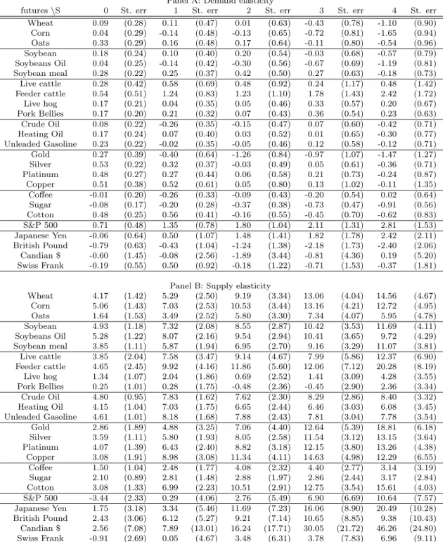
Demand and supply factors

The difference in the performance of the ultimate risk for our futures data relative to stock market data needs further analysis.15 As outlined in Breeden (1980) commodity betas may depend on their supply and demand elasticities and the covariances of goods’ production with aggregate consumption. For instance, a positive demand shock will for many commodities lead to higher prices, but will also be associated with higher

con-14_{The results for the contemporaneous case (S=0) differ slightly from the ones reported in Table 2.5,}

because the sample period for returns is shorter as we use future consumption growth.

15_{Note that our results appear to be robust with respect to the sample period, the sample size, the}

consumption measure, the use of real or nominal series (these auxiliary results are available from the authors on request).

(37)

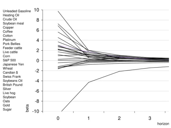
sumption, implying a positive short term beta. Following the demand shock however, demand may lower (because of a negative price elasticity) and supply may gradually increase, which both have off-setting effects on the relation between commodity prices on the one hand and longer term consumption on the other hand. Similarly, following a positive supply shock, prices will decrease and consumption will increase, leading to a negative short-term beta. Again, changes in demand and supply for the commodity following the price change will have off-setting effects in the longer run. Furthermore, French (1986) pointed out that demand and supply shocks to the current output are transmitted to future periods through inventories. The change in inventories is spread between consumption and storage, hence only part of the shock will affect future con-sumption.

Figure 2.3 provides some support for this, based on the consumption betas of our futures contracts. For each futures contract, the figure plots the beta with respect to the contemporaneous quarter consumption growth, as well as with respect to longer horizon consumpt