Generalized Spatial Regression with Differential Penalization
Matthieu Wilhelm
Director: Dr. Laura Maria Sangalli August 13, 2013
Master Project
Politenico di Milano
MOX, Laboratorio di Modellistica e di Calcolo Scientifico
Ecole polytechnique fédérale de Lausanne
Chaire de statistique mathématique, Prof. Victor M. PanaretosAvant-propos
Ce travail a été mené au cours d’un séjour au Politecnico di Milano, Italie, entre les mois de février et de juin 2013. J’ai été supervisé par le Dr. Laura M. Sangalli, chercheuse associée au laboratoire de modélisation et de calcul scientifique (MOX) du département de mathématique Francesco Brioschi du Politecnico di Milano. Ce projet s’inscrit dans le cadre de mon master en ingénierie mathématique entammé à l’Ecole polytechnique fédérale de Lausanne en septembre 2011.
Foreword
This work has been done during a stay at the Politecnico di Milano, Italy, between February and June 2013. I have been supervised by the Dr. Laura Sangalli, as-sociate professor at the modelling and scientific calculus laboratory (MOX) of the mathematical department “Francesco Brioschi” of the Politecnico di Milano. This thesis is a part of my master initiated in September 2011 at the Ecole polytechnique fédérale de Lausanne.
Résumé
Nous proposons une méthode noavatrice pour l’analyse de données spatialement dis-tribuées sur des surfaces dont les bords sont irréguliers et qui sont la réalisation d’une variable exponentielle. On considère le contexte des modèles additifs généralisés et l’on étend le travail de Sangalli et al. (2013) à des distributions autres que gaussiennes. En particulier, on peut alors considérer les distributions de famille exponentielle (par exem-ple des données binomiales, de Poisson ou de distribution gamma), et ainsi disposer d’un modèle avec un fort potentiel d’application. Pour l’ajustement du modèle, on maximise une fonction de log-vraisemblance pénalisée. Le terme de pénalisation tient compte d’un opérateur différentiel appliqué à la fonction que l’on cherche à estimer. Le modèle permet aussi d’inclure des informations auxiliaires telles que des variables explicatives. Le modèle proposé utilise des méthodes issues du domaine du calcul scientifique et fait en particulier usage de la méthode des éléments finis, qui permet d’imposer des conditions au bord à la fonction recherchée. Finalement, on étend de manière théorique le modèle développé pour des données distribuées sur une surface non planaire.
Abstract
We propose a novel method for the analysis of spatially distributed data from an expo-nential family distribution, able to efficiently treat data occurring over irregularly shaped domains. We consider a generalized linear framework and extend the work of Sangalli et al. (2013) to distributions other than the Gaussian. In particular, we can handle all distributions within the exponential family, including binomial, Poisson and Gamma out-comes, hence leading to a very broad applicability of the proposed model. We maximize a penalized log-likelihood function. The roughness penalty term involves a suitable differ-ential operator of the spatial field over the domain of interest. This maximization is done via a penalized iterative least square approach (see Wood (2006)). Covariate information can also be included in the model in a semi-parametric setting. The proposed models exploit advanced scientific computing techniques and specifically make use of the Finite Element Method, that provides a basis for piecewise polynomial surfaces and allows to im-pose boundary conditions on the space distribution of the probability. Finally, we extend theoretically the model to deal with data occurring on a two dimensional manifold.
Key words
Generalized additive models, spatial spline regression, finite element method, penalized regression
Thanks... I’m very grateful to Professor Victor Panaretos who gave me the chance to make a very interesting master thesis. I also would thank Dr. Kjell Konis who made me like computational statistics being my mentor with R.
Ringraziamenti... Vorrei ringraziare Laura M. Sangalli per avermi proposto un soggetto stimolante che ha rapresentato una degna fine del mio percorso di studi. Mi ha seguito con cura e attenzione durante questi mesi. Oltre all’aspetto scientifico, mi ha coinvolto nel gruppo di statistica del MOX e per questo gliene sono molto grato. Vorrei ringraziare Bree, per il suo aiuto nel risolvere certi problemi. La ringrazio soprattutto di avere condiviso con me tutte le pause gelato, momenti simpatici e allegri, sempre piacevoli a fine giornata. Vorrei ringraziare i miei colleghi del gruppo di statistica del MOX: la loro accoglienza e i pranzi del venerdì rimarranno dei bei ricordi.
In ultimo, vorrei ringraziare la comunità del Tender. Non ha prezzo arrivare la mattina in ufficio e sentire un atmosfera così cordiale e simpatica. In particolare, vorrei ringraziare Anna, Marianna, Ilaria, Franco, Mirko, Nur, Domenico, Anwar, Guido Abramo e Davide. Senza dubbio, è il migliore ufficio in cui sarò mai stato!
Remerciements... La fin des études est sans aucun doute, pour ceux qui ont la chance d’en faire, un rite de passage important. Cela marque le début de l’indépendance matérielle et donc la fin d’une époque, celle de l’éducation, de l’élévation (quand bien même ce terme demeure peu usité en ce sens). Je tiens donc à remercier mes parents, Luc et Luisa de m’avoir élevé, jusqu’à l’indépendance à laquelle je peux prétendre aujourd’hui. Ils m’ont donné
l’amour et la sécurité qui m’ont permis d’être ce que je suis aujourd’hui. Ils m’ont transmis les valeurs qui me permettent d’aborder avec confiance la vie qui s’offre à moi. Plus qu’un remerciement, c’est un hommage que je souhaite leur rendre en cette occasion.
Je ne serais pas non plus ce que je suis sans mes deux frères, Pierre et Lionel. L’âge adulte nous aura permis de fonder notre unité. Je ne serai jamais seul, et je leur dois cette
rassurante et intime conviction. Nous sommes le meilleur exemple que l’ensemble peut-être plus grand que la somme des parties.
Je ne peux pas évoquer ma famille proche sans évoquer Sophie, ma très chère belle-soeur. Si notre famille est si harmonieuse, c’est en partie grâce à elle.
Je souhaite rendre hommage à mes grands-parents et à mes nonni, François et Françoise Wilhelm, Angelo e Elisa Mozzi-Strick. Outre l’affection qu’ils nous ont toujours
généreusement témoignée, par leur vie et leur histoire, ils ont été et sont toujours pour nous de véritables exemples. Cette dernière année, passée entre août et décembre à Neuchâtel et à Milan entre février et juin m’a permis de partager de beaux moments avec eux. Je suis
conscient de la rare chance de pouvoir encore jouir de leur présence et je suis particulièrement heureux de pouvoir rentrer dans la vie active en les ayant encore à mes côtés. Mes
grands-parents et mes nonni représentent une génération qui a fait des sacrifices conséquents pour que les générations suivantes, c’est-à-dire nous, puissent vivre mieux. C’est l’occasion pour moi de leur témoigner ma gratitude car ces peines et ces sacrifices n’ont pas été vains. Je souhaite remercier mon parrain et ma marraine, Guy et Christiane Rambaud. Tout au long de ma vie, ils ont assumé avec conviction la charge qu’ils avaient accepté le jour de mon baptême. Ils sont et demeureront pour moi des références.
Je n’ai pas passé ces années à l’EPFL totalement seul. Mes compagnons d’études, mes compagnons de galère, m’ont été d’un grand soutient. Je veux les remercier pour tous les moments et toutes les discussions passées ensemble, pour tous les services qu’ils m’ont rendu et pour avoir rendu ces années agréable. Je veux en particulier remercier Reda Boumasmoud, Denis Devaud, Adrien Hitz et Thomas Lugrin. Je garderai un merveilleux souvenir de ma
volée, dans laquelle j’inclus abusivement Cyril, avec de beaux moments partagés, en
particulier à Istanbul lors de notre voyage d’étude, lors de la préparation de celui-ci et lors des différents séjours à Zinal.
Pour leur longue et indéfectible amitié, je tiens à remercier Matthieu, Raphaëlle, Marina. Ils sont pour moi l’incarnation de ce que devrait être l’amitié: de la loyauté, de la chaleur, du respect et des bons moments à revendre!
Finalement, ma vie ne serait pas la même sans Marie à mes côtés. Elle sait combien cela me rend heureux.
Fais confiance au Seigneur, agis bien, habite la terre et reste fidèle, Psaumes (36.3)1
Contents
1 Introduction 11
2 Model and Motivation 13
2.1 Data and model . . . 13
2.2 The framework: the exponential family . . . 14
2.3 Penalized iterative reweighted least squares algorithm . . . 15
2.4 Weighted penalized least square minimization problem . . . 16
3 Finite Elements Formulation 19 3.1 A very short introduction . . . 19
3.2 Reformulation of the problem . . . 19
3.3 From weak formulation to linear systems . . . 20
3.4 Explicit form of the estimates . . . 22
3.5 Generalization to a mesh independent of the data points . . . 22
4 Justification of the PIRLS algorithm and penalized log-likelihood 25 4.1 Functional derivation of the PIRLS algorithm . . . 25
4.2 Derivation of the penality matrix . . . 28
4.3 Finite dimensional derivation of the PIRLS algorithm . . . 29
5 Smoothing parameter choice and variance estimation 31 5.1 Choosing the smoothing parameter: a bias/variance trade-off . . . 31
5.2 Choosing the smooth parameter: the generalized cross validation . . . 32
5.3 Variance and scale parameter estimation . . . 33
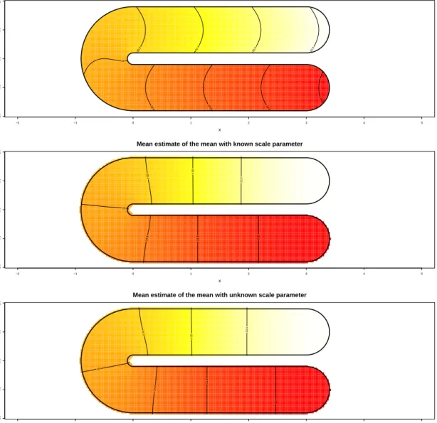
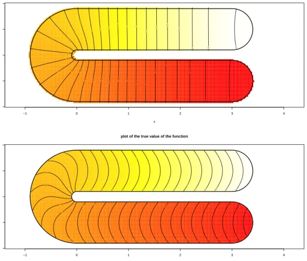
6 Simulations 35 6.1 Meshes and data . . . 36
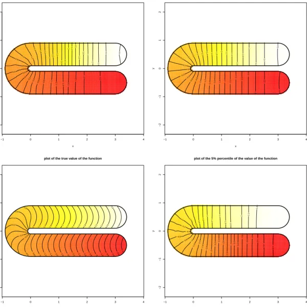
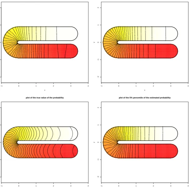
6.2 Simulations without covariates . . . 38
6.2.1 Binary responses . . . 38
6.2.2 Gamma responses . . . 44
6.3 Simulations with covariates . . . 46
6.3.1 Binary responses with covariates . . . 46
6.3.2 Gamma responses with covariates . . . 46
6.4 Confidence intervals and distributional results . . . 53
6.5 Comparison with other methods . . . 55
8 A first approach to non planar domains 61 8.1 A geometric framework . . . 62 8.2 Finite element solution in the case of surface embedded in R3 . . . 63
9 Conclusion and perspective 65
Notations
For a vector, bold lower case is used, for example µ. When a similar symbol in normal font and with an index i is used, e.g µi, it denotes the ith component of the vector µ. Bold upper
case is used to denote a matrix. For example X denotes the design matrix. Normal lower case usually denotes functions. Maximum likelihood, or maximum penalized likelihood estimates are denoted with a hat, e.g., ˆβ. When a single variable function is applied to vector, it results in vector whose components are the evaluation of the function at the components. For example,
Chapter 1
Introduction
Many datasets are considered as realizations of functions disturbed by random noise. These data, called functional data, suggest that we seek to estimate the underlying function that generated such a process. This type of analysis is relatively recent and is a very active field of research in statistics (Ramsay and Silverman, 2005).
In this context, we aim to estimate a function. This unusual since we generally aims to estimate parameters lying in a finite dimensional space. In the case of an estimation of a function, the estimation process is generally in two stages. First, a subspace of finite dimension of the functional space in which the functionf (or is assumed to lie) the true function is chosen. Then, the problem of estimating becomes a parametric estimation. The choice of this finite dimensional subspace is then crucial and is usually subjective. As examples of finite dimensional spaces, we can mention the subspace spanned by the Fourier basis, usually used for periodic functions, or the subspace spanned by polynomials of a finite degree.
This project aims to extend the methodology developed in Sangalli et al. (2013). The finite dimensional space used is generated by the finite element method. The finite element method is widely used in the field of numerical approximation of partial differential equations (PDE’s). It allows to make approximations which are piecewise polynomial surfaces. In addition, they are suitable for estimates over complex domains, which is common in the field of PDE’s, and allow to take into account boundary conditions. These characteristics make them particularly suited to the context of functional data analysis (for an introduction to finite elements, see Quarteroni (2009)).
The model developed in Sangalli et al. (2013) uses a least square error formulation which can be also viewed as the log-likelihood of normally distributed data to approximate spatial functions. This is not well suited for spatial distributed binary data, for example. The pur-pose of this project is to extend this model to other distributions such as Bernoulli, Poisson or Gamma. We use a methodology inspired from the one used to extend linear models to generalized linear models. In addition, as it is commonly done in the area of functional data analysis, a penalty ensures that the estimated function is smooth enough.
Chapter 2
Model and Motivation
In this project, our aim is to extend the model developed in Sangalli et al. (2013) to other distributions than normal distribution. We propose a generalized additive model (GAM), also called as generalized semiparametric regression model, (see Hastie and Tibshirani (1986, 1990); Wood (2006); Bickel et al. (1993)).
Let{pi = (p1i, p2i);i= 1, . . . , n} be a set ofn points on a bounded regular domain Ω⊂R2,
zi the corresponding value of the observed variable at the point pi and let xi = (x1i, . . . , xqi)t
be aq-vector of covariates associated to the observationyi. The goal is to deal with models of
the type:
g(E[Yi |xi,pi]) =xitβ+f(pi), Yi |xi,pi ∼exponential family distribution (2.1)
where g(.) is a link function (see section 2.2 for details about exponential family distribution). We aim to estimate both β∈Rq and f ∈ F, a function which belongs to a functional space F
to be defined. Many different methods have been developed to deal with this kind of problems. Since the function f belongs to a functional space, it is usual to estimate the function f using FK, a finite dimensional approximation of the (hilbertian) functional spaceF of dimensionK ∈
N. Using a basis {ψ1, . . . , ψK} of FK, the problem (2.1) simplifies to a traditional generalized
linear model (GLM).
The goal of this project is to find an efficient way to compute estimates of the vector β and of the function f. As for a traditional GLM, we will use an iterative algorithm to approximate the solution of the maximum likelihood, called Iterative Reweighted Least Squares (IRLS, see McCullagh and Nelder (1989, p. 40-43)). In this case, we will use particular case of this algorithm to take into account the penalization of the functions that must ensure a sufficient smoothness of the approximation of the function f.
2.1
Data and model
We wish to estimate the parameter β and the function f, according to model (2.1).
A roughness penalization of the function f is needed in order to avoid overfitting of the function. The iterative procedure aims to compute, for a given value of λ, the maximum likelihood estimates ˆβ ∈Rq and ˆf ∈ F
K of the model, corresponding to the maximum of the
penalized log-likelihood function: Lp(β, f) = n X i=1 l(yi;ηi(β, f))−λ Z Ω (∆f)2, (2.2)
where, l(·) is the log-likelihood, ηi = xitβ +f(pi) and λ is a positive constant. In the case
of the quadratic form of the penalized log-likelihood function. Actually, this functional can be written as: LGaussian(β, f) =ky−Xβ−fnk2−λ Z Ω (∆f)2,
where fn = (f(p1), . . . , f(pn))t. In the Gaussian case, the optimum is simply the solution
of a linear system which is obtained after discretization of the functional space F (Sangalli et al., 2013). In the more general case of a distribution belonging to the exponential family, the penalized log-likelihood function may not be a quadratic form. We use an iterative algorithm to find this optimum. One of the well-known methods used in the context of GLM is the Iterative Reweighted Least Square (IRLS, (McCullagh and Nelder, 1989)). The idea is to compute at each step a weighted least square estimation. In our case, due to the penalization term, we will use a slightly different form of this algorithm, called Penalized Iterative Reweighted Least Squares (PIRLS, see Wood (2006) or Wood (2011)). This allows us to use the procedure developed in Sangalli et al. (2013) at each step of the algorithm.
2.2
The framework: the exponential family
A random variableY is said to belong to the exponential family if its distribution can be written as:
fY(y) = exp{(yθ−b(θ))/a(φ) +c(φ, y)},
wherea(·),b(·) andc(·) are arbitrary functions subject to some regularity constraints (McCul-lagh and Nelder, 1989). The parameter θ is called canonical parameter and φ is called scale parameter. In the context of GLM, we have g(µ) = η, where µis the mean, g(·) a link function and η = xtβ is called the natural parameter. So η is modelled as a linear combination of the
observation x and thus, influence the modelling of the distribution. Link functions are con-tinuous, strictly monotonic functions and are therefore invertible. On one hand, we have the following properties, for general maximum likelihood estimates:
E0 " ∂l ∂θ θ=θ 0 # = 0, var ∂l ∂θ θ=θ 0 ! = E0 " ∂l ∂θ 2 θ=θ0 # , E " ∂l ∂θ 2 θ=θ0 # = E0 " ∂2l ∂θ2 θ=θ 0 # , (2.3)
where θ0 is the maximum likelihood estimate and the subscript 0 is to emphasize that the
expectation is taken with respect to the density function f(y;θ0). On the other hand, simple
calculations show that, for an exponential family distribution, we have:
E " ∂l ∂θ !# = E[Y]−b 0(θ) a(φ) . Thus, we have: b0(θ) = µ.
Using the second and the third property of (2.3), we have then: var(Y) =b00(θ)a(φ).
Until now, we have made no restrictions about the functiona(·). Actually, it is usual to consider distribution where a(φ) is of the form a(φ) = φ/r, which allows heteroscedastic models and
covers all the cases of practical interest (Wood, 2011, p.63). More complex forms of a(·) won’t be considered here. Usually r is set to 1. Thus in this case the variance can be written as:
var(Y) = b 00(θ)φ
r .
Since θ depends on the mean µ, we can always define a function V(·) such that var(Y) =V(µ)φ.
This function is called variance function. Under regularity conditions, and since we haveb0(θ) =
µ, we have:
V(µ) =b00((b0)−1(µ)),
where, (b0)−1(·) is the reciprocal function of the first derivative with respect toθof the function
b(·).
On one hand we have b0(θ) = µ and the other hand, we have g(µ) = η =xtβ. In the case
where η = θ, that is b0(·) = g−1(·), the link function is said to be canonical. Therefore, for every exponential distribution, there is a canonical link function. For the binomial distribution, the canonical link function is the logit function. Other link functions are available for binary responses such as the probit or the c-loglog. The choice of the link function is not discussed since it is not the purpose of this work.
2.3
Penalized iterative reweighted least squares algorithm
The goal of this algorithm is to approximate the optimum of the functional given in (2.2). To achieve this, we approximate at each step of the algorithm the penalized negative log-likelihood (up to a scale factor) with a quadratic form and we solve a simpler least square problem. The main problem is that the penalized log-likelihood optimisation problem is complex to solve since the link function g is usually not linear (except in the Gaussian case) and therefore, we use this iterative procedure. Let λ be a positive smoothing parameter. For a given vector µj, we define: ηj =g(µj), X= xt 1 .. . xt n , Wj = diag 1 V(µj)(g0(µj))2 ! ,fn= (f(p1), . . . , f(pn))t,
where V(·) is the variance function associated to the distribution of the observations, and g is the link function1. We can then approximate the solution of minimizing (2.2) as the minimum of (see section 4 for a rigorous justification):
˜
Jλ(β, f) = k(Wj)1/2(zj−Xβ−fn)k2+λ Z
Ω
(∆f)2,
where zj = ηj +g0(µj)(y−µj) is called “pseudo-data”, i.e., the first order approximation of
g(y), assuming that yis in the neighbourhood ofµj.
Given µj, the algorithm is the following: 1. Computeηj, zj and Wj.
2. Solve the problem of finding ˜βj and ˜fj that minimize k(Wj)1/2(zj −Xβ−fn)k2+λ
Z
Ω
(∆f)2 (or a finite dimensional approximation of this functional)
3. Setµj+1 =g−1(Xβ˜j+ ˜fj
n)
For the initialization, we set µ0 =yexcept in the logistic case where µ0 = 1/2(y+ 1/2).
There are various convergence criteria to detect convergence of the process, here we use one based on a sufficiently small variation of the objective function between two iterations.
Such an iterative process is usual in the context of GAM and the particularity of our method is in finding an efficient way to solve the minimization problem at the step 2 of the algorithm.
2.4
Weighted penalized least square minimization
prob-lem
Given the current (diagonal) weight matrix W and a design matrix X, we want to minimize the following functional with respect to (β, f):
˜
Jλ(β, f) =kW1/2(z−Xβ−fn)k2+λ Z
Ω
(∆f)2. (2.4)
We will add a tilde over variables which achieve the minimum of the functional ˜Jλ. First, we
need to recall a classical result known as the Lax-Milgram lemma, which will be used later: Proposition 1
Let F be a Hilbert space, G(·,·) : F × F → R a continuous and coercive bilinear form,
F(·) : F → R a linear and continuous functional. Then there exists a unique solution to the problem:
find u∈ F such that: G(u, v) =F(v), ∀v ∈ F.
Moreover, ifG(·,·) is symmetric, thenucharacterize the unique minimizer inFof the functional
J(·) :F →R, defined as
J(v) =G(v, v)−2F(v).
The Lax-Milgram lemma states an equivalence between two problems. We will use this fact to solve a equivalent problem instead of minimizing (2.4). Now we can show the following result:
Proposition 2
IfX is a full-rank matrix, and ifWii6= 0, i= 1, . . . , n, the solution ( ˜β,f˜) to the minimization
problem (2.4) satisfies: 1. ˜β= (XtW X)−1XtW(z−˜f n), 2. ˜f satisfies: utnQ ˜fn+λ Z Ω (∆u)(∆ ˜f) =utnQ z, ∀u∈ F.
where Q = (I−H)tW(I−H) and H = X(XtWX)−1XtW. Moreover, the solution β˜,f˜
Proof. First of all, given f, the unique minimizer of the functional ˜Jλ(β, f) is given by:
˜
β(f) = (XtWX)−1XtW(z−fn). (2.5)
To show that, we take the derivative of ˜Jλ(β, f) with respect to β:
∂J˜λ(β, f)
∂β =−2X
tW(z−f
n) + (XtWX)β.
Since X is assumed to be a full-rank matrix and since W is invertible (Wii is assumed to be
strictly positive, because Wii 6= 0 andWii ≥0 by construction),XtWX is invertible. Finally
the necessary condition ∂J˜λ( ˜β, f)/∂β = 0 is satisfied if and only if ˜β is given by (2.5). Since
for fixed f, ˜Jλ(β, f) is clearly convex, ˜β is a minimum. For vector and matrices derivation
rules, see for example Felippa (2012).
SettingH=X(XtWX)−1XtW,Q= (I−H)tW(I−H), and plugging ˜β into the objective
function, we have the following form of the functional: ˜ Jλ(f) = ztQ z−2fnQ z+f t nQ fn+λ Z Ω (∆f)2. (2.6)
Since we want to optimize this functional with respect to the function f only, we can rewrite the problem (2.6) as:
find ˜f ∈ F that minimizes: Jλ(f) =f t
nQ fn+λ
Z
Ω
(∆f)2−2fnQ z, (2.7)
which could be written as G(f , f)−2F(f), where G is a symmetric, coercive and continuous, bilinear form onF × F and F a linear and continuous functional onF. Using the Lax-Milgram lemma and thanks to the symmetry ofG(·,·), the problem (2.7) is equivalent to the problem of
find ˜f ∈ F such that: G( ˜f , u) = F(u) ∀u∈ F.
The hypotheses of the Lax-Milgram lemma are fulfilled since the bilinear formGis coercive and continuous and since the linear formF is also continuous. The verification of these hypotheses are very simple and we do not address this issue. A rigorous proof of the equivalence of the problems and of the uniqueness of ˜f, applied to this particular case can also be found in Azzimonti (2013). In our case, we can identify the bilinear form Gas:
G(v, u) = utnQ vn+λ Z
Ω
(∆u)(∆v),
where un= (u(p1), . . . , u(pn))t, and the linear functional F as:
F(v) = vtnQ z.
So finally the solution of minimizing (2.7) is given by: find ˜f ∈ F such that: utnQ˜fn+λ
Z
Ω
(∆u)(∆ ˜f) =utnQ z ∀u∈ F. (2.8) The uniqueness of the minimizer is also stated by the Lax-Milgram lemma. We conclude that
˜
Chapter 3
Finite Elements Formulation
3.1
A very short introduction
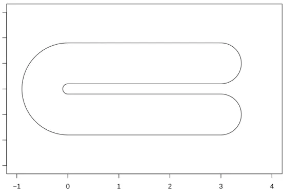
The Finite Elements Method (FEM) is a widely used method to compute numerical solutions of physical problems driven by partial differential equations. The idea is to find the best approximation belonging to a given finite dimensional space. First of all, we divide the domain, embedded inR2, into triangular subdomains. The set of triangles resulting from this process is called a mesh. The mesh generation is a very complicated procedure and a abundant literature is dedicated to this subject (see, for example Cheng et al. (2013)). Then we impose that finite element solution must be polynomial in x and y (in this case, polynomial of order 1 or 2) over all triangles and continuous across edges and vertices. For every node ξj, we define a function ψj which is piecewise polynomial of the prescribed order and such that we have
ψi(ξj) =δij, ∀j = 1, . . . , K. The dimension of the finite element space is then the number of
nodes, that is K. This kind of basis is referred to as Lagrangian finite elements. We will use a finite element basis to get a finite dimensional approximation FK of the functional space F.
Then, we will compute the “best” approximation ˆf ∈ FK of the function f. The meaning of
the word “best” is the following: since we are looking for the solution of the problem (2.7) and that G(u, v) is bilinear, symmetric and positive definite overF × F, it can be proven that the error is orthogonal to the solution in the sense of the inner product G(., .), that is the finite element solution is the projection of the true solution on FK. This property is called Galerkin
orthogonality.
For more informations about FEM, see for example Quarteroni (2009).
3.2
Reformulation of the problem
We have seen that we have to solve at each step of the PIRLS algorithm a minimisation problem. It has been shown that such a problem can be reduced to solving a linear system (Sangalli et al., 2013). We describe this procedure in the following discussion.
First of all, we recall the minimization problem to be solved at each step of the algorithm: min (β,f)∈Rq×F ˜ Jλ(β, f) =kW1/2(z−Xβ−fn)k2 +λ Z Ω (∆f)2,
where W is the diagonal weight matrix and z is the pseudo-data at the current step of the algorithm. The functional ˜Jλ(β(f), f) can be expressed as G(f, f)− 2F(f), as previously
stated (see equation 2.7). The minimization problem is then equivalent to solve the problem
G(f, u) = F(u), ∀u∈ F. This equivalent problem is calledweak formulation. We will describe the computations yielding to the solution of this problem.
First of all, given a function f, the maximizer of Jλ(β, f) is given by
˜
β= (XtW X)−1XtW(z−fn).
Moreover, ˜f must satisfy (2.7).
Now, we can recall a simple property of real hilbertian vector spaces. Let a,b∈ V, where
V is a real hilbertian vector space. We have the following property:
a=b⇔ ha,ci=hb,ci, ∀c∈V. (3.1) Therefore, we can characterize any vector of F since F is a real vector space. Thanks to this characterization, we will reformulate the problem (2.8) substituting ∆ ˜f by another function ˜g. Problem (2.8) then becomes:
utnQ˜fn+λ Z Ω (∆u)˜g =utnQ z, ∀u∈ F, Z Ω (∆ ˜f) v = Z Ω ˜ g v, ∀v ∈ F. (3.2)
This justification is only formal since the functional spaces used are Sobolev spaces. Actually all the functions considered are defined up to a set of null measure. We only want to give an intuition to the reader. For a more rigorous development, see Azzimonti (2013, chapter 2).
From the Green formula we get:
Z Ω (∆u)˜g =− Z Ω ∇u· ∇g˜+ Z ∂Ω ˜ g∂u ∂n,
wheren denotes the outward-pointing normal vector to the boundary. In our case, we consider functions whose normal derivative vanishes on the boundary, hence we have
Z ∂Ω ˜ g∂u ∂n = 0. We get then: utnQ ˜fn−λ Z Ω ∇u· ∇g˜=utnQ z ∀u∈ F, − Z Ω ∇f˜· ∇v = Z Ω ˜ g v ∀v ∈ F. (3.3)
In this setting, we will find two different functions, ˜f and ˜g. In a finite dimensional space, (3.3) results in a sparse linear problem.
These computations, apparently easy, are only formal. To justify this development, strong and subtle hypotheses are required. Such a rigorous approach is done in Azzimonti (2013).
3.3
From weak formulation to linear systems
We will show how the weak formulation problem leads to a linear problem using finite elements. Let ˆF be a K dimensional finite element subspace of F. Then both equations of the problem (3.3) could be written in the form:
˜
G(h, u) = ˜F(u) ∀u˜∈ FK, (3.4)
where ˜Gis a symmetric, bilinear form and ˜F is linear functional. SinceFK is finite dimensional,
of the basis, thanks to the bilinearity of ˜Gand to the linearity of ˜F, then it will be satisfied for any element of FK. We can expand any function h∈ FK in the basis of FK as:
h(x) =
K X i=1
hiψi(x), hi ∈R, ∀i= 1, . . . , K,
which can also be written as: ˜
h=htψ, where h= (h1, . . . , hK)t, and Ψ= (ψ1(x), . . . , ψK(x)).
Finally, we get the following linear system:
K X i=1
hi G˜(ψi, ψj) = ˜F(ψj), ∀j = 1, . . . , K.
Using this, we only have to compute the values ˜G(ψi, ψj) and ˜F(ψj), i, j = 1, . . . , K and solve
the system.
In our case, for the first equation, we have:
G1(s, t) = stnQ tn−λ Z
Ω
∇s· ∇t, F1(s) =stnQ z.
and for the second one:
G2(s, t) = Z Ω ∇s· ∇t+ Z Ω s t, F2(s) = 0.
Instead of Ω, we will use ΩT, a polygonal approximation of the domain, resulting in a regular triangulation of Ω.
Finally, this allows us to construct the linear system. We define the K ×K matrices R0
and R1, called mass and stiffness matrix respectively, as:
(R0)ij = Z ΩT ψi ψj, (R1)ij = Z ΩT ∇ψi· ∇ψj.
We introduce the order K block matrixL and the K×n block matrixP1, defined as:
L= Q On×(K−n) O(K−n)×n O(K−n)×(K−n) and P1 = In O(K−n)×n .
Finally, if ˜f and ˜g denote the vectors of coefficients of the expansion of the functions ˜f and ˜g
in the basis ψ, we can write the linear system corresponding to the problem (3.4) as:
" −L λR1 λR1 λR0 # " ˜ f ˜ g # = " −LP1z 0 # . (3.5)
For computational reasons, we have symmetrised the problem. In this context, ˜g = ˜gtψ is an
approximation of the function ∆ ˜f. In order to get the vector ˜fnwhich is the vector of the values
of ˜f evaluated at the points p1, . . . ,pn, we need the values of the coefficients of the vector ˜f
corresponding to these points. We choose a triangulation such that the vertices of the triangles coincide with the locations of the observation. Hence thanks to the fact that, for a given node
ξi, we have ψj(ξi) =δij, where δij is the Kronecker symbol, we have ˜f(pi) = ˜fi. We can then
estimate the value of the functional that we have minimized at the current estimates as: ˜ Jλ( ˜β,˜f,g˜) = z−Xβ˜−˜fn t Q z−Xβ˜−˜f+λ g˜t R1 ˜g
3.4
Explicit form of the estimates
Thanks to (3.5), we can give the explicit forms of the estimates: ˜
f =L+λR1R−01R1
−1
LP1z.
Since we have chosen a mesh whose internal nodes coincide with the data, writing, P2 =
[In On×K−n], we have: ˜ fn=P2˜f =P2 L+λR1R0−1R1 −1 LP1z.
Replacing that value in (2.5), we get: ˜ β = (XtWX)−1XtW(z−˜fn) = (XtWX)−1XtW−P2 L+λR1R0−1R1 −1 LP1 z.
We can then conclude that both estimates, ˜β and ˜f depend linearly on the pseudo-data z. However, since the pseudo-data do not depend linearly of the data themselves, we cannot use this fact to give closed expressions for the mean and for the variance, as it is done in Sangalli et al. (2013).
We can finally define the hat matrix R for the generalized additive model (see Hastie and Tibshirani (1990, p. 156)) as the matrix such that, at convergence:
ˆ
η =Rz, (3.6)
where ˆη is the natural parameter at the convergence andz is, in this context, the last pseudo-data, i.e., the pseudo data at the convergence. In this case, the hat matrix is given by:
R= (XtWX)−1XtW+ (I−X)P2 L+λR1R−01R1 −1 LP1 .
This hat matrix is important because it is the matrix which define the equivalent degree of freedom. See section 5.2 for more details.
3.5
Generalization to a mesh independent of the data
points
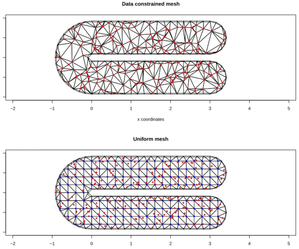
We saw that it might be convenient to use a mesh whose internal nodes are exactly the location of the data points. Obviously, it is useless to refine the mesh where there is no data points and at the contrary, it seems reasonable to have a finer mesh where there is higher density of data points. In this case the finite element subspace becomes then dependent of the location points. If we use a constrained mesh where the internal nodes coincide with the location of the data, setting that fori= 1, . . . , n, ψi is the basis function corresponding to the location pi, the
unknown ˜fn, defined as:
˜f
n= ( ˜f(p1), . . . ,f˜(pn))t,
is also the n first components of the unknown vector ˜f. We can then easily solve the system (3.5).
On the contrary, if the location points do not coincide with nodes, we do not have the fact that ˜fi = ˜f(pi),∀i = 1, . . . , n. So we have to compute the value of fn related to the vector ˜f.
LetΨ be the n×K matrix defined as:
Then ˜fn=Ψ˜f. The system becomes (3.5): " −Ψt Q Ψ λR1 λR1 λR0 # " ˜ f ˜ g # = " −ΨtQ z 0 # . (3.7)
Indeed, the penalization matrix is not influenced by this modification and the other blocks of the matrix (3.7) are identical to those of (3.5).
The computation of the estimates then becomes: ˜f = Ψt Q Ψ+λR1R−01R1 −1 ΨtQz, and ˜ β = (XtWX)−1XtW(z−˜fn) = (XtWX)−1XtW−ΨΨt Q Ψ+λR1R−01R1 −1 ΨtQ z.
As in the case of data constrained mesh, we can easily define a matrix R such that ˆη = Rz, where z is the pseudo-data at convergence.
Chapter 4
Justification of the PIRLS algorithm
and penalized log-likelihood
Since our model can be seen as a generalized additive model, we will use methods developed in this context (Hastie and Tibshirani, 1986, 1990; Wood, 2006). In particular, the PIRLS algorithm is suitable for our model. PIRLS aims to compute the maximum penalized likelihood estimates β ∈Rq and ˆf ∈ F
K. Let m(., .) be a bilinear, symmetric and positive definite form
on F × F that represents the penalization. In our case, we are seeking to find the maximizer of the following penalized log-likelihood:
Lp(β, f) = L(β, f)−λ m(f, f), (4.1)
where, L(β, f) is the log-likelihood of the model. Until now, we do not have made precise assumptions about the functional space F in which lies the functionf. A necessary condition to ensure the existence of a solution to the problem of minimizing (4.1) is that f ∈ H2(Ω).
Moreover, suitable boundary conditions are required to ensure well-posedness of the problem. For more precise references about the functional framework, we refer to Azzimonti (2013). In particular, the use of a mixed finite elements approach for a 4 order minimization problem is discussed.
The problem of maximizing the penalized log-likelihood is non-trivial since we deal with functional spaces. As already mentioned, solving this problem is a two step process. The two steps are the discretization and the optimization. If we first discretize and then optimize, we seek an optimum in a finite dimensional space, which is a well-known problem. We can also first optimize in the functional space and then find a finite dimensional approximation of this optimum. These approaches are well-known in the context of optimal control theory. In this work, we develop both approaches. Obviously, the so-called optimize-discretize approach is more complex since the optimization is done in a functional space. In our case, this allows us to reformulate the problem in order to use a similar approach to the one used in Sangalli et al. (2013). Without that, we would not have obtained the problem of minimizing (2.4).
4.1
Functional derivation of the PIRLS algorithm
We know that the maximum values ( ˆβ,fˆ) of the functional (4.1) satisfy the following equations:
∂L( ˆβ,fˆ) ∂βj = 0, ∀j = 1, . . . , q, lim t→0 1 t h L( ˆβ,fˆ+tu)− L( ˆβ,fˆ)i−λ m(u,fˆ) = 0 ∀u∈ F. (4.2)
Actually, since ˆf ∈ F, andF is infinite dimensional, we would have to consider the maximiza-tion problem in an infinite dimensional space. We aim to compute the Gâteaux derivative of the penalized log-likelihood to get the variational formulation of the minimization problem seen in (2.4). The Gâteaux derivative is defined for functions in locally convex topological vector spaces, such as Banach spaces and is a generalization of the concept of directional derivative. Actually, the functional spaces used in our context are Sobolev spaces. The log-likelihood func-tion L depends on β and f because the natural parameterθ depends on β and f. Given any function u∈ F, and any real number t, we then have:
L(β, f +tu)− L(β, f) = = n X i=1 ri φ [(yiθi(β, f +tu)−b(θi(β, f +tu))−yiθi(β, f) +b(θi(β, f)))] = n X i=1 ri φ(yiθi(β, f+tu)−yiθi(β, f)−(b(θi(β, f+tu))−b(θi(β, f))).
Dividing this expression by tand taking the limit as t tends to 0 gives the Gâteaux derivative. We have then: ∂L(β, u) ∂f = limt→0 1 t [L(β, f+tu)− L(β, f)] = lim t→0 1 t n X i=1 ri φ [yiθi(β, f+tu)−yiθi(β, f)−(b(θi(β, f+tu))−b(θi(β, f))] ! = n X i=1 ri φ " yi ∂θi(β, u) ∂f −b 0 (θi(β, f)) ∂θi(β, u) ∂f # .
where b0(·) stands for ∂b∂θ. We have then to compute the value of ∂θi(β, u)
∂f . Recalling that we
have E[Yi] =µi =b0(θi) and taking the derivative, we get:
∂µ ∂θ =b 00 (θ)⇒ ∂θ ∂µ = 1 b00(θ) and hence: ∂θi(β, u) ∂f = 1 b00(θ i) ∂µi(β, u) ∂f .
We can conclude that we have:
∂L(β, u) ∂f = 0 ⇔ n X i=1 ri φ (yi−b0(θi)) b00(µ i) ∂µi(β, u) ∂f = n X i=1 (yi−b0(θi)) var(Yi) ∂µi(β, u) ∂f = 0.
Since we have var(Yi) = V(µi)φ and b0(θi) = µi, we have:
∂L(β, u) ∂f = 0⇔ n X i=1 (yi−µi) V(µi) ∂µi(β, u) ∂f = 0.
On the other hand, we have to compute the derivative of the functional Lp with respect to
β. Hence we have: ∂Lp(β) ∂βj = n X i=1 ri φ yi ∂θi ∂βj −b0(θi) ∂θi ∂βj ! . Since we have ∂θi ∂βj = ∂θi ∂µi ∂µi ∂βj = 1 b00(θ i) ∂µi ∂βj ,
We finally get: ∂L(β) ∂βj = 0 ⇔ n X i=1 (yi−µi) V(µi) ∂µi ∂βj = 0.
Putting all these results together and assuming that V(µi) is fixed, the solution of (4.2) is
equivalent to findingµ that satisfies
n X i=1 (yi−µi) V(µi) ∂µi ∂βj = 0, ∀j = 1, . . . , q, n X i=1 (yi−µi) V(µi) ∂µi(β, u) ∂f +λ m(f, u) = 0 ∀u∈ F,
which is itself equivalent to find the solution of minimizing the functional S: S =kV−1/2(y−µ)k2+ λ
2 m(f, f),
whereV= diag(V(µ1), . . . , V(µn)), but considering this fixed and hence suggesting an iterative
computation.
We then develop a first order approximation of µin the neighbourhood of the current value (β0, f0). We have: µ(β,f) = g−1(Xβ0+fn0) | {z } =µ0 +∂µ(β, f) ∂β (β−β 0 ) + ∂µ(β, f) ∂f .
We have the to compute the partial derivatives of µ with respect to both variables β and f. Since we have g(µ0i) =xtiβ0+ [fn0]i ⇒ ∂ ∂βj g(µ0i) = g0(µ0i)∂µ 0 i ∂βj = ∂ ∂βj xtiβ0 =Xij ⇒Jij = Xij g0(µ0 i) , we get then: µ(β, f) ∂β = (G 0)−1X,
where G0 = diag(g0(µ0)) and X is the design matrix.
Since µ(β, f) = g−1(η(β, f), η = (Xβ+f
n), for the Gâteaux derivative of µ(β, f), in the
direction f, we have for ith component: lim t→0 µi(β0, f0+tf)−µi(β0, f0) t = lim t→0 g−1(η i(β0, f0+tf))−g−1(ηi(β0, f0)) ηi(β0, f0+tf)−ηi(β0, f0) ηi(β0, f0+tf)−ηi(β0, f0) t = 1 g0(µ0 i) [fn]i,
and thus we finally have a first order approximation of S in the neighbourhood of the current value (β0, f0):
S ≈ kV−1/2(G0)−1(G0(y−µ0)−η0−fn)k2 +
λ
where η0 = Xβ0. Setting z0 = η0 +G0(y−µ
0), and W0 the diagonal matrix such that
(W0)
ii=
1
V(µ0
i)g0(µ0i)2
, we can write S as:
S ≈ k(W0)1/2(z−Xβ−fn)k2 +
λ
2 m(f, f).
Since W0 is positive definite, S is approximately a quadratic form whose minimum exists and
is unique.
The likelihood of an exponential family distribution is strictly concave if a canonical pa-rameter is used. Since the penalization term is concave too (it is minus a positive term), the maximum of the penalized log-likelihood is unique, when it exists. Therefore, if the convergence of the PIRLS is reached, it always results in the maximum penalized log-likelihood estimate.
4.2
Derivation of the penality matrix
If we consider the problem of minimizing the functional (4.1), it leads to an infinite dimensional minimization problem. To avoid this problem, we discretize the penalization operator, in our case the integral of the square of the Laplacian.
We consider any function h ∈ FK, where FK is K-dimensional finite element space with
basis functions {ψ1(x), . . . , ψK(x)}. We consider ΩT, a triangulation of the domain Ω. Our penalization of the function is then written as:
p(h) = Z ΩT (∆h)2 = Z ΩT ∆h ∆h.
Setting g = ∆h we can write:
p(h) =
Z
ΩT
∆h g, such thatg = ∆h.
Using the characterization of (3.1), we can write:
p(h) = Z ΩT ∆h g, such that Z ΩT g v = Z ΩT ∆h v ∀v ∈ FK.
Using the Green formula and thanks to the homogeneous Neumann boundary conditions, we obtain: p(h) = − Z ΩT ∇h· ∇g such that Z ΩT g v =− Z ΩT ∇f · ∇v ∀v ∈ FK. Since R ΩT g v =− R
ΩT ∇h· ∇v must be satisfied for all v ∈ FK, it is sufficient to satisfies this condition for any element of the basis. We define the K×K matrices R0 and R1 as in section
(3.3). Writing h and g as htψ and gtψ, we get:
p(h) =−htR1 g such thatR1 h+R0 g = 0.
Finally, we can write the penalization of the function h as:
p(h) =ht R1t R−01R1 h.
We can conclude that the penalization matrix can be written as: ˜
4.3
Finite dimensional derivation of the PIRLS
algo-rithm
We are looking for the minimum of the penalized log-likelihood function. Let be β∗ = (β,f)t,
where β ∈ Rq and ft is the vector containing the values of coefficients defining the function
ˆ
f ∈ FK. For sake of simplicity letN =q+K be the dimension of the vectorβ∗. We can write
the finite dimensional approximation of the penalized log-likelihood as:
lp(β∗) =l(β∗)−λ β∗ t
S β∗,
where S is a N ×N penalization matrix defined as: S = Oq×q Oq×K OK×q ˜S .
Since we consider realizations of an exponential family distribution, we can write the density of yi, with natural parameter θi, which depends of β∗, and scale parameter φ, as:
fθi(yi) = exp{(yiθi−b(θi))/ai(φ) +c(φ, yi)}.
The functions b(·) and c(·), are arbitrary defined and we set that a has the form ai(φ) = rφi
and, in this case ri = 1. This choice is explained in the section 2.2. The log-likelihood of the
model is then: l(β∗) = n X i=1 ri[(yiθi−b(θi))/φ+c(φ, yi)].
Hence, the derivative of l(β∗) with respect to β∗j is:
∂l(β∗) ∂βj∗ = 1 φ n X i=1 ri yi ∂θi ∂βj∗ −b 0 (θi) ∂θi ∂βj∗ ! .
Using the chain rule, we have:
∂θi ∂βj∗ = ∂θi ∂µi ∂µi ∂βj∗.
Since we have µi =b0(θi), for any distribution belonging to the exponential family, we have:
∂µi ∂θi =b00(θi)⇒ ∂θi ∂µi = 1 b00(θ i) . We have then: ∂l(β∗) ∂βj∗ = 1 φ n X i=1 (yi−b0(θi)) b00(θ i)/ri ∂µi ∂βj .
Since we have var(yi) =b00(θi)φ=V(µi)φ, we get:
∂l(β∗) ∂βj∗ = 1 φ n X i=1 (yi−µi) V(µi) ∂µi ∂βj .
Hence the estimate have to satisfy the following equations:
∂lp(β∗) ∂β∗ j = 0 ∀j ⇔ 1 φ n X i=1 (yi−µi) V(µi) ∂µi ∂βj −λ [Sβ]i = 0, ∀j = 1, . . . , N. (4.4)
where [Sβ]i is the ith component of the vector Sβ. Let S be defined as: S = n X i=1 (yi−µi)2 V(µi) + λ 2 β ∗t S β∗
If we consider V(µi) as fixed, the solution of (4.4) is equivalent to minimizing the functional S
with respect to µ= (µ1, . . . , µn)t. This suggests then the following iterative procedure. Given
a starting valueµ0 =g−1(β0), we compute the value of V(µ0). We then have to minimize the
value ofS: S = n X i=1 (yi −µi)2 V(µi) +λ 1 2 β ∗t S β∗ =kV−1/2(y−µ(β∗))k2+λ 1 2 β ∗t S β∗, whereV= diag(V(µ0 1), . . . , V(µ0n)). Sinceβ
0 is supposed to be in the vicinity of the true value
β∗, using a first order Taylor approximation, we can write:
µ(β0)≈µ0+Dµ(β∗−β0), where (Dµ)ij = ∂µi ∂βj (β0) and so we have: S ≈ kV−1/2(y−µ0−Dµ(β∗−β0))k2+λ 1 2 β ∗t S β∗. Since we have g(µi) =xtiβ ∗ ⇒ ∂ ∂βj g(µi) =g0(µi) ∂µi ∂βj = ∂ ∂βj xtiβ∗ =Xij ⇒(Dµ)ij = Xij g0(µ0 i) Defining G0 = diag(g0(µ0
1), . . . , g0(µ0n)), we note that we have Dµ = (G0)−1 X. We can then
finally write: S ≈ kV−1/2(G0)−1(G0(y−µ0)−η0 −Xβ∗)k2+λ 1 2 β ∗t S β∗, where η0 = Xβ0 . Setting z0 = η0 +G0(y−µ
0), and W0 the diagonal matrix such that
(W0)
ii=
1
V(µi)g0(µi)2
, we can write S as:
S ≈ k(W0)1/2(z−Xβ∗)k2+λ 1
2 β ∗t
S β∗. (4.5)
Since W0 is positive definite, S is approximately a quadratic form whose minimum exists and
is unique.
The algorithm aims to minimize this approximation to get the value β1 of the parameter and then iterate the procedure until convergence. The solution of minimization problem (4.5) is the solution of a linear system which, under mild conditions, admits a unique solution (see proposition 2).
Actually, the value of − 1 2φk(W 0)1/2(z−Xβ∗ )k2+λ 1 2 β ∗t S β∗,
evaluated after convergence of the algorithm can be viewed as a quadratic approximation of the penalized log-likelihood function. For a detailed development of this argument, see Wood (2011, p.66).
An alternative of the log-likelihood as measure of goodness-of-fit is given by the deviance. The deviance is the difference between the log-likelihood of the estimated model and of the full model, i.e., the model with as many variables as observations. Usually, maximizing the log-likelihood or minimizing the deviance leads to the same estimates. Actually, we can notice that the term k(W0)1/2(z−Xβ∗
Chapter 5
Smoothing parameter choice and
variance estimation
5.1
Choosing the smoothing parameter: a bias/variance
trade-off
The choice of the smoothing parameter is crucial for the estimation. This choice express the classical bias/variance trade-off. Let Sλ be a smoothing matrix, i.e., a matrix such that for
a given observation y, we have that ˆy is given by Sλy = ˆy. In our case, since we consider
generalized additive models, the smoothing matrix is the matrix such that applied to the last pseudo-data, it gives the estimation of the natural parameter η (Hastie and Tibshirani, 1990, p.156).
To illustrate the bias/variance trade-off, we will take the simplest case. Let’s consider
y1, . . . , yn ∈ R observations at points x1, . . . , xn ∈ R and assume that we consider them as
realizations of a sufficiently smooth function g with Gaussian noise:
yi =g(xi) +εi, ε∼ N(0, σ2).
We would like to ensure a sufficiently smoothness of the estimated function ˆg. To do this, we will consider the following problem:
find g ∈C2 that minimize
n X i=1 (yi−g(xi))2+λ Z (g00(x))2dx The termλR
(g00(x))2dxrepresent a roughness penalty. We aim to estimate the functiong using
a finite dimensional space with basis (ψ1(x), . . . , ψK(x)). In this case, defining P and X as
(P)ij = Z
ψi00(x)ψ00j(x)dx and (X)ij =ψj(xi),
the estimation problem becomes:
find ˆβ∈RK such that ˆβ = argminky−Xβk2+λ βt
Pβ
and ˆg is given by:
ˆ g(x) = K X i=1 βiψi(x).
Setting g= (g(x1), . . . , g(xn)) and ˆg= (ˆg(x1), . . . ,gˆ(xn)), we can decompose the mean square
error in the bias and in the variance components as:
E[kg−gˆk2] = var(ˆg) + (E[ˆg]−g)2.
In our case, we can write this as:
E[kg−gˆk2] = tr(SλStλ)σ2+ (g−Sλg)t(g−Sλg).
Finally, we can notice that ifλ increase, the variance decrease but the bias increase and at the contrary, if λ decrease, the variance increase but the bias decrease. The optimalλ depends of the unknown function g.
In the more general context of generalized additive models and if the function to be estimated is a function of several variables, the same kind of reasoning applies.
5.2
Choosing the smooth parameter:
the generalized
cross validation
To choose the best parameter, we use a prediction error criterion. The basic idea of the prediction error is to fit the model using all the observations except one and to compute the error between the observed value which was not used to fit the model and the predicted value of the model for this observation. Doing this for all the observations, and summing these errors we obtain, for a given model, a total prediction error criterion. Since, in this case, the model vary only with the value of the smoothing parameter λ, we the choose the value of λ that minimizes this total prediction error criterion. This kind of procedure is calledcross validation. We will use a slightly different version of the cross validation calledgeneralized cross validation
(GCV) (Wahba, 1990). For more details about cross validation and generalized cross validation we refer to Wood (2011, p. 172-187). But the GCV is not optimal in the kind of context we consider since independence is required. We could use other kind of criterion as AIC or BIC but no available criterion is optimal.
One of the main ingredient of the GCV procedure is defined as the equivalent degree of freedom. Since we fit a function which is defined by K degree of freedom, one expects that it should increase the degree of freedom of the entire model. We know that in the case of a linear model, if R is the hat matrix (or influence matrix, see Wood (2011, p. 16-17)), one can notice that number of identifiable parameter is given by tr(R). Analogously, we define the equivalent degree of freedom for generalized additive model as the trace of the hat matrix (at convergence of the PIRLS)R, as defined in the section 3.4. This measure of the degree of freedom is usual in the context of functional data analysis but other measure are possible (Ramsay and Silverman, 2005).
An alternative of the log-likelihood as measure of goodness of fit is given by the deviance. Actually the deviance is the difference between the log-likelihood of the estimated model and of the full model, i.e., the model with as many variables as observations. Usually, maximizing the log-likelihood or minimizing the deviance leads to the same estimates. We have seen at the end of the section 4.3, that the value of k(W0)1/2(z−Xβˆ + ˆf
n)k2 can be seen as a scaled
approximation of the deviance, denoted by D(β) of the model. Finally, for the hat matrix R, the value of the GCV criterion is given by (see Wood (2011, p.181)):
GCV(λ) = nD( ˆβ(λ))
whereγ is a constant usually set to 1. In some case, the GCV optimum leads to overfitting so it is sometimes usefull, as suggested in Wood (2011), to give more weight to the equivalent degree of freedom setting γ ≥ 1. In our simulations, such a tuning constant was necessary to ensure that the convexity of the GCV function. Not using such a constant can leads to misestimation of smoothing parameters and then to misestimation of the other parameters.
A lot of aspects of smoothing parameter choice could be discussed. First, the parameter estimation could be done as a step of the PIRLS algorithm, leading to an update of the value of λ at each iteration of the PIRLS algorithm. Alternatively, the update of a new smoothing parameter could be done at the convergence of the