BUSINESS INTELLIGENCE FOR ROAD NETWORK
VULNERABILITY ASSESSMENT
Jassada Pumjun
1, Suree Funilkul
1, Wichian Chutimaskul
1, Kitti Subprasom
21 Requirement Lab, School of Information Technology,
King Mongkut’s University of Technology Thonburi 126 Prachauthit Rd., Bangmod, Thungkru, Bangkok 10140 THAILAND
2Bureau of Planning, Department of Highways
2/486 Ayutthaya Rd., Phyathai, Rajchathevi, Bangkok 10400 THAILAND
ABSTRACT
At present, a series of road network disruption, being caused by various kinds of events such
as natural disasters, and human errors act of human intention, frequently take place around the
globe and create a direct impact to all mankind. Configuration has, therefore, played a critical
role to the road system planning. In order to initiate the road network vulnerability analysis, it
requires all involved parties to have a visibility in accessing all the relevant factors that can
create severe impact on the road network at what level. By possessing such valued data, all
person-in-charge, then, will be able to identify preventive actions and corrective actions
practically. Without any doubts, vulnerability of road network has become one of the precious
factors to be counted when it comes down to the road planning process.
Attached with this particular research, vulnerability of road network is measured in many
different ways and will be taken into consideration as one of the beneficial factor for road
planning process. The “significance” of certain road (s) in surface transport network will be
named since the vulnerability of road network will identify which traffic link (s) and/or line
(s) are cut off, temporarily shut down or severely damaged. The vulnerability measurements
are presented and elaborated in graph and GIS.
KEYWORDS –
Vulnerability, Road Network, Disaster, Road Planning, Decision Support, GIS
1. Introduction
At the present, the road network system is very important to the society due to the function that helps people in the social to interact and access all places at various utilities. Moreover for economic aspect, it helps to improve the performance of business. Sometimes, when the paths are less effective or cannot be used at all from unforeseen events or accidents, it will result in severe consequences. For
example, the social may not even be accessible to the public or emergency services, such as hospitals and others so that will make the quality of people's life get worse. On the business side it may affect in several of business processes such as delay of the delivery, lost credit to customers, increase freight cost and so on.
There are plenty of incidents that can cause a disruption whether by natural disasters or human
action. For human action can be both planned and unplanned also. The planned incidents include the closing of the bridge, closing the road for maintenance. Unplanned incidents include accidents, off street protests and many more. For natural disasters, take floods, landslides, heavy snowfall, wildfires, earthquakes and other kind of natural hazards as example. Also these natural disasters are likely to result in severe damage to many systems as well.
Configuration is major important to the road system. Due to the reason that we will be able to predict what is the effect to the system, when they are most likely to occur and where is the most severe impact on the link. This is the basic information to form the road network vulnerability analysis. Then after that we need to identify the possible solutions to prevent recover from disturbances. We also have to mind about cost that will happen during the process due to the resource allocation or various actions required as well. Essentially, in planning development and maintenance of road network, the decision makers make their choice base on some key factors or criteria such as traffic volume, average speed and travel time, in terms of congestion and delay, and economic issues. Typically the road is planned to be constructed, expanded, or maintained when its traffic volume closed to road capacity, or it needed to improve travel time and travel speed of road users. Furthermore, the location of road development is just concentrated to the area that has more population or greater economic growth.
From the disasters or incidents cited above, it shown that Vulnerability of road transport is very important component and need to be concerned in the road planning process. The current principles for planning of road network vulnerability might be still insufficient because “the core” of road planning in terms of vulnerability has been overlooked but actually the result shows that it should be seriously considered.
It might be impossible to forecast when these disasters or incidents will happen. The world is changing and moving every minute. Due to the global warming effect, today the world's climate changes daily and unexpectedly. Recently there were many unpredictable natural disaster incidents happened all over the world e.g. heavy snow storm in South Africa in late July 2011 (News24).Therefore
the planning to cope with disasters is required. This will explore the new era of road planning by taking into account the Vulnerability of road network. From the important of road transport, in this research, Vulnerability of road network is quantified in several terms and these measurements are introduced to help in the decision support making for road planning process. The Vulnerability will indicate the “significance” of certain roads in transport network as it will display links/lines which are broken or cut off and might cause the greatest impact in a whole transportation network. There are two primary measurements that include Consequence and Risks or Probability. “Consequence” is an indicator of link properties such as travel cost, accessibility, and free flow travel time that affected from disasters or incidents. “Risks or Probability” is monitoring of atmosphere along the route to define chance of disaster by considering the historical data. These values are used for Vulnerability calculation.
2. Concepts of network
vulnerability
2.1 The meaning of network vulnerability
The concept of vulnerability does not yet have a clearly accepted definition. However, there are the critical related components such as link, node, groups of links and/or nodes of the vulnerability of the system. The more critically can take; the more damage to the system when disaster was happened. Criticality can be separated similar to vulnerability; in accordance with Nicholson and Du (1994). We call component as “weak” if the probability of an incident is high, and “important" if the consequences are significant. The components that we call critical have to be both weak and important.
In the vulnerability concept from Abrahamsson (1997), there is the truth notion of ‘‘little strokes fell great oaks’’ such as a small incident happens in a critical place and time can bring enormous damage, even destroy the whole system by chain reactions. If the incident is a blow of a hydrogen bomb, we are difficult to call the system vulnerable if it fails. In case the networks are therefore, by construction is not vulnerable. The fundamental idea of a network is when individual links or adjoining areas of links fail, there is still a way through the network. Vulnerabilities appear when the network (or transport system) is put under pressure, when the capacity
reaches its maximum, and a small further stress could cause a major damage by magnifying itself and cascade through the system, possibly until it collapses.
Berdica (2002a) defined a vulnerability that is sensitive to events that may impact greatly on the performance of the network of roads, the services of the link path, the road network. Finally, it describes the possibility to use the link, the path the road network, within a period of time. In terms of Husdal (2004), vulnerability is ‘‘the non-operability of the network under certain circumstances’’. Conversely, he states that reliability describes the operability of the network under varying strenuous conditions. Holmgren (2004) is given that the term serviceability (non-operability) expresses the ability to maintain the intended function of the transport network or transport system. The meaning of both serviceability and operability is approximately the same as ‘‘capacity’’ (Chen et al., 2002) or ‘‘performance’’ Nicholson and Du (1997), which all introduce the possibility of links and networks to be partially degraded.
2.2 Network vulnerability and related
concept
Use of the term vulnerability in the context of road network (or system) is sometimes confused with reliability term, for example Berdica (2002a) proposed a vulnerability in the network of road transport can be seen, is the complement of reliability. Part of the confusion with the concept of vulnerability and reliability might be explained if the observer will be introduced, for example (Immers et al., 2004), reliability rather it is the user focus on the quality of transportation systems and the nature of the system itself. They define reliability as the ‘‘degree of certainty with which a traveler is able to estimate his own travel time’’, which is based on the probability distribution and the stability of travel time and the existing data. And alternatives to travel the system is lacking reliability when our expectations have not been consistently in compliance with the other hand, are interpreted purely on the theory of reliability, such as the connection is not reliable, like for example connectivity reliability and terminal reliability (e.g., the probability of an existing path between two nodes).
Transportation Network Reliability has been studied extensively by Lam (1999), Bell and Cassir (2000), Iida and Bell (2003) and Nicholson and Dante (2004). Most of the studies determine the ability of the system to function effectively. For the supply side, it includes a measurement of network performance in congested networks in terms of capacity reliability (Yang et al. ,2000). Capacity reliability is defined as the probability that a network can successfully accommodate a given level of travel demand. The network may be in its normal state or in a degraded stated (say due to incidents or road works). Chen, Lo, Yang and Tang (1999) defined this probability as equal to the probability that the reserve capacity of the network is greater than or equal to the required demand for a given capacity loss due to degradation. (Yan et al., 2000) indicated that capacity reliability and travel time reliability together could provide a valuable transport network design tool. Taylor (1999),Taylor (2000) demonstrated how the concepts of travel time reliability and capacity reliability could be used in planning and evaluating traffic management schemes in an urban area.
The studies related the travel time reliability considered the probability that a trip between an origin-destination pair can be completed successfully within a specified time interval Bell and Iida (1997). This can be affected by fluctuating link flows and imperfect knowledge of drivers when making route choice decisions Lam and Xu( 2000). One measure of link travel time variability is the coefficient of variation of the distribution of travel times (Richardson and Taylor, 1978). Measures of travel time variability are useful in assessing network performance in terms of service quality provided to travellers on a day-to-day basis (Yan et al., 2000). Thus travel time variability can be seen as a measure of demand satisfaction under congested conditions Asakura(1999).
Transportation network can be failed or destroyed if we overlook the study of severe consequences. Therefore, researchers began to focus on the network reliability so they can reduce the vulnerability of the system.
But it is undeniable that such an increase of reliability of the system may cause the system to be a partial reduction vulnerable. As can be seen from the Kobe earthquake in 1995, its aftermath stimulated an interest in connectivity reliability. This is the
probability that a pair of nodes in a network remains connected – i.e. there continues to exist a connected path between them – when one or more links in the network have been cut (Chang, S.E. 2000).
Definition of risk is the 'effect of uncertainty on objectives'. In this definition, uncertainties include events (which may or not happen) and uncertainties caused by a lack of information or ambiguity. This definition also associated with negative outcomes for life, health, or economic or environmental condition. Risk can be defined many ways. However, most of them can be expressed by two primary components. The first is the probability of the impact of negative events to occur. The second is the scope of violence and its resultant effects of the event. In general, the probability of an event and a measure of the impact will be used in the risk analysis. Risk analysis and vulnerability analysis can be integrated such that the impact of event is jointly considered with the probability of occurrence. Nicholson and Dalziell (2003) adapted this framework to the risk calculation of transport networks in New Zealand. They measured threat as simply the amount of the products of the event possibility and the economic expense of the incident (e.g., the expected annual economic budget of that specific event). In general, risk evaluation involves the four steps as shown below. 1. Establish the context (i.e., the technical, financial, legal, social and other criteria for assessing the acceptability of risk)
2. Identify the hazards (i.e., the potential causes of closure)
3. Analyze the risks (i.e., identify the probabilities, consequences and expectations)
4. Assess the risks (i.e., decide which risks are acceptable and which are unacceptable).
Risk assessment can be incorporated to the vulnerability analysis as:
According to Nicholson and Dalziell (2003), vulnerability analysis provides a framework for risk assessment as a key factor of the transportation network. For example, highway network in New Zealand was found that it is impractical and financially infeasible to conduct detailed geophysical and other risk assessment across an entire transport network. The costs of deriving accurate
location-specific risk probabilities across a range of risk factors are too high to make it viable. What is needed is a way of targeting risk assessment resources to get best value from them. Vulnerability analysis provides another way of approaching this problem. It can be used to find structural weaknesses in the network topology that render the network vulnerable to consequences of failure or degradation. Resources can then be targeted at assessing these weak links. Accessibility measurements have been used in a context of vulnerability of road network analysis, i.e., the ease by which individuals from specific locations in a region may participate in activities (e.g. employment, education, shopping, trade and commerce) that take place in other physical locations in and around the region and by using a transport system to gain access to those locations Taylor and D’Este (2004a). Then vulnerability is defined in the following terms:
- A network node is vulnerable if loss (or substantial degradation) of a small number of links significantly diminishes the accessibility of the node, as measured by a standard index of accessibility
- A network link is critical if loss (or substantial degradation) of the link significantly diminishes the accessibility of the network or of particular nodes, as measured by a standard index of accessibility. This broad definition can then be further refined by the selection of specific indices of accessibility amongst others like (Morris et al., 1979), Koenig (1980), Niemeier(1997) and Primerano (2003). They provided discussions of alternative accessibility indices. For the case of strategic level networks such as a regional or national network, relatively simple indices are appropriate. Two specific indices are considered in this paper. The first is the Hansen integral accessibility index Hansen (1959) which provides an overall measure of the accessibility of one location to a set of other locations.
This index is useful in assessing accessibility between major population or activity centres. In the case of regional analysis involving locations outside major population centres, some other measure of accessibility is needed.
Taking generalised cost, we can formulate a basic model that may be used to provide a measure of
vulnerability in terms of the change in generalised cost of travel between two locations if a given link fails, where the generalised cost may be taken as an appropriate measure of disutility of travel such as distance, time, money, etc—in other words, the loss of amenity from link failure. Generalised cost is seen as a simple measure of elemental accessibility as it indicates the difficulty involved in travelling between the two locations (if not the overall impact of that difficulty).
2.3 Transportation vulnerability in
Foreign Countries
In 1995, Earthquake at Kobe in Japan (Chang, S.E. 2000) causes a critical damage to a major infrastructure such as harbor and main transportation. In short term, effect makes damage in life, assets and feeling of victims. In long term, they have to spend a lot of time to recover a critical effect such that Japan had been restored all systems for 2 years. For the economic impact, the amount of traders have reduced dramatically since many traders reroute to use other harbors that result a significant impact to the economic affairs, society and people. Long-term lost due to unprepared of transportation vulnerability
One good example of unprepared transportation vulnerability is the case of earthquake that happened in Kobe in 1995 (Chang, S.E. 2000) caused the port of Kobe lost half of their transshipment to other ports such as Busan and Mainland China. Also Kobe used almost 3 years to fully recover from that disaster due to the difficulty to access all affected area and no well-prepared rescue plan. From the research statistics when the ships move to other ports or have to change the route because of some reasons, they have low possibility that they will move back especially when the old port needs long times to recover.
On the other hand, there were also the Port of Oakland which experienced the earthquake in 1989 but in contrast they have plan for transportation vulnerability. When the earthquake took place it effected on the 3 of 11 berths. But with the plan it can helps other berths in the port still have function to support the rest that effected so it can be said that at that time the port of Oakland wasn’t lost any numbers of profit both short-term and long-term.
In 2006, At around 6:45 pm on Sunday, July 30 2006, the E14 European highway between Trondheim, Norway and Sundsvall, Sweden, (Jenelius E., 2007) was cut off west of Östersund on the Swedish side of the border. Heavy cloudbursts during the day had caused the flooding of a small stream, which eroded the ground upstream of the road. The water carried large quantities of soil, trees and debris toward the road, causing the insufficiently dimensioned road drains to choke up. Within a few hours, the pool of water that formed at the mouth of the drains caused the road structure to collapse, and about 30 meters of the road was completely washed away. A railway going along the downstream side of the road was also demolished by the unleashed flood. The road is an important connection between Sweden and Norway, and long queues were built up before traffic was redirected along alternative routes. People living on one side of the incident area and working on the other were forced to make a daily detour of more than 200 kilometers. Tracked vehicles were called in to transport people past the area. Swedish residents living west of the area were unable to reach medical care in Sweden and were referred to Norway.
After two days a small temporary parallel road was built next to the incident area. The road only allowed vehicles to pass in one direction at a time, and could only carry vehicles without trailers and weights below four tonnes. Ambulances were now able to reach people beyond the area.
On Friday, August 11, twelve days after the event, the E14 was reopened after repairs. Initially, one lane was kept closed and the speed limit of the road was reduced because of ongoing work. The old drain pipes were replaced with new pipes with a larger dimension to reduce the risk of similar events occurring again. The cost of the repairs was estimated to about eight million SEK (about 1.2 million USD) for the road and a similar amount for the railway. I have not seen any estimation of the full socio-economic cost of the event.
In 2009, Along with economic growth in the United States, the demand for freight transportation of the highway system has grown significantly, especially for truck transportation. According to the Freight Facts and Figures in 2009, produced by the Federal Highway Administration (FHWA), the growth in
value of freight of the U.S. transportation system between 2002 and 2008 was 26.8 percent and 11.2 percent in volume (tons). Economic activities, including production and distribution of commodities and services, are dependent on the freight movement. Freight transportation networks are an indispensable part in this chain, and disruptions caused by the unusual events of the network can have a significant impact on businesses. Regarding the study of economic impact of the I-35W bridge collapse by the Minnesota Department of Transportation (MnDOT, 2008), the 140,000 vehicles (including 5,000 heavy commercial trucks) that used alternate routes increased the cost to road users (due to detours) which totaled $400,000 per day. Therefore, transportation planners and operators need to understand the demands for freight transportation and logistics services, together with the ability of the physical infrastructure, as well as their vulnerability and the need to mitigate the risks resulting from failure of these systems. Adequate prioritizing of resources to maintain and improve the areas where disruptions would cause the most economic consequence is becoming more important.
2.4 Transportation vulnerability in
Thailand
In 2004, Tsunami in Thailand caused terrible damage to life and assets as well. Transportations had been cut off and it was so hard to recover because southern part of Thailand has only one main road (i.e., Highway No.4), thus we realized that the road passing through the south of Thailand is very important for transportation network element (Nectec 2004). This is because when the road is cut down; people have limited alternative routes and certainly cannot make their trips as they required.
In 2010, terrible flood and landslides occurred in the northeast of Thailand (Thairath 2010). The disaster caused inaccessibility in many areas around. Concerning the logistic activity, transport routes from Bangkok to the northeastern provinces have not so many choices; it definitely affects the operators on shipping schedules. The northeast of Thailand was isolated or locked for two weeks that resulted to lose huge revenue.
Recently, major flooding had occurred again in April 2011, but in this time the disaster hit the southern
part of Thailand (Thairath 2010). Highway No.4, the only main road to the south, was disconnected. When the main transport route could not be utilized, it seems that the south of Thailand was cut off from outside completely.
From those events mentioned above, we clearly see that these situations have deep impact on the road’s serviceability and its performance, for example; 1. We cannot access through all areas due to no route choice available in emergency period.
2. Even the flood relieved, all the roads still need some times to recover which will directly make difficulty to people’s daily life and also the businesses in the area from the delivery of consumer goods, production because there’s no alternative choice of transportation.
3. After the flood happened and during the maintenance process, it also affected on the tourism businesses since all the attraction may not be accessible for tourists causing the businesses to lost profit.
2.5 Motivation
From the research study information, we can clearly see impacts in many ways e.g. business and society, when the road network was disabled. But yet no research study that propose application that can help to support decision maker on road network vulnerability maintenance, since most researchers will strongly focus on some measurements or their core idea. Moreover raw information on those research studies might be too complicated for decision maker to process with the road maintenance decision, especially when they have to work against time.
This is reason why we should develop road network vulnerability support application which can present all the measurements in the useful, practical and simple way.
2.6 Summary of Vulnerability of road
network
From the past there are many researchers who studied about Vulnerability network. It can be seen that the definition of Vulnerability network is given in several aspects. Vulnerability network in this
research means that “the result of events that link(s) in the network damage or its performance degradation”. This research will determine the indicators that facilitate the decision maker to assess information regarding to the Vulnerability of road network. There are eight main indicators to be quantified;
1.Travel time is increased when the Link system damage or disruption.
2.Travel distance is increased when the Link system damage or disruption.
3.Vehicle time traveled is increased when the Link system damage or disruption.
4.Vehicle distance traveled is increased when the Link system damage or disruption.
5.Travel cost base on travel time is increased when the Link system damage or disruption.
6.Travel cost base on travel distance is increased when the Link system damage or disruption.
7.Accessibility of area between area’s origin and area’s destination is decreased when link system damage or disruption.
8.The relationship between consequence and probability of floods with the condition that broken link on the network. The consequence consist of: (1) Increase travel time ,(2) Increase travel distance , (3) Increase Vehicle time traveled ,(4) Increase Vehicle distance traveled , (5) Increase Travel cost base on travel time ,(6) Increase Travel cost base on travel distance and (7) Decrease accessibility between origin and destination.
3. Methods of vulnerability of road
network
From the past researches and studies articles, we considered the Vulnerability of road network by the only 2 major factors which are consequence and probability as we can measure from the impact of the factor to the network. But furthermore in this research we will study about other factors like O-D connectivity and travel cost.
3.1 O-D Connectivity
O-D is the network group that starts from one point to another destination point. Each network consists of Link and Node. In this article Link represents the connection path between one Node to another while Node represents the intersection or changing of direction point on the network which will either separate or connected the path ways. Each O-D includes with at least 1 link and 2 Node and in this research we will consider O-D connectivity with the shortest-path algorithm created by Dijkstra(1959).The Dijkstra's algorithm is a graph
search algorithm that solves the single-source shortest path problem for a graph with nonnegative edge path costs, producing a shortest path tree.The algorithm finds the path with lowest cost (i.e. the shortest path) between that vertex and every other vertex. It can also be used for finding costs of shortest paths from a single vertex to a single destination vertex by stopping the algorithm once the shortest path to the destination vertex has been determined. For example, if the vertices of the graph represent cities and edge path costs represent driving distances between pairs of cities connected by a direct road, Dijkstra's algorithm can be used to find the shortest route between one city and all other cities.
Let Dij(G(N,L) is the equation for calculation of shortest path distance between the start point i and end point j
Dij(G(N,L-Ld) is the equation for calculation of the shortest path distance between the start point i and end point j with the condition that there were some broken links on the path.
Tij(G(N,L) is the length of time or duration from the shortest path between start point i to the end point j. Tij(G(N,L-Ld) is the length of time or duration from the shortest path between start point i to the end point j with the condition that there were some broken links.
G(N,L) represents the whole network which consists of Node and link in normal condition.
G(N,L-Ld) represents the whole network consists of node and link but with the condition that some links are broken.
Moreover we also want to consider the different of total amounts of the shortest path comparing between with the broken links condition and without by the equation as below;
∆Dij(Ld) = Dij(G(N,L-Ld) - Dij(G(N,L) (1)
∆Tij(Ld) = Tij(G(N,L-Ld) - Tij(G(N,L) (2)
∆Dij(Ld) represents increase travel distance from the shortest path between start point i to the end point j with the condition that there were some broken links.
∆Tij(Ld) represents increase travel time from the shortest path between start point i to the end point j with the condition that there were some broken links. We can clearly see that when the link is broken, there will be immediate impact to the users of the system either take more time or have to use longer distance. But this research is still lack of other perspective from the analysis such as number of population who
affected from the situation, the demand of usage on each link, the travel cost and the probability of the accident that will cause the link to be broken. After all we still need to discover further from other perspective as suggested.
From the equations (1) and (2) stated above if we want to cover more information, we need to add the demand of usage on the link to be considered on equation (3) as well.
The vehicle kilometers travelled (VKT) Total vehicle miles traveled on the road system (roadway system length x number of vehicles)
VKTij = Dij(G(N,L) × fij (3) VKTij represents Vehicle kilometers Traveled and fij represents the demand of usage on the O-D pair from start point i to end point j
The vehicle hours travelled (VHT) Total travel time on the road system (roadway travel time x
number of vehicles)
VHTij = Tij(G(N,L) × fij (4) VHTij represents Vehicle hours Traveled and fij represents the demand of usage on the O-D pair from start point i to end point j
∆VKTij = ∆Dij(Ld) × fij (5)
∆VKTij represents Increase Vehicle Distance Traveled and fij represents the demand of usage on the O-D pair from start point i to end point j
The equations (5) simply show calculation of the impact amount which concerned about other factors like demand of usage on the O-D pair. Not only look at the distance but also both equations considered VKT amount which will increase when any links are broken compare to normal condition.
∆VHTij = ∆Tij(Ld) × fij (6)
∆VHTij represents Increase Vehicle hours Traveled and fij represents the demand of usage on the O-D pair from start point i to end point j
The equations (6) simply show calculation of the impact amount which concerned about other factors like demand of usage on the link. Not only look at the time duration but also both equations considered
VHT amount which will increase when any links are broken compare to normal condition.
Even on the equations (5) and (6) covered all factors added from distance and time duration, but still we have to consider another factor which is Travel cost when disruption of the link happened.
3.2 Travel Cost
Travel cost is the cost we have to cover on one journey such as Road maintenance or depreciation fee. More and more people have studied about travel cost factor on the network. Also on this research we will use secondary information from research article of the Department of Highway (2008).
3.3 VOC (Vehicle operating cost)
The highway development systems usually aim to serve the population or road users with the convenient safety and fastest track. And that information can be used to improve the economic system to reduce cost on many processes from the vehicle usage cost to the road network usage cost. The vehicle cost included with many things such as fuel and energy, lubricant, tires etc.
This research information can be adapted to suit with the reduction of vehicle usage cost at the present time. By doing research on many areas causing high vehicle usage cost for example the area, traffic flow, traffic proportion on research area, we can also calculate to improve vehicle cost with the Highway Development & management (HDM-4).
This program invented by the World Bank with the calculation module of VOC (Vehicle Operating Cost) analysis divided into 5 sections as followed.
- Traffic Condition
- Physical Condition of the road
- Specific information of the research vehicle - Price per unit
- Other parameters
Further details of this research information can be found on the Department of Highway document since on this article we might not provide in details of
VOC calculation but use the secondary data on the calculation instead.
3.4 Value of Time (VOT)
Value of Time (VOT) in this article means value the time period converting into money rate of which users spent on the delay transportation instead of doing other activities which can make more profit to the business or society. If we studied this information, we can plan for effective VOT saving which will help to improve of the road network system. The information fields of study in this article included basic economic and social information of transportation usage and proportion.
- Number of working population and family size - Mass production, Average household income and Work hours per day
- Proportion of area and objective of transportation - Proportion of vehicles and average passengers on that specific type of vehicle
Also we haven’t provide in details about the calculation of VOT index, but using the secondary data of the VOT on research document of Department of Highway as mentioned before to fill in the equations.
Then we are going to put VOC and VOT on our equations (3) and (4)
TCDij = Dij(G(N,L) × fij × VOCij (7) TCDij is the travel cost when considered from distance and demand of usage from the start point i to end point j
TCTij = Tij(G(N,L) × fij × VOTij (8) TCTij is the travel cost when considered the time duration and demand of usage from the start point i to end point j
According to equations (7) and (8), we look at the increasing cost when the condition is there were disrupted link from the start point i to end point j.
∆TCDij = ∆Dij(Ld) × fij × VOCij (9)
∆TCDij is the increasing cost concerned by distance with condition that there were disrupted link from the start point i to end point j.
∆TCTij = ∆Tij(Ld) × fij × VOTij (10)
∆TCTij is the increasing cost concerned by time duration with condition that there were disrupted link from the start point i to end point j.
3.5 Accessibility
From the equations stated above, we are considering from several views and perspectives that involved with transportation but furthermore we need to analyze about the impact to the population when the link is disrupted or broken. Then we shall research more about the impact to the population when the disruption of the link happened considering with Gravity Model from the start point i to end point j .The Gravity Model gets it name from the fact that it is conceptually based on Newton’s law of gravitation, which states that the force of attraction between two bodies is directly proportional to product of masses of the two bodies and inversely proportional to the square of the distance between them, or
(11) Variations of this formula have been applied to many
situations involving human interactive. For this research, the travel time between cities may be modeled in this manner, with the population sizes of the cities replacing the masses of particles and the travel time between cities. It is calculated using equation(14) :
, (12) According to equations (12), AD represents the
demand of usage on the link from start point i to end point j
K represent constant value is calculated by all trip-production go out from city i
Pi represent population of city i Pj represent population of city j
Tij(G(N,L) is the length of time or duration from the shortest path between start point i to the end point j.
, (13) According to equations (13), AD(Ld)ij represents the
demand of usage on the O-D pair from start point i to end point j with the condition that there were some broken links.
The parameter K can be estimated from equation (12).
Tij(G(N,L-Ld) is the length of time or duration from the shortest path between start point i to the end point j with the condition that there were some broken links.
∆ADij = ADij - AD(Ld)ij (14)
∆ADij is the decreasing demand of usage on the O-D pair concerned by time duration with condition that there were disrupted link from the start point i to end point j.
All the measurement factors mentioned above however still cover only for consequences view but in the reality we have to consider the Vulnerability of road network also in order to help the decision maker to decide for planning of the road network process. Another factor we are interesting in is Probability of the related incidents that might happen for example Probability of accident or probability of earthquake. Especially on this article we want to focus on the probability of floods, since Thailand always have flooding disaster quite often.
3.6 Example network for road network
This section presents a set of illustrative methods of vulnerability measurement.
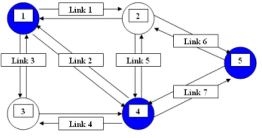
Figure 1. Illustrates road network.
The information given on picture network above to show example road network consist of seven link , five node ,six O-D pair, Travel time and Travel distance.
Travel distance of link1 = 100 km. Travel time of link1 = 3 hr. Travel distance of link2 = 150 km. Travel time of link2 = 3 hr. Travel distance of link3 = 200 km. Travel time of link3 = 4 hr. Travel distance of link4 = 200 km. Travel time of link4 = 3 hr. Travel distance of link5 = 100 km. Travel time of link5 = 3 hr. Travel distance of link6 = 100 km. Travel time of link6 = 4 hr. Travel distance of link7 = 100 km. Travel time of link7 = 2 hr. List of O-D pair
O-D of 1 to 4 = 1,200 veh. O-D of 1 to 5 = 2,200 veh. O-D of 4 to 1 = 900 veh. O-D of 4 to 5 = 1,100 veh. O-D of 5 to 1 = 1700 veh. O-D of 5 to 4 = 600 veh. List of population
The population of node 1 = 12,000 people. The population of node 4 = 4,000 people. The population of node 5 = 9,000 people. List of operating cost
VOC = 120 baht/veh-km. VOT = 210 baht/veh-hr.
From information above in this section presents the calculation of vulnerability measurements.
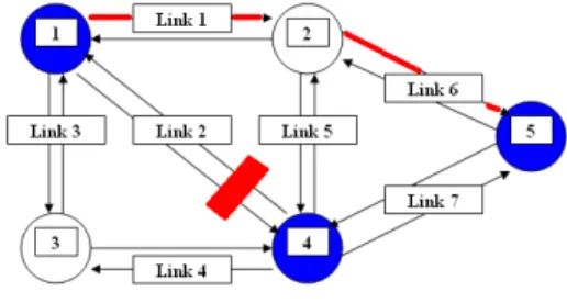
Example travel from node 1 to node 5. When full network
Figure 2. Illustrates the shortest route .
D15(G(N,L)) = 200 km. ( 125)
Figure 3. Illustrates the shortest travel time.
T15(G(N,L)) = 5 hr. (145) VKT15 = 200 × 2,200 = 440,000 km-veh VHT15 = 5 × 2,200 = 11,000 hr-veh TCD15 = 200 × 2,200 × 120 = 52,800,000 baht TCT15 = 5 × 2,200 × 210 = 2,310,000 baht AD15 = k (P1P5)/ T15(G(N,L)) 2200 = k(12,000 × 9,000)/ (5) K = (2,200)×(5) / (12,000 × 9,000) Example impact when link disruption When link 1 disruption
Figure 4. Illustrates the shortest route when link 1 disruption.
∆D15(L1) = 50 km. (Impact of travel distance)
Figure 5. Illustrates the shortest travel time when link 1 disruption.
∆T15(L1) = 0 hr. (Impact of travel time)
∆VKT15(L1) = 50 × 2,200 = 110,000 km-veh
∆VHT15(L1) = 0 × 2,200 = 0 hr-veh
∆TCD15(L1) = 50 × 2,200 × 120 = 13,200,000 baht
∆TCT15(L1) = 0 × 2,200 × 210 = 0 baht AD15(L1) = 2,200 veh.
∆AD15(L1) = 2,200 – 2,200 = 0 veh. When link 2 disruption
Figure 6. Illustrates the shortest route when link 2 disruption.
∆D15(L2) = 0 km. (Impact of travel distance)
Figure 7. Illustrates the shortest travel time when link 2 disruption.
∆T15(L2) = 2 hr. (Impact of travel time)
∆VKT15(L2) = 0 × 2,200 = 0 km-veh ∆VHT15(L2) = 2 × 2,200 = 4,400 hr-veh ∆TCD15(L2) = 0 × 2,200 × 120 = 0 baht ∆TCT15(L2) = 2 × 2,200 × 210 = 924,000 baht AD15(L2) = 1,571 veh. ∆AD15(L2) = 2,200 – 1,571 = 629 veh.
From the example of equations stated above, we can clearly measure impact of link disruption from the result of vulnerability index. When link one is disrupted, it will affect into around 50 kilometers
further than in normal route. Moreover it will rise up additional travel cost up to 13.2 million baht. When link two is disrupted, it will affect into travel time 2 hours further than in normal route. Moreover it will rise up additional estimated value of time at around 462,000 baht. After all it will end up with less demand on that route at around 629 vehicles from node 1 to node 5.
Table 1. Shows impact of O-D pair from node 1 to node 5 when link disruption.
Link
disruption (km.) ∆D15 ∆(hr) T15 (veh-km) ∆VKT15 ∆(veh-hr) VHT15
1 50 0 110,000 0 2 0 2 0 4,400 3 0 0 0 0 4 0 0 0 0 5 0 0 0 0 6 50 0 110,000 0 7 0 2 0 4,400
Table 2. Shows impact of O-D pair from node 1 to node 5 when link disruption (continue).
Link
disruption ∆(baht) TCD15 ∆(baht) TCT15 ∆(veh) AD15
1 13,200,000 0 0 2 0 924,000 629 3 0 0 0 4 0 0 0 5 0 0 0 6 13,200,000 0 0 7 0 924,000 629
4. Conclusion
All the suggested measurement factors stated might help the decision maker to answer the question of impact on different perspectives. By use the information giving on methods above to show on GIS , chat and plot graph to show the relationships between by comparing these pairs of information. - Compare ∆Dij(Ld) / Dij(G(N,L)) with Probability
of floods
- Compare ∆Tij(Ld) / Tij(G(N,L)) with Probability of floods
- Compare ∆VDTij(Ld) / VDTij(G(N,L)) with Probability of floods
- Compare ∆VTTij(Ld) / VTTij(G(N,L)) with Probability of floods
- Compare ∆TCDij / TCDij with Probability of floods
- Compare ∆TCTij / TCTij with Probability of floods
- Compare ∆ADij / ADij with Probability of floods From the information above, comparison will show the relationships of each indicator and equation. This will help the decision makers to work out with a clearer vision.
- If the result amount is located on the high-consequences and high-probability point, it might support the decision maker to solve the problem on that O-D pair urgently.
- If the result amount is located on the high-consequences but low-probability point, the decision maker might have to prepare to handle the problem on that O-D pair in advance since nowadays there are many unexpected incidents that can happen any minutes.
- If the result amount is located on the low-consequences but high-probability point, the decision maker still have to plan to organize with this O-D pair. However this point is not very urgent since the consequences rate is quite low, so the decision maker would know the important order of the problem as well.
- If the result amount is located on the low-consequences and low-probability point, the decision maker might consider solving problem on this point first. Since the closing for maintenance will not affect much to anyone.
The information above is just examples view for comparing the pair of O-D information but in real life it also depends on the decision maker who will use this information to organize the road network flow planning.
From the Method listed above, we will do the calculation and present by 3 system patterns included;
GIS
GIS will present the road network information with high Vulnerability index in each O-D pair from descending order on 7 views.
- Increase Travel Distance - Increase Travel Time
- Increase Vehicle Distance Traveled - Increase Vehicle Time Traveled
- ∆TCD (Increase Travel Cost base on Distance) - ∆TCT (Increase Travel Cost base on Time) - ∆ AD ( Decrease Accessibility Demand) Chart (column)
Chart (column) will present information by the plotting graph of comparison of consequences with the before and after of the disruption of the link. Chart (Column) will present in 5 different patterns as followed.
- Present Graph Compare between Increase Travel distance and Increase Travel time when the link is disrupted.
- Present Graph Compare between Increase Vehicle Distance Traveled and Increase Vehicle Time Traveled when the link is disrupted.
- Present Graph Compare between Increase Travel cost base travel distance and Increase Travel cost base travel time when the link is disrupted.
- Present Graph Compare between Accessibility before and after disruption link and show Decrease Accessibility.
Chart (XY Plot)
Five Chart (XY Plot) patterns below will present the calculated result of the Vulnerability index of the interested O-D pair by plotting into x and y axis. - Ratio Increase Travel Distance and Probability of floods
- Ratio Increase Travel Time and Probability of floods
- Ratio Increase Travel cost base travel distance and Probability of floods
- Ratio Increase Travel cost base travel time and Probability of floods
- Ratio Decrease Accessibility and Probability of floods
The three information presentation systems listed are expected result which is also our main objectives of this research.
References
[1] Abrahamsson, T., 1997. Characterization of vulnerability in the road transport system. Working Report TRITA-IP AR 97-53, Department of Infrastructure and Planning, KTH, Stockholm (in Swedish).
[2] Asakura, Y. 1999. Evaluation of network reliability using stochastic user equilibrium.
Journal of Advanced Transportation 33 (2),
pp.147-158.
[3] Bell, M.G.H. and Y. Iida. 1997. Transportation Network Analysis. Chichester: John Wiley and Sons.
[4] Bell, M.G.H.and C. Cassir (eds.). 2000.
Reliability of Transport Networks. Baldock,
Herts: Research Studies Press. Transport Network Vulnerability 29.
[5] Berdica, K., 2002a. An introduction to road vulnerability: what has been done, is done and should be done. Transport Policy 9, 117–127. [6] Chen, A., Yang, H., Lo, H.K. and Tang, W.H.
1999. A capacity related reliability for transportation networks. Journal of Advanced Transportation 33 (2), 183- 200.
[7] Chen, A., Yang, H., Lo, H.K., Tang, W.H., 2002. Capacity reliability of a road network: an assessment methodology and numerical results. Transportation Research Part B 36 (3), 225– 252.
[8] Chang, S.E. 2000. “Disasters and Transport Systems: Loss, Recovery, and Competition at the Port of Kobe after the 1995 Earthquake,” Journal of Transport Geography, Vol.8, No.1, pp.53-65.
[9] Dijkstra, E.W. 1959. “A note on two problems in connection with graphs.” Numerical Mathematics 1: 269-271.
[10] Department Of Highway. 2008. Prefeasibility Study and Initial Envirronment Examination for Executive Summary Report,70-71.
[11] FHWA. 1983. “Seismic Retrofitting Guidelines for Highway Bridges.” Report FWHA/RD83/007.
[12] Hansen, W.G. 1959. How accessibility shapes land use. Journal of the American Institute of Planners 25, 73-76.
[13] Husdal, J. 2004. Reliability and vulnerability versus costs and benefits. 2nd International Symposium on Transportation Network Reliability (INSTR2004): New Zealand.
[14] Holmgren,A ˚ ., 2004. Vulnerability analysis of electrical power delivery networks. Licentiate thesis TRITA-LWR LIC 2020, Department of Land and Water Resources Engineering, KTH, Stockholm.
[15] Immers, L.H., Stada, J.E., Yperman, I., Bleukx, A., 2004. Robustness and resilience of transportation networks. In: Proceedings of the 9th International Scientific Conference MOBILITA, Bratislava, Slovenia, May 6–7. [16] Iida Y, Bell MGH (eds) 2003 The network
reliability of transport. Pergamon-Elsevier, Oxford Koenig JG (1980) Indicators of urban accessibility: theory and application. Transportation 9:145–172.
[17] Jenelius, E. 2007. Incorporating dynamic and information in consequence model for road
network vulnerability analysis. INSTR 2007:
The Netherlands.
[18] Koenig, J.G. 1980. Indicators of urban accessibility: theory and application. Transportation 9, 145-172.
[19] Lam WHK (ed) 1999 Special issue on transport network reliability. J Adv Transp 33(2):121– 251
[20] Lam, W.H.K. and Xu, G. 2000. Calibration of traffic flow simulator for network reliability assessment. In Reliability of Transport Networks. Edited by M.G.H. Bell and C. Cassir. Baldock, Herts: Research Studies Press, 139-157.
[21] Morris, J.M., Dumble, P.L. and Wigan, M.R. 1979. Accessibility indicators for transport planning. Transportation Research 13A, 91-109.
[22] Nicholson, A.J., Du, Z.P., 1994. Improving network reliability: a framework. In: Proceedings of 17th Australian Road Research Board Conference, pp. 1–17.
[23] Nicholson, A. and Du, Z. P. (1997). ‘Degradable transportation systems: An integrated equilibrium model’. Transportation Research Part B, 31, pp.209-223.
[24] Nicholson, A.J. and Dalziell, E. 2003. Risk evaluation and management: a road network reliability study. In The Network Reliability of Transport. Edited by Y. Iida and M.G.H. Bell. Oxford: Pergamon-Elsevier, 45-59.
[25] Nicholson, A.J. and Dante, A. (eds.). 2004. Proceedings of the Second International Symposium on Transportation Network
Reliability (INSTR04). Department of Civil
Engineering, University of Canterbury, Christchurch, New Zealand.
[26] Niemeier, D. A. 1997. Accessibility: an evaluation using consumer welfare. Transportation 24, 377-396.
[27] Primerano, F. 2003. Towards a policy-sensitive accessibility measure. Papers of the
Australasian Transport Research Forum 27,
paper no 35, CD-ROM. Wellington: Transit New Zealand.
[28] Richardson, A.J. and Taylor, M.A.P. 1978. A study of travel time variability on commuter journeys. High Speed Ground Transportation Journal 12 (1), 77- 99.
[29] State of Minnesota. 2008. “Economic impacts of the I-35W bridge collapse.” Minnesota
Department of Employment and Economic Development, Minnesota Department of Transport. PM.
[30] Taylor MAP 1999 Dense network traffic models, travel time reliability and traffic management II: application to reliability. J Adv Transp 33(2):235–251 Taylor MAP (2000) Using network reliability concepts for traffic calming—permeability, approachability and tortuosity—in network design. In: Bell MGH, Cassir C (eds) Reliability of transport networks. Research Studies, Baldock, Herts, pp 217–242. [31] Taylor MAP, D’Este GM 2004a Critical
infrastructure and transport network vulnerability: developing a method for diagnosis and assessment. Proceedings of the Second International Symposium on Transportation Network Reliability (INSTR04). Department of Civil Engineering, University of Canterbury, Christchurch, pp 96–102.
[32] Yang, H., Lo, H.K. and Tang, W.H. 2000. Travel time versus capacity reliability of a road network. In Reliability of Transport Networks. Edited by M.G.H. Bell and C. Cassir. Baldock, Herts: Research Studies Press, 119-138.
[33] Nectec 2004 [Online], The Great Asian Earthquake and Tsunami 2004, Available : http://www.nectec.or.th/users/htk/20041226-quake/
[34] Thairath 2010 [Online], Road network Vulnerability in Khao Yai, Thailand, Available:
http://www.thairath.co.th/today/view/119426 [35] Thairath 2011 [Online], Flooding in South of
Thailand, Available : http://www.thairath.co.th/feed/4