Sibling Similarities, Differences and
Economic Inequality
Bhashkar Mazumder
Sibling Similarities, Differences and Economic Inequality
BHASHKAR MAZUMDER Federal Reserve Bank of Chicago
August 2004
JEL Codes: J0, D3, J62
Keywords: Sibling Correlation, Intergenerational Mobility, Sibling Inequality
Acknowledgements: I thank David I. Levine, Dan Sullivan and Kristin Butcher for helpful discussions and comments. I also greatly appreciate the outstanding research assistance provided by Sara Christopher.
Abstract: I use improved statistical approaches and much larger samples than previous studies to provide more robust estimates of the correlation in economic outcomes among siblings. A key finding is that more than half the variance in log wages among men is due to differences in family and community background. Slightly smaller estimates in the 0.45 to 0.5 range are found for earnings and family income. For women, the sibling correlation in family income is the same as that found for men. I estimate that the sibling correlation in years of schooling and AFQT test scores is higher than 0.6. In contrast, estimates for a variety of other non-economic outcomes (including physical attributes) are in the 0.2 to 0.4 range. Family and community influences are particularly important for those who start at the bottom of the income distribution. An analysis of the variance in outcomes within families, by quartiles of parent income provides a new set of facts that should inform theoretical models of family resource allocation. I also find that a large portion of the sibling correlation in some economic outcomes can be explained by observable characteristics.
1.
Introduction
How important are family background and community influences in determining economic success in the Unites States? The answer to this question will likely shape how we view the degree of economic mobility in American society. On the one hand, if family circumstances during childhood do not exert a large influence on one’s future labor market success, then it seems reasonable to conclude that there is a fair degree of economic mobility and equality of opportunity. On the other hand, if family and community influences strongly influence economic outcomes such as adult labor market earnings, then this at least raises the question of whether or not there is sufficient equality of opportunity in the U.S. and what, if anything, ought to be done about it.
A rapidly growing literature in economics has investigated the intergenerational mobility in economic status between parents and children by measuring the intergenerational elasticity in earnings or income. This line of research has made some important strides in documenting the strong persistence in economic outcomes across generations. However, the intergenerational elasticity has some limitations. First, from a conceptual point of view, it does not measure a broad range of family and community influences on children’s future outcomes. These factors are only captured to the extent that they are correlated with parents’ income. Second, there are many difficulties with empirical estimation since it requires collecting good data on the economic outcomes for two generations of individuals in the same family.
For these reasons an important alternative approach for measuring intergenerational mobility is to examine sibling correlations in economic outcomes. The sibling correlation answers the following
question: what percent of the variance in a particular outcome is due to factors that are common to growing up in the same family and community? This provides a broader measure of the overall importance of a wide variety of factors common to the family ranging from parental involvement to school and neighborhood quality – not just family income. Perhaps more importantly, it avoids many of the data problems that are inherent in intergenerational analysis by using contemporaneous accounts from
siblings who grew up together. The sibling correlation might also be more amenable to analyses that try to tease out the underlying factors that create strong intergenerational persistence in economic outcomes.
Only a few studies that I am aware of examine the sibling correlation in permanent economic outcomes in the U.S. using large national samples (Solon et al, 1991; Altonji and Dunn, 1991; Ashenfelter and Zimmerman, 1997; Bj`rklund et al, 2002). I improve upon these estimates in several ways. I employ variance component models using maximum likelihood that have desirable statistical properties – most importantly, consistency – lacking in previous analyses. I also use much larger samples containing many more siblings than previous work. I also examine more recent cohorts than previous studies. I present results on a variety of outcomes (earnings, family income, wages and hours worked) for both men and women. I also contrast the correlation in economic outcomes to the correlation in non-economic outcomes including measures of human capital, criminal activity, illegal drug use, physical attributes, health and psychological attitudes using the same sample.
A key finding is that sibling correlations in economic outcomes and human capital are larger than the correlations in a variety of other outcomes. It may be especially surprising to note that even measures of physical attributes such as height and weight which presumably have a strong genetic component, are not as highly associated between brothers as is the permanent component of wages.
In addition, I use this analytical framework to make progress in addressing other important questions. For example, how do families allocate resources between children? To what extent do families reinforce sibling differences or equalize them? Under certain assumptions theoretical models have clear predictions of how economic outcomes will differ among siblings depending on the permanent economic status of the parents (e.g. Becker and Tomes, 1976; Behrman et al, 1995; Dahan and Gaviria, 2003). Using a large sample of families I present new descriptive evidence of how sibling differences vary by initial family income and by racial group. These results present some interesting anomalies that ought to inform future work on this important question.
Finally I determine how much of the sibling correlation can be attributed to various observable characteristics in order to gain insight into the underlying forces that may cause a strong persistence in inequality across generations.
2.
Background and Literature Review
Why study the sibling correlation?
Conceptually, the sibling correlation in economic outcomes provides a summary statistic that captures all of the effects of sharing a common family. This may be contrasted with studies that only try to isolate the effect of family income or parent education on children’s future outcomes. If the similarity in say, wages between siblings is not much different compared to randomly chosen individuals, then we would expect a small correlation. If, however, a large fraction of the variance in wages is due to factors common to growing up in the same family environment then the correlation might be sizable. In that sense, the sibling correlation tells us how much of inequality is due to differences between families.
At the same time, the correlation among siblings does not only measure family background. It picks up all of the factors shared by siblings, not just having a common family. These may include the number of siblings, sharing the same neighborhood and school quality. Conversely, many aspects of family background will not be captured including genetic traits and parental behavior towards children that are sibling-specific. Overall, though, this measure is a useful way to characterize how important shared family and community characteristics are in explaining the overall variance in earnings.
Previous studies on sibling correlations in economic outcomes
An excellent review of economic studies on sibling correlations in economic outcomes is found in Solon (1999). I will briefly summarize that review. The estimates of brother correlations from studies that use only a singleyear of earnings for each sibling range from a low of .11 to a high of .44. The central tendency is about .25. Many of these studies use rather unique data sets that happen to track siblings from a particular community (e.g. Mormons in 19th century Utah) making it unclear how
representative these findings are. A homogeneous sample is also more likely to lead to attenuation bias because it will tend to have less “signal” in the data without a commensurate decline in the “noise” (Solon et al, 1991). The studies also differ in the age at which they collect data on income, which may have important effects on the results.
Solon (1999) also argues that when estimates of the brother correlation based on single year earnings are corrected for measurement error and transitory shocks, they should be scaled up by a factor of somewhere between 1.4 and 2.0. This suggests that the brother correlation in “permanent” status should be close to 0.4.
There are only four studies I am aware of which produce estimates of the sibling correlation in
permanent economic status. Two of these studies use the PSID and two use the NLS original cohorts. Solon et al. (1991) estimate the brother correlation in the permanent component of log annual earnings to be .34 when using the nationally representative portion of the PSID for the years covering 1975 to 1982. They estimate the brother correlation in log earnings at .45 when they include an oversample of poor families in the PSID and use weights.1 Similar results using the latter sample are found for other
outcomes such as family income. The highest estimate is 0.534 for log wages. Solon et al. also estimate the correlation among sisters in log income (0.276) and the log of the income to needs ratio (0.507).
More recently Bj`rklund et al (2002) have updated the PSID results of Solon et al (1991) in an attempt to compare the brother correlation in log annual earnings in the U.S. to several Nordic countries. They use the nationally representative portion of the PSID over the time period from 1977 to 1993 and their estimates of the brother correlation in earnings range between .42 and .45.
The methodological approach in both studies utilizes the random effects framework from the statistics literature and uses Analysis of Variance (ANOVA) formulas on regression adjusted log earnings to produce estimates of variance components. These are then used to produce estimates of the sibling correlation. In combination, these PSID results appear to support Solon’s conjecture that the brother correlation in permanent status in the U.S. is closer to 0.4 than 0.25.
With respect to the NLS, there are also two studies and both use only the original cohort of young men who are tracked from 1966 to 1981, roughly the same time period as covered by Solon et al.2 Altonji
and Dunn (1991) estimate the correlation in the permanent component of a variety of outcomes using two different methodological approaches to try to address the problem of transitory noise. First they use simple time averages of the outcome in question and calculate the covariance across all possible sibling pairs and divide this by the sample variance. Second, they use a method-of–moments approach that assumes that outcomes separated by at least a year are uncorrelated. For the brother correlation in log annual earnings their estimates are .32 and .37 and for log hourly wage their estimates are 0.33 and 0.42.
Ashenfelter and Zimmerman (1997) use the same NLS cohort to study the return to education and in a table describing their sample they report a brother correlation coefficient of .31 in log annual wages averaged over 1978 and 1981. It should be noted that all of the estimates from both studies using the NLS, include only individuals from multiple sibling families, use the oversample of black households, and do not include sampling weights. A reasonable reading of these results suggest that the brother correlation may be slightly more than 0.3 using the NLS data suggesting a possible discrepancy with the PSID results. On the other hand the NLS results are roughly in line with Solon et al’s finding of 0.34 when using the nationally representative portion of the PSID during a similar time period.
This study improves on the existing literature along several dimensions. I use much larger samples than previous studies and therefore provide more robust results. I use maximum likelihood estimators for variance component models that have more desirable statistical properties than ANOVA. I also apply a minimum distance estimator that has less strenuous data requirements as an alternative approach to dealing with serially correlated transitory shocks. Finally, I use data from a more recent cohort, the NLSY79, and look at both brothers and sisters for a variety of economic and non-economic outcomes.
1 This latter estimate also accounts for serial correlation in transitory shocks.
2 Oettinger (1999) uses the NLSY79 to study the sibling correlation in years of schooling and AFQT scores but does
In addition, there has been little empirical work by economists on understanding what factors drive the sibling correlation in economic outcomes. Altonji and Dunn (2000) find evidence of linkages between family members (including siblings) in unobserved preferences for work hours using a factor model. Solon Page and Duncan (2000) find that little of the sibling correlation in years of schooling can be explained by neighborhood effects. Neither study however, attempts to break down the sibling correlation in economic outcomes using a broad range of variables. Recent studies by Osbourne (2004), Heckman and Rubinstein (2001) and Dunifon, Duncan and Brooks-Gunn (2001) have demonstrated that there are important non-cognitive factors such as psychological attitudes that explain some of the intergenerational linkages in economic outcomes. I extend this kind of analysis to the study of sibling correlations.
Sibling differences and theories of family allocation
Previous analyses of sibling correlations in economic outcomes have typically assumed that the relationship among siblings is equally close for all families.3 However, the theoretical literature on the
allocation of resources within families suggests that there might be noticeable differences in sibling similarity across the income distribution. I begin by briefly summarizing some of the theoretical findings from Becker and Tomes (1976) and Behrman et al (1995) before discussing previous empirical work.
In the simplest case where parents are unconstrained in their ability to invest in their children’s human capital, they will invest in each child’s education until the marginal cost equals the marginal return. In this case, children who have higher returns perhaps because they have higher cognitive ability, will receive more schooling suggesting that we should observe differences in schooling and economic outcomes among siblings. If parents’ preferences are such that they would like to equalize the utility of their children, they compensate less able children with transfers and bequests.4
3 A notable exception is Oettinger (1999) who explores differences by parent education level and family size. 4 Behrman et al (1982) present evidence that families have an aversion to inequality among their offspring.
Families that face liquidity constraints, in contrast, may face an equity-efficiency tradeoff when dividing resources among children. Since they are unable to use transfers and bequests to equalize economic outcomes, parents who are averse to inequality may under-invest in children with high returns thereby creating more similar levels of human capital investment among siblings. This suggests that we would observe smaller (larger) differences in human capital and earnings among siblings who are raised in poorer (wealthier) families.
Dahan and Gaviria (2003) present a very different model that emphasizes increasing returns to human capital along with borrowing constraints. Under their model, poor families will find it
significantly more advantageous to invest all their resources in one child rather than under-invest in each child. This model suggests greater inequality among moderately poor families.
Since the sibling correlation provides a measure of sibling “similarity” it is tempting to infer that this measure may be used to evaluate these theoretical models since more “similar” siblings will be less unequal. Strictly speaking, however, these models have nothing to say about the sibling correlation per se, but do have a direct implication on measures that capture the variation in human capital and earnings within families. As I show in the next section, the use of a variance component model is ideally suited for such an analysis since it produces estimates of exactly what is needed –the variance that is due to
differences within families. Nonetheless, analyzing differences in the sibling correlation by parent income is also of interest since it may be informative as to where family background is most important.
Only a few previous studies have attempted to empirically examine sibling differences in human capital or economic outcomes distinguishing families by some measure of borrowing constraints.5 Gaviria (2002) uses the PSID and the HRS finds no significant difference in the average coefficient of variation across families in earnings (or education) by whether or not any sibling receives an inheritance. Gaviria’s PSID sample is relatively small and uses only earnings from a single year. His HRS sample
5 Behrman et al (1995) using the PSID present a simple table showing the mean, standard deviation and coefficient
of variation of absolute differences in earnings between siblings in two sibling families, by the number of siblings who have received transfers. However, the authors do not use the table to try to make any statements about the
uses responses from parents’ regarding their children’s earnings and schooling. Gaviria also doesn’t attempt to classify families by any other proxies for permanent income. Finally Gaviria doesn’t compare sibling differences in earnings with sibling differences in income, wages or hours.
Oettinger (1999) uses the NLSY79 and implements a multi-step procedure to produce an
observation specific estimate of the sibling correlation in schooling and AFQT test scores that controls for observable family and individual characteristics.6 He then regresses this measure on categories of
mother’s and father’s education as a proxy for permanent income. He finds that this measure of sibling similarity follows a U-shaped pattern in father’s education but that the differences are not statistically significant. As mentioned earlier, a preferred measure would be to simply use the variance within families rather than the sibling correlation. In addition rather than using father’s education, arguably a better proxy for parent’s permanent income would be to use parent income during the early years of the NLSY79 for the subset of siblings who lived with their parents. Finally, Oettinger does not examine economic outcomes or split the sample by gender.7
Statistical Models and Estimation Sibling Correlations: Base Model
I begin by discussing the method to estimate sibling correlations where I have multiple measures of the economic outcomes at different points in time. I start with a simple model where there is no persistence in transitory shocks.
(1) yijt = βXijt + εijt
The economic outcome (e.g. earnings) for sibling j, in family i in year t is denoted as yijt. Here, the vector
Xijt, contains age and year dummies to account for lifecycle effects and year effects such as business cycle
pattern of sibling differences by family type. They simply use the table to speculate as to the amount of inter vivos transfers or bequests needed to reconcile the model with the data.
6 Due to its complex design, it is not entirely obvious to this author that Oettinger’s measure is analogous to an
obsevation-specific measure of the sibling correlation.
conditions. These are considered fixed effects. The residual, εijt, which is purged of these effects is then
decomposed as follows:
(2) εijt = ai + uij + vijt
The three terms on the right hand side of (2) are considered random effects that are assumed to be independent of each other.8 The first term, a
i, is the permanent component that is common to all siblings
in family i. The second term, uij, is the permanent component that is individual-specific. vijt, represents
the transitory component that reflects noise due to either temporary shocks to earnings or measurement error in the survey. I begin by assuming that the transitory component is white noise. The variance of age-adjusted earnings, εijt, then is simply:
(3) σ2
ε = σ2a + σ2u + σ2v
The first term, σ2
a, captures the variance in permanent economic outcomes that is due to
differences between families while the second term, σ2u, captures the variance in permanent economic
outcomes within families. These two components are then used to calculate the correlation in permanent outcomes between siblings, ρ which is the focus of this analysis
(4) ρ = 2 2 2 u a a σ σ σ + ,
This is also equivalent to the fraction of the overall variance of the permanent components that is due to shared family and community background.9 Since σ2
u provides a measure of variation within families it
can be used to study theories of resource allocation by examining how the parameter changes depending on the initial income level of families.
8 The assumption that a
i and uij are uncorrelated is purely for analytical convenience and allows one conceptually, to
divide the permanent component into a part that is perfectly correlated among siblings, and a part that is perfectly uncorrelated among siblings. For the assumption that ai and vijt are uncorrelated I find (as did Solon et al, 1991) that
there is little or no cross-sectional correlation in the transitory component.
9 Conley (2004) has focused on the square of the correlation coefficient as a measure of explained variance since it
is equivalent to the R2 from a regression of one sibling on another. However, this captures the degree to which one
sibling explains the variance in the other sibling’s outcome, not the variance explained solely by the common family component. In my view this is not the correct way to measure the importance of family background since it includes information that is unrelated to family background. The appropriate R2 for analyzing the importance of family
Solon at al (1991) and Bj`rklund et al (2001) use a two step approach to estimate the variance components in this “mixed model” (mixed because it contains both fixed effects and random effects). First they use a regression to estimate (1) and to produce the residuals. Then they use classical analysis of variance (ANOVA) formulas that are adjusted for the fact that the data are “unbalanced” (the number of siblings varies by family and the number of available years varies by sibling).10 It is not clear, however,
that ANOVA is the preferred approach. Although ANOVA estimators of variance components have many desirable statistical properties for “balanced data”, virtually none of these properties transfer over to the case of unbalanced data (Searle et al, 1992). For this reason, many practitioners prefer to use
maximum likelihood techniques, which have a number of advantages such as consistency, asymptotic normality, and a known asymptotic sampling dispersion matrix.11 The main drawback of maximum likelihood is that it requires imposing a distributional assumption. Until recent years, computational limitations also made practical implementation of maximum likelihood more difficult.
Following the standard practice in the statistics literature I use a variation of maximum likelihood for mixed models called Restricted Maximum Likelihood (REML). REML partials out the fixed effects and maximizes the likelihood of the residuals containing the random effects variance-covariance
structure.12 A comforting feature of REML is that it produces identical results to ANOVA when the data
are balanced. I will present some results using both approaches to show that the results do not appear to be overly sensitive to the technique used. Another nice feature of REML is that it directly produces standard errors of the variance components.13 In addition, as I will show in the next subsection, REML
can more easily incorporate different assumptions about the time series properties of transitory shocks.
background is obtained from a regression of y on a. (were a available). As a result the square of the correlation coefficient is actually a downward biased estimate of the variance explained by family background.
10 These may be found in the Appendix of Solon et al (1991)
11 Searle et al (1992, page 254) conclude “It is our considered opinion that for unbalanced data each of ML and
REML are to be preferred over any ANOVA method.”
12 For a full textbook description of REML see for example, Searle Casella and McCulloch (1993). The analysis
here uses PROC MIXED in SAS.
Sibling Correlations: Model with Serially Correlated Transitory Component
I also consider the case where the transitory component is serially correlated and follows a first order autoregressive process:
(5) vijt = δ vijt + ξijt
One might expect that a failure to allow for serially correlated transitory shocks would result in variance component estimates that assign more of the persistent part of earnings to the permanent component, σ2
u
instead of σ2
v,. This would raise the denominator in (4) and could result in a lower estimate of ρ than
would be the case if the serial correlation were taken into account.
To address this I use two approaches. First I simply extend the REML framework to incorporate a first order auto correlation parameter and adjust the variance-covariance matrix accordingly. The only limitation of this approach is that it requires that the data contain consecutive years of information on the relevant outcome for each individual. In other words there can be no missing data within a string of years due to say, a missing survey year, non-response or a failure to meet sample selection rules. This is of some value when examining the NLSY79, which moved from annual surveys to biannual surveys after 1994.14
To address this issue and as a robustness check, I also employ a “minimum distance” (MD) approach that has been utilized extensively in the study of earnings dynamics (e.g. Abowd and Card, 1989; Baker, 1997; Haider, 2001) to distinguish the permanent component of earnings from the persistent transitory component. Here I exploit the autocovariance structure of earnings implied by the model to create a set of “moment conditions” that can be compared to the actual empirical moments calculated from the data in order to estimate the parameters of the model. This approach does not require dropping individuals who do not have consecutively ordered data.
I begin by combining the family component and the individual permanent component into one overall term α that represents the permanent component of earnings. This allows me to rewrite (2) as:
(6) εit = αi + vit
where i now indexes individuals and I no longer track families. Combining (6) and (7) I can write down the full autocovariance structure of earnings residuals. For example, the covariance between the earnings of individual i in year t, and his own earnings five years earlier can be written as follows:
(7) cov(εit,εit-5)= σ2α +
∑
= − 5 0 2 s v s s tσ
δ
The number of moments will depend on exactly how many years are available in the data. For T years of data, there will be (T X (T+1))/2 distinct moments. The empirical moments from the data are then stacked in a vector, M. The moment conditions implied by the model are viewed as a function of θ, or f(θ), where θ describes the parameters. The estimation procedure minimizes a distance function:
(8) D = [M- f(θˆ)]'W[M- f(θˆ)]
where is a positive definite weighting matrix. Following the recent literature, I use a variant of Equally Weighted Minimum Distance (EWMD) where the identity matrix is used as the weighting matrix.15
This provides an estimate of the overall permanent componentσ2
α, which is the denominator of
ρ. Of course, I still need an estimate of σ2
a, the family component in order to construct an estimate of the
sibling correlation. I do this by simply calculating the covariance in earnings between all pairs of brothers and across all possible earning-year combinations. I weight the sample by the inverse of the number of siblings to avoid “overweighting” families that contribute more observations (Solon et al, 2000).16
These approaches overcome the data limitations of the technique proposed by Solon et al (1991) and also employed by Bj`rklund et al (2001). Solon et al (1991) use differenced residuals to uncover an
14 This would be especially useful for researchers who wish to examine the original cohort of the NLS, which was
not surveyed annually.
15 Since I use unbalanced data I adjust the weighting matrix based on the proportion of non-missing data following
Haider (2001).
16 This is equivalent to Solon Page and Duncan’s weighting scheme (2) which produces estimates in the middle of
the range of all of their estimates. They find that the results are not very sensitive to the weighting scheme employed.
estimate of δ.17 They then implement ANOVA on the “delta-differenced residuals”. This method results
in losing one observation per individual and in dropping individuals who only have one year of available data. In addition, as with REML, Solon et al’s approach requires consecutive years of data.
Attributing the Sibling Correlation to Observable Characteristics
In order to understand how different observable characteristics (e.g. parent income, schooling) influence the sibling correlation in economic outcomes, I calculate an upper bound estimate of the contribution of various factors. I add the relevant variables to the vector X in (1) and treat them as additional fixed effects in the REML framework. The inclusion of additional fixed effects should sop up some of the residual variation in the outcome variable and produce lower estimates of the family
component (σ2*
a) than what was found without their inclusion (σ2a). I then take the reduction in the
variance of the family component (σ2
a - σ2*a) as an upper bound estimate of the amount of the overall
variance of the family component that can be explained by the specific factor(s) in question.18 The
change in the variance of the family component divided by the overall variance of the permanent component tells us what fraction of the overall sibling correlation is due to the factor(s) in question. Implementing this approach for a wide variety of possible explanatory variables, either by including them one at a time or all at once, should tell us something about which measures are critical to explaining the correlation in economic outcomes.
Sibling Correlation in Other Outcomes
I also investigate the sibling correlation in several non-economic outcomes where I do not need to examine multiple measurements at different points in time. This requires a far simpler model where I simply drop vijt from (2) and then use REML to simply calculate the two variance components σ2a and σ2u
in order to calculate ρ.
17 The residuals from (1) are first-differenced and the first difference is then regressed on its one period lag. The
resulting coefficient is transformed to create an estimate of δ.
18 This is an upper bound because it includes all omitted factors that are also correlated with the included fixed
effects. For example, the reduction in σ2
a due to the inclusion of years of schooling would be comprised of both the
direct effects of schooling as well as any omitted factors (e.g. perseverance) that also contribute to the outcome variable and are correlated with years of schooling.
In these cases I could consider a more straightforward approach to estimate the sibling correlation by simply calculating the correlation coefficient between all possible sibling pairs. However, this
technique would force me to eliminate all “singletons” (those without a sibling) from the analysis resulting in less efficient estimates of the family component. Another drawback to using sibling pairs is that the researcher must make a decision as to how to weight families because larger families will contribute many more sibling pairs (Solon et al, 2000). Nonetheless, as an additional check I also estimate the sibling correlation by following the methodology of Solon et al (2000). In this approach I calculate the covariance in years of schooling between all possible pairs of brothers, and calculate the variance in years of schooling for the sibling sample, and take the ratio of the two measures.19
3.
Data
The analysis uses the National Longitudinal Survey of Youth, (NLSY79) which followed
individuals between the ages of 14 and 21 on December 31, 1978 every year from 1979 through 1994 and then every other year. For economic outcomes, I use the NLSY data through the 1998 survey. The survey includes an oversample of black, Hispanic, and (non-black, non-Hispanic) disadvantaged families. However, the NLSY identifies a nationally representative cross section of families. I make use of the full sample by using survey year weights and also use the nationally representative sample without weights in some specifications.
I begin by identifying men and women between the ages of 14 and 22 in the initial survey in 1979. I examine four outcomes: log annual earnings, log annual family income, log hourly wages and log annual hours. The outcome variable must be observed and positive at least once when they are at least 26 years old and not enrolled in school.20 The NLSY identifies up to 5 siblings for each individual. An
obvious limitation of the dataset is that only siblings born within the eight year cohort window are
19 In calculating the covariance I weight the sample by the inverse of the number of siblings.
20 Earnings include earnings from wage and salaries as well as business income. I also imposed the following
sample restrictions for each outcome; earnings and family income had to be at least $500 in 1979 dollars; wages had to be at least $0.50 and no greater than $100; and annual hours had to be at least 100.
tracked. Second there is a potential problem with sample attrition, though the attrition rate is considerably lower than in the PSID.
I also examine a variety of non-economic outcomes with the NLSY and in some case include the 2000 survey, if relevant. For education, I examine years of completed schooling by age 26. For test scores I use the Armed Forces Qualifying Test (AFQT)21. Specifically, I use the percentile ranking for
the renormed (1989 version) score. For illegal drug use I use a 1988 survey question asking how many times the respondent has used marijuana or hashish in their lifetime. The responses are presented in 5 categorical groups. I use the type of residence variable from all survey years starting in 1983 to determine if individuals were ever in jail at the time of the interview. For women, I examine the age of first pregnancy (for the subset of women who were ever pregnant) and also an indicator of whether pregnant before age 20. I look at three measures of physical attributes, height (in 1985), weight at age 28 or 29 and body mass index (BMI).22 Finally, I look at two attitudinal measures from the psychology
literature. The first is the “Rotter scale” which measures the degree to which individuals feel they have control over their lives. Osbourne (2000) shows that this variable has an effect on the earnings of women. The second measure is a self-esteem scale, which combines responses to ten questions designed to
determine respondent’s views of self worth. In all the samples that examine non-economic outcomes, I require that observations not have missing data on the relevant outcome.
In most of the analysis the samples include siblings as well as non-siblings or “singletons” in estimating population variances. I do this to increase efficiency and to maintain comparability with Solon et al (1991) who had too small a sample of siblings to confine the analysis only to multiple sibling
families. Solon et al speculate that including singletons in the analysis may lead to an overestimate of ρ if
21 The AFQT is part of the Armed Services Vocational Aptitude Battery (ASVAB) given to applicants to the U.S.
military. The ASVAB consists of a battery of ten tests. The AFQT score is based on four of the tests that focus on reading skills and numeracy. The AFQT is a general measure of trainability in the military and is a primary criterion for enlistment eligibility. The test was administered to nearly all respondents in the NLSY in 1980 in order to provide new norms for the test based on a nationally representative sample. The AFQT is not viewed by the military or by most researchers as a measure of general intelligence or IQ.
22 Unfortunately height is only asked in 1985 so I am unable to control for age. However, the youngest respondents
outliers tend to be more common among singletons than siblings. This is because while singletons earnings are used to calculate σ2
a, the variance of the family component used in both the numerator and
denominator of ρ, they are not included in σ2
u, the variance of the individual component which is only in
the denominator of ρ. In the results that follow in the next section I conduct a wide range of robustness checks that include using a sample of only siblings.
For a subsample of the NLSY79, I have information on family income reported by the parents when the individuals lived at home. I use reported family income for 1978 and 1979 for this subsample to study differences in the sibling correlation and the within family variance by parent income level. A set of summary statistics is provided in Table 1.
4.
Sibling Correlations in Economic and Non-Economic Outcomes
Base Model for Economic Outcomes
I begin by presenting results where I do not allow for serially correlated transitory shocks. Since this is the first study to utilize the REML framework I start by contrasting a few selected results with those obtained by using ANOVA formulas. In Table 2 I present estimates of the variance components and the sibling correlation in annual earnings and hourly wages separately for brothers and sisters. Panel A shows the results for men and Panel B shows the results for women. The estimated brother correlations are 0.492 and 0.536 for earnings and wages, respectively. These results are similar to the higher set of estimates in Solon et al (1991) but are much more robust due to the significantly larger number of observations used. For example for men, Solon et al use around 2500 observations, 750 individuals and 600 families while this analysis uses 30,000 observations, 5000 individuals and 4000 families.
The results are lower for both outcomes when using ANOVA although the differences are not statistically significant. If REML produces more consistent estimates, then the consensus view of a sibling correlation in log earnings of around 0.4 expressed in Solon (1999) perhaps ought to be revised up to near 0.5. The results also suggest that the correlation in log wages appears to be higher than 0.5, which
is also consistent with Solon et al’s (1991) finding. In any case, these results reinforce the main point in Solon et al. (1991) that accounting for the transitory variance is critical –though at this point I have not yet examined the effects of serially correlated shocks. The implied correlation in wages, for example, were I to use data from just a single year would be just 0.306.
The results for the sister correlation in earnings and wages are somewhat lower at 0.340 and 0.360, respectively. This is not so surprising because women’s labor force participation patterns during their 20s and 30s are very different from men and may produce much noisier estimates of long-term economic status for these outcomes. Indeed, both the permanent individual component and the transitory components are dramatically higher than for men. I will look at the correlation in family income, a broader measure of economic status, in the next set of results. The ANOVA results are a bit lower for women’s earnings but are actually higher for women’s wages.
In Table 3, I confine the results to men and only present REML estimates. I present the same estimates for earnings and wages as in Table 2, but I now add family income and annual hours as additional outcomes. In column 1, I employ the base specification, which uses the full sample of men, including singletons and weights the sample with survey year weights. The brother correlation in family income is estimated to be 0.466 or slightly lower than the correlation in earnings, 0.492. Since family income includes spouse income it may be that assortative mating acts to lower the correlation between brothers in this outcome. The correlation in annual hours is estimated to be just under 0.4, which is similar to the reported results in Solon et al (1991) and the method of moment results in Altonji and Dunn (1991).
In Table 3 I also test whether the results are sensitive to the use of weights on the oversample of poorer families. In column 2 I use only the sample of families that are identified as nationally
representative in 1979. This results in keeping a little more than half the observations. The estimates drop only slightly for three of the four outcomes and are virtually identical for the fourth.
I also experiment with confining the sample to only individuals from families with multiple siblings. In column 3, I show that compared to column 1, the results are virtually identical when using a
sibling only sample. This is true even though only about a third of the total observations are used. In column 4, I combine both conditions (a nationally representative sample of only siblings). This strongly suggests that including singletons has little effect on the results.
In Table 4 I do the same analysis for women. The estimates for the correlation in family income among sisters are in indeed much higher than for the other outcomes. In fact, they are virtually identical to the correlation between brothers. For the nationally representative samples (columns 2 and 4), the correlation in family income is actually higher among sisters than among brothers (Table 3). The correlation in annual hours is very low but not surprising given the wide variance in labor force participation. Having established that with respect to the most comprehensive measure of economic status, family income, the sibling correlation is essentially the same for men and women, I proceed with the most of remaining analysis focusing just on men.
Model with Autocorrelated Errors
Thus far I have assumed that the transitory shocks are uncorrelated. I now assume that the transitory component follows an AR(1) process. As I discuss in section 2 both REML and the modified ANOVA approach require that the data must be consecutively ordered. Since ANOVA is done on differenced residuals this also requires dropping the first year for each individual. In Table 5, the first column shows the results from using REML. The estimates for the brother correlation in earnings (0.465), family income (0.439) and hours (0.322) are lower than what was found with the full sample in Table 3, while the estimate for wages (0.572) is higher. However, the differences from Table 3 are due to sample composition issues. I lose about one third of the person-year observations with the “consecutive sample”. In fact, running REML on this sample without the AR(1) results in estimates that are about 0.04 lower, on average, than the estimates in column 1 of Table 5. So including the AR(1) term (holding the sample constant) actually raises the estimates as I expected.
Using REML, the estimates for λ, ranges from around 0.35 to 0.37. This is roughly in line with previous estimates in Solon et al (1991) and virtually identical to the estimates found by Bj`rklund et al
(2002). I find that the estimates for this autoregressive parameter are near 0.3 irrespective of the outcome observed or the methodology used.
In column 2 I use the proposed minimum distance (MD) estimator on the same sample used in column 1 to isolate the effects of using a different methodology. For earnings and family income the estimates are close but they differ from REML quite a bit when examining wages and hours. The brother correlation in wages is now estimated to be 0.441 compared to 0.572 with REML. When I employ the MD estimator on the full sample that was used in Table 3 I find that the results go up for most outcomes and are now closer to the REML estimates in Table 3. The brother correlation in wages is estimated at 0.479, which is still very close to 0.5.
Finally, in column 4 I follow Solon et al (1991) and use ANOVA on the differenced residuals. The estimates for earnings (0.449) and family income (0.425) are lower than the REML and MD
estimates while the estimates for wages (0.567) and especially hours (0.501) are relatively high. One key drawback with this approach is that I lose many more observations.
The main point to take from this table is that after accounting for sample composition, the results are fairly similar and perhaps slightly higher when I account for autocorrelated shocks to earnings. . In addition, I find that compared to REML our MD approach leads to roughly similar results for three of the four outcomes, the exception is wages where MD results in a significantly lower estimate. These results provide confidence in using the MD approach when using data that contains missing survey years and where it is important to account for autocorrelated transitory shocks.
Sibling Correlations in Non Economic Outcomes
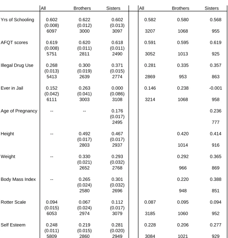
Table 6 presents the results for a variety of non-economic outcomes for brothers, sisters and all siblings as appropriate. This serves as a useful point of contrast with the economic outcomes and is also interesting in its own right. I use much larger samples than previous studies and extend the components of variance approach using REML. In contrast to most previous work I do not need to rely on samples consisting only of sibling pairs although I do present results using this approach. The first three columns
use the REML approach including singletons while the fourth through sixth columns use only sibling pairs, and follow the methodology employed by Solon et al (2000) described earlier. I will refer to this approach as “SPD” (for Solon, Page and Duncan). In both cases I use only the nationally representative portion of the NLSY.23
The correlation in years of schooling appears to be roughly similar for both brothers and sisters and the correlation across all sibling pairs is about 0.6. When I use the SPD approach I get slightly lower estimates that are roughly in line with the results in Solon et al (2000) who use the nationally
representative portion of the PSID. For AFQT scores, the estimates are also similar across genders and are even higher than the education estimates.
I next focus on a few socioeconomic outcomes that have been commonly analyzed in studies of neighborhood/peer effects (e.g. Case and Katz, 1991). I find that the correlation in drug use among all siblings is a bit below 0.3. However, there does appear to be a significantly higher correlation among sisters (0.37 using REML) than brothers (0.3). The fact that the overall correlation is lower than the correlation within gender type suggests that the correlation across siblings of different genders is lower. When I examine whether respondents were ever in jail, I find that the correlation is actually slightly negative using SPD. Since variance component models, by definition, are bounded at zero, the REML estimate for sisters is zero. For brothers the correlation estimates are around 0.25. Finally, the correlation in age at pregnancy is less than 0.2 when I use REML but slightly greater than 0.2 using SPD.
I now turn to physical characteristics/health outcomes. When I use REML, the correlation in height between siblings is slightly below 0.5. The estimates are closer to 0.4 when I use SPD. The estimates for weight are around 0.3 for brothers and sisters using REML. The SPD estimates, however, are quite a bit higher for sisters. Similarly for BMI I find that the correlation among sisters is higher than
23 Including the oversample of poorer and minority households without weights results in similar estimates. I found,
however, that when I used weights with REML on the non-economic outcomes it sometimes led to very large estimates of ρ that seemed implausible. Therefore, I chose to only use the representative sample without weights when studying non-economic outcomes.
among brothers using either method. Finally, with the attitudinal variables, the correlation in the Rotter scale is only about 0.1 in all cases while the correlation in self esteem is in the 0.2. to 0.3 range.
Overall, it appears that the correlations in the human capital measures are actually the highest at around 0.6. Otherwise, the only variable with a sibling correlation comparable to the economic outcomes is height. This further points to the fact that economic status in particular is strongly influenced by family and community factors.
5.
Sibling Inequality and Resource Allocation
I now examine the extent to which sibling similarities and differences vary by parents’ economic status and how this might influence theories of resource allocation within families. For this analysis I use a subset of families for whom parents in the NLSY answered questions about the income received in 1978 and 1979.24 The two-year inflation adjusted average of parent income is then used to split the
sample in order to identify groups of families that should experience varying degrees of borrowing constraints. In this exercise I present results on the correlation as well as the individual component, σ2u,
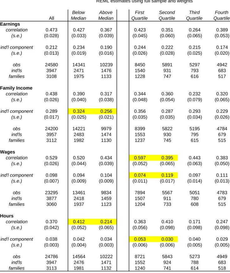
which captures the variation within families. The results for men’s economic outcomes are shown in Table 7.
The first column shows the results for the whole sample with available information on parent income. The next two columns show the results when the sample is split at the median level of parent income.25 The last four columns show the results by quartile of parent income. It is immediately evident
that for all four economic outcomes, the correlation is higher for families whose parents had below median income compared to those with above median parent income although only in the case of hours is the difference statistically significant. Still, this provides some fairly suggestive evidence that family background is especially important for families in the lower half of the distribution.
24 Footnote explaining NLSY income
Looking across the quartiles, the highest estimates are in the bottom quartile for wages and earnings. For wages, the difference between the first two quartiles is especially large and is statistically significant. The brother correlation in wages is close to 0.6 for families in the bottom quartile. For family income and hours the estimates for the second quartile are slightly higher. For hours the difference is statistically significant. This suggest that while the correlation in annual earnings is roughly equal between the first two quartiles that this masks underlying differences in the correlation in wages and hours worked.
There is evidence of an increase in the correlation for the top quartile for three of the four
outcomes, but in no case are the differences between the third and fourth quartiles statistically significant. No other obvious patterns are detected that are consistent across the outcomes.
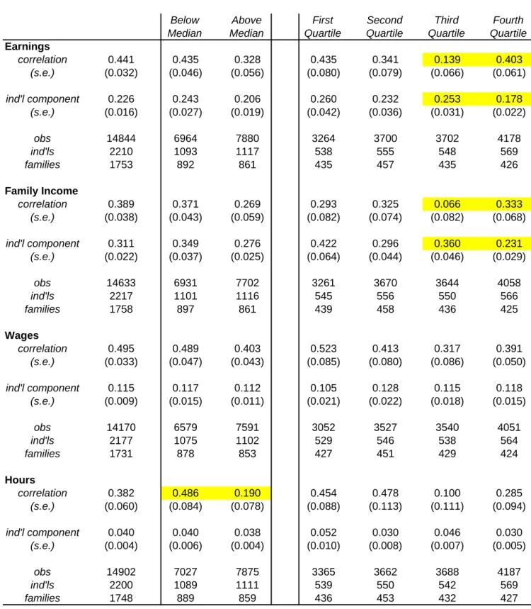
As an additional check, I also examined the estimates using the nationally representative sample without weights where the sub-samples are now more evenly split across the four quartiles. These are shown in Panel B of Table 7. With this sample I once again observe that the correlation is higher among below median families than above median families for all four outcomes. But also as before, the
difference is only significant for hours. With these samples there is stronger evidence of an increase in the correlation among the top quartiles for all four economic outcomes. The differences are now statistically significant for earnings and family income. Overall, the evidence strongly suggests that family background is particularly important at the low end of the income distribution but also suggests that family differences are pronounced at the top of the distribution.
As noted earlier, it is incorrect to infer that since sibling similarity in economic outcomes (as measured by the sibling correlation) is highest for the bottom quartile that it necessarily follows that sibling differences within families, are smallest for this group. Recall, that the sibling correlation for a particular subgroup essentially scales that “between family” component of variance (σ2
a), relative to the
overall variance for that subgroup (σ2
a.+σ2u). If the magnitude of differences between families varies
across the quartiles of the income distribution but the magnitude of differences within families does not, then I could observe variation in the sibling correlation across quartiles but observe no variation in the
within family variance component. Note that it is the latter parameter that is more relevant for the theoretical models.
In fact, Table 7 also shows that the estimates for the individual component, which measures the variance within families in permanent outcomes, do not follow a consistent pattern across the four economic outcomes. For earnings, there appears to be almost no difference in the variance within
families across the parent income distribution. Still, there is some sketchy evidence that is consistent with the theoretical models. Specifically, it appears that sibling differences in wages are very small in the bottom quartile of parent income while sibling differences in family income are relatively small in the top quartile. This is roughly consistent with the idea that poorer families may be forced to choose equity over efficiency while wealthier families are able to reinforce sibling differences in ability through human capital investments but compensate less able siblings through transfers. I will provide more insight on this shortly when I examine inequality in years of schooling and test scores. It also appears that the within family variance in hours worked is especially high for families in the bottom quartile which explains why the greater equality in wages among siblings in the bottom quartile is not reflected in greater equality in annual earnings.
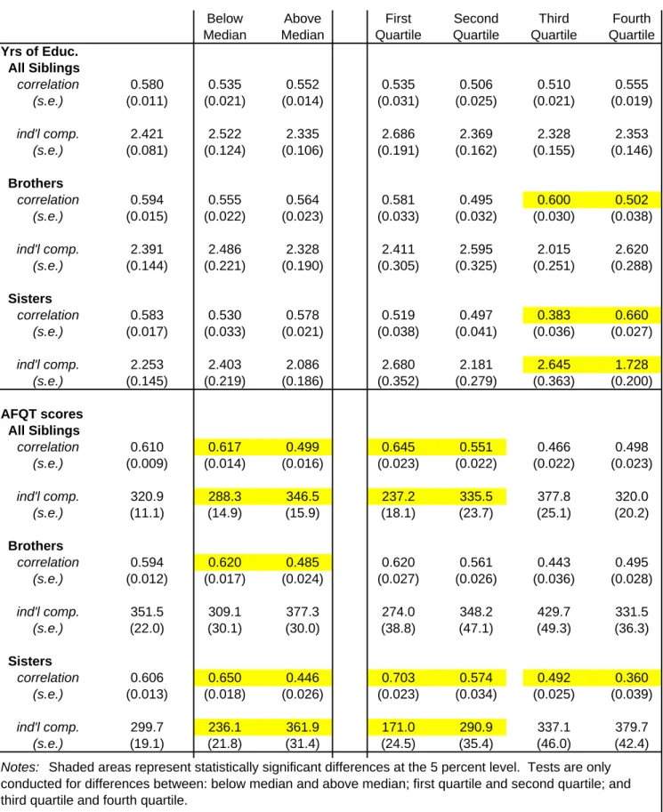
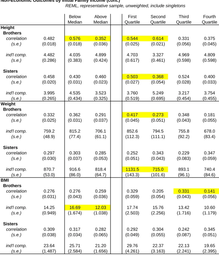
In Table 8, I examine differences in the sibling correlation and the within family variation for a few non-economic outcomes. Specifically I examine measures of human capital, education and AFQT scores, which should have direct bearing on theoretical models. These are also contrasted with results for a few physical characteristics, height, weight and BMI for which we may not have any pre-conceived idea of how the estimates might differ across the parent income distribution. I also examine both brothers and sisters and both genders combined for the human capital outcomes. Some previous studies (e.g. Butcher and Case, 1992) have found that gender composition of families may effect intra-family resource allocation.
Looking first at education, there is no evidence that there is any significant difference in either the correlation or the within family variance when I combine men and women. The only noticeable
For brothers the correlation is significantly lower for the top quartile than the third quartile. The variance within families is also a bit higher (though not significant) for the top quartile compared to the third quartile but not much different from the first and second quartiles. Interestingly, for women, the reverse pattern holds. The correlation rises sharply for the top quartile and is statistically significant while the within family variation drops sharply for this group. This appears to suggest that there are gender-specific differences in human capital investment among wealthier families.
For AFQT scores, the differences are far more striking and accord more closely with the patterns in men’s economic outcomes. The correlation in AFQT scores is significantly higher for families with below median parent income compared to above median families. This is true whether I examine all siblings or look at brothers or sisters independently. For example, for sisters growing up in families in the bottom quartile the correlation is a stunning 0.7. The within family variation is also significantly lower for families in the bottom half of the distribution. In fact, inequality appears to rise with income for both sexes.26 This conforms to the Becker-Tomes model where richer families are able to invest more
efficiently in their children’s human capital leading to more unequal outcomes. For the top quartile, however, there is a noticeable break in the pattern by gender. Unlike the case with years of schooling, there is more equality in test scores among brothers and less equality among sisters.
These results raise at least two interesting questions. First, why are there differences between schooling and AFQT scores? Second, why do the patterns differ by gender? With respect to the first point, it could be that parents use different strategies for human capital investment depending on how observable their actions are. This could be due to reasons of fairness and/or social norms. For example, society may perceive parents who send only one of their two children to college as acting unfairly. In contrast, choosing to read more books to a child who appears to have greater potential scholastic ability (and who may enjoy school more) may not seem so unfair. The disparity in AFQT scores among siblings may capture differences in parent investment in children’s cognitive ability that are not easily observed. Given that the data on education doesn’t appear to fit the standard models this seems to be an explanation
that ought to be examined more closely. With respect to the second question, this study does not offer any new insight but simply provides more evidence suggesting that there appear to be gender differences at play in family resource allocation decisions.
Table 8 also examines differences across the income distribution in the sibling correlation and within family variation with respect to height, weight and BMI. These are examined separately for brothers and sisters. For 5 of the 6 cases, the estimate for the sibling correlation is higher for families with below median parent income. But in only one case (men’s height) is the difference statistically significant. Looking at the sibling correlation by quartiles there are really no consistent patterns. For two of the outcomes (sister’s height and men’s weight) the difference in the correlation is significantly higher for families in the bottom quartile compared to the second quartile but in other cases the second quartile estimate is higher. Overall, the results provide some weak evidence that for physical characteristics family background appears to be more important at the low end of the distribution.
There is also evidence that there is greater inequality within families at the low end of the distribution. For 5 of the 6 outcomes, the variation within families is higher for families with below median parent income but in only one case (men’s BMI) is the difference statistically significant. Similarly, for 5 of the 6 cases the variation is higher for families in the bottom quartile compared to the second quartile but again only in one case is the difference statistically significant. Interestingly, for 5 of the 6 outcomes there appears to be a decline in inequality as families move from the third quartile to the top quartile. However, in no case is the difference statistically significant.
A comparison between the economic outcomes, human capital measures and physical
characteristics across the parent income distribution, suggests the following. Across nearly all outcomes the sibling correlation tends to be higher in the bottom half of the distribution and generally in the bottom quartile. This is particularly pronounced, however, with respect to AFQT scores and wages. This suggests that while family and community influences are generally important for poorer families they are particularly important in determining skill levels and wages. This pattern is still evident though much
more muted when examining years of schooling. This is not so surprising given that for this cohort compulsory schooling has probably made differences in the correlation by income level much weaker.
Comparisons across the various outcomes also offer some mixed evidence in support of the theoretical models of intra-family resource allocation that emphasize parental aversion to inequality, ability differences among siblings and borrowing constraints. As these models imply, I find evidence of higher inequality in test scores and wages among better-off families and less inequality in family income. On the other hand, the variation in years of schooling across the parent income distribution does not fit the expected pattern as neatly. This raises the possibility that there might be differences in how parents use observable versus unobservable forms of human capital investment. There also appear to be clear differences in how parents invest in their children by gender. Finally, previous studies that have solely focused on the within family variation in annual earnings may have overlooked the importance of labor supply effects that might have obscured the relationship between parent income level and sibling inequality in hourly wages.
Examining physical characteristics suggests that inequality within families appears to be higher in the lower end of the distribution. This suggests that the patterns observed with respect to some of the human capital and economic outcomes are unique and not found for other outcomes for which we are less likely to have any prior belief about how inequality might vary across the distribution.
6.
Sibling Correlation and Inequality by Race
Most previous studies have had insufficient samples to study sibling similarity by race or ethnic group. At a general level, it would be interesting to know the extent to which the overall differences between families are due to differences across racial groups. Does family background matter just as much in white families as in black families? Examining differences between families within racial or ethnic minorities could also offer greater insight into the factors that might generate inequality between families. For example, if the sibling correlation is higher for minority groups who tend to live in geographically concentrated areas it could reflect a greater role for community influences (e.g. Borjas,
1992). Also analyzing differences within racial groups might also serve as an additional check on the results related to differences by parent income level. In other words, is the finding that family
background matters more for families starting at the bottom of the income distribution really just picking up the effects of race or ethnicity? Finally, given the central importance of the black-white gap in earnings, assembling the basic facts on family inequality by race should be of interest in its own right.
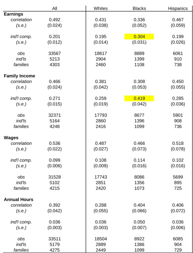
Table 9 presents the results for economic outcomes. The sibling correlation appears to be quite a bit lower for blacks than whites for both earnings and family income although the differences are not statistically significant different from zero. Unfortunately, even with the larger samples available with the NLSY, the standard errors are too high to detect meaningful differences. The white-black difference in the correlation in wages appears to be negligible and the magnitudes of the correlation for each group are only slightly lower than for the whole sample. This suggests that the earlier finding that about half the variance in men’s wages is due to family and community influences, is not due to race. Interestingly, the correlation in hours is sharply higher for blacks but also not statistically significant.
In contrast, the brother correlation in earnings, family income and wages among Hispanic families are slightly higher than for whites, though in no case are the differences statistically significant. The correlation in hours worked is quite a bit higher for Hispanics than whites and is almost identical to that found for blacks.
Looking at the individual variance component by race shows much greater inequality in earnings and family income in black families. For example, the variance in family income within white families is 0.259 compared to 0.419 for black families. These differences are statistically significant. The black-white gap in sibling wage inequality is much more muted. So to a large extent, greater sibling inequality in earnings among blacks is driven by differences in labor supply. The pattern in sibling inequality among Hispanic families appears to be virtually identical to whites.
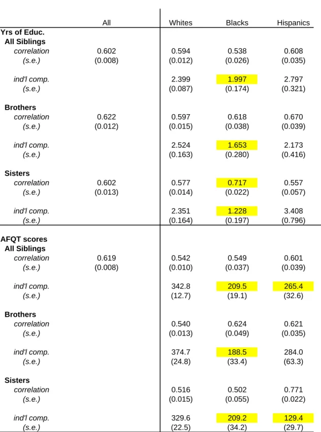
Table 10 presents the analogous results for human capital measures. For education there are no statistically significant differences in the sibling correlation when all siblings are pooled irrespective of gender. The variation in education within families however is significantly lower for blacks. This result
fits the basic spirit of the Becker-Tomes model where there is greater equality among poorer families that are presumably borrowing constrained. It appears that while the tendency to equalize schooling levels is not characteristic of families with low parent income it does seem to characterize black families. Looking at the samples of brothers and sisters, separately, I now find that the correlation is higher among blacks and that the difference with whites in the sister correlation is statistically significant. This seeming discrepancy with the results when pooling brothers and sisters suggests that the cross-gender correlation is lower among blacks –pointing to yet another example where gender differences appear to matter. The finding that sibling inequality is lower for black families also holds up when examining brothers and sisters separately. For Hispanics, there are no significant differences with whites although the correlations differ substantially by gender.
For AFQT test scores, in no case are the white-minority differences in sibling correlations
statistically significant. As with education, sibling inequality is found to be much lower in black families. Interestingly, for Hispanic families, I now find that the variation among siblings is also significantly lower than for whites. These results are more in line with the Becker-Tomes model and also appear to be consistent with the results in Table 8. One stunning finding is that the estimate for the correlation in test scores among Hispanic sisters is 0.77. The results for physical characteristics (not shown) do not exhibit the same patterns as the human capital outcomes.
Overall, the results for race raise more questions for the theoretical models. While there is evidence of less inequality in human capital investments among minority families this does not appear to translate into lower sibling inequality in wages. The sharp differences in sibling inequality within racial groups by gender, also raise concerns about the adequacy of the theoretical models.
7.
Contributions to the Brother Correlation in Economic Outcomes
I now examine the potential impact of various explanatory variables on the sibling correlation in economic outcomes among men. In Table 11 results are presented that show upper bound estimates of the contribution of various variables using the methodology described in section 2. One obvious
candidate for explaining the sibling correlation is parent income. With the NLSY79 sample there is only information for a subset of individuals for just a few years on parent income. As Solon (1992) has shown, using income from just a single year is a poor proxy for permanent income and leads to downward biased coefficients. Similarly, using just a two-year average of income from 1978-79 will also likely to lead to biased estimates of the residuals (purged of parent income), and therefore, biased estimates of the variance components. In any case using this proxy for parent permanent income I find that the variance in the family component in earnings residuals is reduced by 0.17, which explains about 36 percent of the sibling correlation in earnings.27 The contribution to the sibling correlation in family income is slightly
higher at 41 percent but the contributions to the sibling correlations in wages and hours are 27 percent and 21 percent, respectively.
I next examine how the two measures of human capital used earlier, years of schooling and AFQT scores, influence the sibling correlation. Both measures fare almost equally well in explaining the sibling correlation in various outcomes. For earnings, family income and wages, each measures explains anywhere between 40 and 50 percent of the sibling correlation. Including both human capital measures in conjunction explains more than half of the sibling correlation in earnings and family income. These human capital measures, however, only explain about 20 percent of sibling correlation in annual hours.
Physical characteristics only account for about 5 percent of the sibling correlation, most of which is due to the inclusion of height. Accounting for any time spent in jail explains more than 20 percent of the sibling correlation in earnings, family income and hours but less than 10 percent of the sibling correlation in hourly wages. Illegal drug use, however, appears to explain virtually none of the sibling correlation. Both psychological measures make an important contribution to explaining the sibling correlation in earnings, family income and wages. Combined, they account for about 20 percent of the sibling correlation in these measures. This result adds to the growing number of studies that have found
27 Solon (1999) shows that using the consensus estimates of the intergenerational elasticity in earnings of 0.4, one
would expect the contribution to be (0.4)2 or 0.16. If, however, the intergenerational elasticity is actually closer to