issn1091-9856eissn1526-55281022010154 doi10.1287/ijoc.1090.0317 © 2010 INFORMS
Binarized Support Vector Machines
Emilio Carrizosa
Departamento de Estadística e Investigación Operativa, Universidad de Sevilla, 41012 Sevilla, Spain, [email protected]
Belen Martin-Barragan
Departamento de Estadística, Universidad Carlos III de Madrid, 28903 Getafe, Madrid, Spain, [email protected]
Dolores Romero Morales
Saïd Business School, University of Oxford, Oxford OX1 1HP, United Kingdom, [email protected]
T
he widely used support vector machine (SVM) method has shown to yield very good results in super-vised classification problems. Other methods such as classification trees have become more popular among practitioners than SVM thanks to their interpretability, which is an important issue in data mining.In this work, we propose an SVM-based method that automatically detects the most important predictor vari-ables and the role they play in the classifier. In particular, the proposed method is able to detect those values and intervals that are critical for the classification. The method involves the optimization of a linear programming problem in the spirit of the Lasso method with a large number of decision variables. The numerical experience reported shows that a rather direct use of the standard column generation strategy leads to a classification method that, in terms of classification ability, is competitive against the standard linear SVM and classification trees. Moreover, the proposed method is robust; i.e., it is stable in the presence of outliers and invariant to change of scale or measurement units of the predictor variables.
When the complexity of the classifier is an important issue, a wrapper feature selection method is applied, yielding simpler but still competitive classifiers.
Key words: supervised classification; binarization; column generation; support vector machines
History: Accepted by Amit Basu, former Area Editor for Knowledge and Data Management; received February 2006; revised January 2008, July 2008; accepted December 2008. Published online inArticles in Advance April 7, 2009.
1. Introduction and Literature Review
Classifying objects or individuals into different classes or groups is one of the aims of data mining. This topic has been addressed in different areas such as statistics, operations research, and artificial intelligence. A gen-eral introduction of data mining can be found in Hand et al. (2001).
We focus on the well-known so-called supervised classification problem, usually referred as discrimi-nant analysis by statisticians, where we have a set of objects and the aim is to build a classification rule that predicts the class membership cu of an object u
into one of a predefined set of classes by means of its predictor vector xu. The predictor vector x takes
values in a set X, which is usually assumed to be a subset of p, such as 01 p. The components x
l, l=12 p, of the predictor vectorxare called pre-dictor variables. The other piece of information defin-ing uis the classcu to which objectubelongs. In this
paper, we restrict ourselves to the case in which two classes exist,=−11 , since the multiclass case can be reduced to a series of two-class problems, as has
been suggested, e.g., in Hastie and Tibshirani (1998), Herbrich (2002), and Vapnik (1998).
Information about the objects inis available only in a subset I, called the training sample, where both predictor vector and class-membership of the objects are known. With this information, the classification rule must be built.
The support vector machines (SVM) (Cortes and Vapnik 1995) approach is based on margin maximiza-tion, which consists in finding the separating hyper-plane that is farthest from the closest object. SVM has been shown to be a very powerful tool for super-vised classification. The most popular versions of SVM embed, via a kernel function, the original predictor variables into a higher (possibly infinite) dimensional space (Herbrich 2002). In this way, one obtains classi-fiers with good generalization properties but, in gen-eral, can be hard to interpret.
In some application fields, practitioners such as doctors or businessmen may be very unwilling to use a classifier they cannot interpret. For them, data mining methods sometimes proceed like a black box, 154
so they would not feel confident enough to use clas-sifiers unless they can interpret them somehow.
For instance, it is easy to interpret and manage queries such as
• Is predictor variablel1 big? • Is predictor variablel2 small?
• Does predictor variable l3 attain a very extreme value?
In these queries, the concept of “big,” “small,” and “extreme value” must be quantified, e.g., in the form Is predictor variablelgreater than or equal tob? (1) This type of query is used, e.g., in classification trees (CART). Because of its very intuitive graphical display, practitioners can interpret the classifier and describe how it works. Moreover, they can detect the values of a predictor variable critical for the classification.
In this paper, we work in an SVM-based framework where the feature space is defined by binarizing each predictor variable, i.e., by transforming each numer-ical predictor variable l into a large series of binary variables, obtained by making queries of type (1) for many different cutoffs b. Because we are using SVM after binarizing the predictor variables, we call our method binarized support vector machines (BSVM).
Our aim is to show that if SVM is run after such binarization, the resulting classifier has valuable prop-erties concerning classification ability, interpretability, and robustness.
First, the numerical experience reported in §4 shows that BSVM yields lower misclassification rates than classification trees and is competitive (in other words, better in most cases we tested) against linear SVM.
Second, BSVM takes us a step forward toward interpretability of SVMs. Because the obtained classi-fication rule is based on queries of type (1), the criti-cal values and intervals of the predictor variables are identified, as done by classification trees.
Third, BSVM is linear in the sense that it yields a classification rule that is linear in the features selected, and it can be seen as a linear SVM after transforming the variables via a nonlinear mapping. Such mapping, which can be visualized by means of a graphical pro-cedure, is valuable in terms of interpretability because it shows the way each predictor variable influences the classifier. The capability of BSVM to capture non-linearities presents an advantage with respect to the standard linear SVM, with important consequences in the classification ability as shown in our numerical results.
Finally, the use of queries of type (1) in our method makes it appealing in terms of robustness against out-liers and changes of scale in the data. The numer-ical experience reported shows that our procedure behaves as classification trees and clearly better than
linear SVMs in the presence of outliers. Moreover, whereas the linear SVM is influenced by the scale in the data—even a linear change of scale in the predic-tor variables may change the classifier and thus the classification ability of the SVM methodology—our proposal yields a classifier that is invariant to change of scale, in the sense that if the data were modified by a monotonic (non)linear transformation, the classifier obtained would be the same.
Note that the binarization procedure as proposed in this paper is applied to each predictor variable sepa-rately. Hence, interactions between predictor variables are not taken into account. Introducing them in the model adds extra computational complexity that is outside the scope of this paper.
The idea of binarizing continuous predictor vari-ables is not new at all in the field of classifica-tion. Indeed, classification trees are precisely based on the strategy of defining, for different predictor variables, appropriate cutoffs. Moreover, binarizing is also natural in other classification procedures such as neural networks, where the well-known step activa-tion funcactiva-tion, already at the heart of the perceptron method, allows one to discretize any predictor vari-able or combination of them. Binarizing continuous predictor variables has also been proposed in the so-called rule extraction procedures within SVM (Barakat and Diederich 2004, 2005; Fung et al. 2005; Martens et al. 2007; Núñez et al. 2002) and neural networks (Andrews et al. 1995, Baesens et al. 2003, Craven and Shavlik 1997). When a rule extraction method is applied to a classifier, one obtains an alternative clas-sifier that hopefully has a similar behavior on data but is moreinterpretablebecause it is based on simple rules such as those derived from queries of type (1). Whereas our method shares with rule extraction pro-cedures the aim of enhancing interpretability of the output of an SVM, we are not proposing to replace the SVM classifier by a more interpretable one that, based on queries of type (1), mimics the behavior of the SVM classifier; instead, we are proposing a binariza-tion in the data via queries of type (1) and by obtain-ing the SVM classifier for such transformed data. This way, we increase interpretability with respect to stan-dard SVM and, as shown in our numerical experience, provide a competitive method in terms of misclassifi-cation rates.
As far as we are aware, there is no paper using this way binarization for support vector machines; thus, our strategy is new in the context of SVM.
The classifier proposed in this paper, BSVM, is de-scribed in §2, where we analyze the interpretability of the proposed method and propose a visualization tool for plotting the role of a predictor variable in the classifier. Because the number of features to be con-sidered may be huge, the BSVM method yields an
optimization problem with a large number of decision variables. In §3, a column generation-based algorithm is proposed to solve such an optimization problem. Numerical results are presented in §4; they illustrate the classification ability and the desirable properties of BSVM, and show that the proposed approach gives a classifier that is competitive against the standard lin-ear SVM or classification trees. When the complexity of the classifier is an important issue, a wrapper fea-ture selection method is applied to reduce the number of features used in the classifier at the expense of a mild loss in the classification ability. Conclusions and some lines for future research are discussed in §5.
2. Binarized Support Vector Machines
Queries of type (1) are simple and, hence, are by themselves easy to interpret. In §2.1, we introduce a classifier that is made up by queries of this type. We propose in §2.2 a visualization tool that graphi-cally represents the role any original predictor vari-able plays in the classifier. The search for a good classifier is based on SVM ideas, as described in §2.3.
2.1. Using Simple Queries
In practical applications, simple classification rules based on queries of type (1) are very desirable because of their interpretability. For example, a doctor would say that having high blood pressure is a symptom of disease. Choosing the threshold b from which a spe-cific blood pressure would be considered high is not usually an easy task.
We theoretically consider all the possible queries of type (1), mathematically formalized by the function
lbx= 1 ifxl≥b 0 otherwise, (2)
for b∈ and l=12 p. In what follows, each function of typelbis calledfeature.
Our method constructs a classifier after binariz-ing all predictor variables. This binarization proce-dure could be done in a tedious preprocessing step, where all the possible features are created. Instead, as will be seen later, we propose a method to generate, by means of a dynamic process, only those features that are more promising in terms of classification ability.
The set of possible cutoff values b (and thus the number of features) is, in principle, infinite. How-ever, given a training sample I, many of those pos-sible cutoffs will yield exactly the same classification in the objects in I, which are the objects where infor-mation is available. In this sense, given the training sample I, for any given predictor variable l, all val-ues of b between two consecutive values of l lead
to functions lb that behave identically on the
train-ing sampleI. Hence, if we construct for each predictor variable lthe finite set Bl of midpoints between
con-secutive values of lin the training sampleI, it turns out that the set of functionslb b∈Bl is, onI, as rich
as the full set of step functions lb b∈ . Instead
of working with the full set of functions defined by all possible cutoffsb∈, the family of features under consideration in this paper is given by
=lb b∈Bl l=12 p
These features are used to classify in the following way: each feature lb has an associated weight lb
measuring its contribution for the classification into the class−1 or 1. The weighted sum of those features plus a threshold constitute thescore function:
f x=x+=p l=1
b∈Blxl≥b
lb+ (3)
wherex=lbxb∈Bl l=12p and xdenotes
the scalar product of vectors and x, x=
p
l=1b∈Bllblbx=
p
l=1b∈Blxl≥b lb.
Objects will be allocated to class−1 iff x <0 and to class 1 if f x >0. In case of ties, i.e., f x=0, objects can be allocated randomly or by some pre-defined order. In this paper, following a worst-case approach, they will be considered as misclassified.
For a certain predictor variablel, the coefficientlb
associated to feature lb represents the amount with which the query “is xl≥b?” contributes to the score function (3). Those predictor variableslfor whichlb
are zero for allb∈Bl are not needed for the classifica-tion and can be discarded. In other words, only those valuesbfor which the correspondinglb are nonzero can be considered as critical values, in terms of clas-sification, in the predictor variable l. Moreover, the magnitude of lb enables us to quantify the
impor-tance of the cutoff point b to separate individuals of classes 1 and−1.
To fix ideas, let us consider the Wisconsin Breast Cancer Database from the UCI Machine Learning Re-pository (Newman et al. 1998), with data from can-cer diagnosis, as an example. Each individual has 30 predictor variables, which, in principle, are to be taken into consideration. However, if we use BSVM, it turns out that only some of these predictor variables are shown to be relevant for the classification. In par-ticular, with a specific choice of the parameter in our model, only 12 have at least one nonzero lb
and the other 17 remaining predictor variables can be neglected. Tables 1 and 2 focus on two of these relevant predictor variables, namely, Mean Concave Points and Worst Radius. For instance, for predictor variable Mean Concave Points and cutoff b=00514,
Table 1 Cutoffs and Weights for Predictor VariableMean Concave Points
b lb
0.0492 0.0279
0.0514 0.5140
0.0559 0.0615
the weight is 0.514. For predictor variable Worst Radius, the only cutoff is b=1772 and the weight is 0.1006. Because the output of the features pro-posed in this paper is always binary, the importance represented by the coefficient is always measured in the same scale. This means that having Mean Concave Pointsgreater than or equal to 0.0514 is more impor-tant for the classification than having Worst Radius greater than or equal to 17.72. Moreover, for predic-tor variableWorst Radius, the only important issue for classification purposes is whether this variable takes a value greater than or equal to its unique critical value, namely, 17.72. In contrast, for variable Mean Concave Points, other cutoffs are also used in the classifier.
2.2. Visualization Tool
The weightlbgives insightful knowledge about how
predictor variable l together with the cutoff b influ-ence the classification. In this section, we focus on the influence of predictor variablelas a whole instead of with a particular cutoff.
The role of predictor variablelin the score function is modeled by the stepwise function
s→
b∈Bls≥b
lb (4)
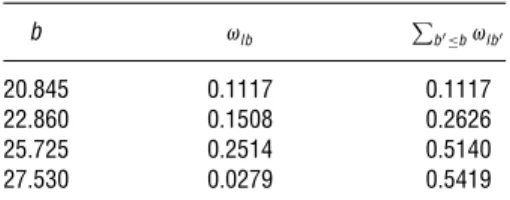
This stepwise function is useful because it approxi-mates the most adequate mapping to be applied to predictor variablelto optimize the classification task. As an illustration, Table 3 shows, for predictor vari-able Worst Texture, its cutoffs b, the corresponding weights lb, and the cumulative weightsb≤blb.
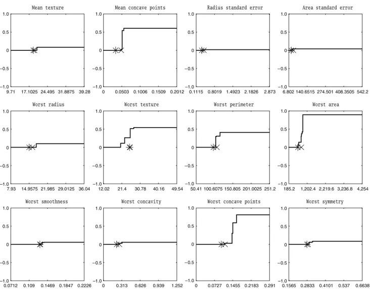
We propose a plot of function (4) to gain insight about the contribution of predictor variable l to the classifier. This plot is a valuable tool to practitioners who can use it to interpret the classifier and describe the role every predictor variable plays in the classi-fication. In particular, it allows a direct choice of the relevant predictor variables and detection of critical values and intervals.
In Figure 1, we show for each of the 12 relevant pre-dictor variables, i.e., those with at least one nonzero
Table 2 Cutoffs and Weights for Predictor VariableWorst Radius
b lb
17.720 0.1006
Table 3 Weights and Cumulative Weights for Predictor VariableWorst Texture
b lb b≤blb
20.845 0.1117 0.1117
22.860 0.1508 0.2626
25.725 0.2514 0.5140
27.530 0.0279 0.5419
lb, its contribution to the score function. Predictor
variablesMean Concave Points,Worst Area, andWorst Concave Pointsare the most important, whereasWorst Textureand Worst Perimeterhave a medium impor-tance. Using this graphical representation, in predictor variableMean Concave Points, we can detect a critical value that, as said in the previous section, is at point 0.0514. In the case of Worst Texture, in the interval between 21 and 27, the importance of this predictor variable grows up little by little, whereas outside this interval it remains constant. We can say that in this case we have a critical interval instead of a critical cutoff.
We have also plotted the median (represented by a star) and the mean (represented by a cross) in Fig-ure 1. It can be seen how, although the mean or the median are sometimes good choices for cutoffs, this does not happen in general, and BSVM prefers other choices.
Graphical representations such as Figure 1 can pro-vide insight into the role a predictor variable plays in the classifier.
In Figure 2, we present three different scenarios found by applying the proposed method to other pub-licly available databases. More details can be found in §4. In the first case, there is just one value that is critical for classification. The second instance sug-gests an S-shaped transformation, similar to Worst Texture in Figure 1; it identifies a critical interval within which the behavior is linear. Other types of mappings, harder to interpret, are possible, of course. This is the case of the third function, which suggests a logarithmic transformation.
Summing up, we have proposed a classifier that, using simple queries of type (1), allows us to visualize the role every predictor variable plays in the classifi-cation. Now it is time to describe the procedure for finding the weights lb associated to each predictor
variable and cutoff. We follow an SVM-based frame-work, developed in the next section.
2.3. Support Vector Machines
To choose and , we follow an SVM-based
approach, which consists of finding the separating hyperplane that maximizes the margin in the feature space, i.e., the space of the imagesxuof the objects u in the training sample I. The use of margin maxi-mization is theoretically motivated by the bounds on
9.71 17.1025 24.495 31.8875 39.28 –1.0 – 0.5 0 0.5 1.0 –1.0 – 0.5 0 0.5 1.0 –1.0 – 0.5 0 0.5 1.0 –1.0 – 0.5 0 0.5 1.0 –1.0 – 0.5 0 0.5 1.0 –1.0 – 0.5 0 0.5 1.0 –1.0 – 0.5 0 0.5 1.0 –1.0 – 0.5 0 0.5 1.0 –1.0 – 0.5 0 0.5 1.0 –1.0 – 0.5 0 0.5 1.0 –1.0 – 0.5 0 0.5 1.0 –1.0 – 0.5 0 0.5 1.0 Mean texture 0 0.0503 0.1006 0.1509 0.2012
Mean concave points
0.1115 0.8019 1.4923 2.1826 2.873
Radius standard error
6.802 140.6515 274.501 408.3505 542.2
Area standard error
7.93 14.9575 21.985 29.0125 36.04 Worst radius 12.02 21.4 30.78 40.16 49.54 Worst texture 50.41 100.6075 150.805 201.0025 251.2 Worst perimeter 185.2 1,202.4 2,219.6 3,236.8 4,254 Worst area 0.0712 0.109 0.1469 0.1847 0.2226 Worst smoothness 0 0.313 0.626 0.939 1.252 Worst concavity 0 0.0727 0.1455 0.2183 0.291
Worst concave points
0.1565 0.2833 0.4101 0.537 0.6638
Worst symmetry
Figure 1 Contribution of Predictor Variables
the generalization ability (Shawe-Taylor et al. 1998; Vapnik 1995, 1998), where the probability of misclassi-fying a forthcoming individual is bounded by a func-tion that is decreasing in the margin. The so-called hard marginSVM approach proposes the choice of the separating hyperplane with maximal margin, i.e., the hyperplane that correctly classifies all objects inI and
0 1 2 3 –1.0 – 0.5 0 0.5 1.0 0 50 100 150 –1 0 1 2 3 50 100 150 200 –1 0 1 2 3 4 250
Figure 2 Transformations Suggested by the Method
is farthest from the closest object. In contrast, the so-called soft margin approach allows some objects to be misclassified. We use this latter version as it has been empirically shown to avoid overfitting, a phe-nomenon that happens when a low misclassification rate in I does not generalize to forthcoming objects. The soft margin maximization problem is formulated
in this paper by min +C u∈I u s.t. cuxu++u≥1 ∀u∈I u≥0 ∀u∈I ∈N ∈ (5)
where the decision variables are the weight vector , the threshold value, and perturbationsuassociated
with the misclassification of object u∈I. · denotes the L1 norm,C is a constant that trades off the mar-gin in the correctly classified objects and the pertur-bationsu, andN=p
l=1Bl, whereSdenotes the
cardinality of a set S.
An appropriate value of C is chosen here, as detailed in §4.1, by inspecting a wide range of val-ues and then measuring the performance with respect to misclassification rates, assessed by cross-validation (Kohavi 1995).
SVM seeks the separating hyperplane maximizing a function of the distances. There are many differ-ent possible choices for the distance function, which lead to different variants of SVM (Carrizosa 2008). The distance between points has usually been consid-ered in the literature as the Euclidean norm, yield-ing the margin to be measured by the Euclidean norm as well, but other norms such as the L1 norm and theL norm have been considered and
success-fully applied. See, for instance, Bennett (1999), Bradley and Mangasarian (1998), Carrizosa et al. (2008), Mangasarian (2000, 1965), Smola et al. (1998), Weston et al. (1999), and the references therein. Moreover, the choice of the L norm to measure distances yields the minimization of the L1 norm of . In this sense, the problem is equivalent to the use of the L1 norm regularization, also called lasso penalty (Hastie et al. 2001, Tibshirani 1996).
Contrary to the Euclidean case, in which a max-imal margin hyperplane can be found by solving a quadratic program with linear constraints if, as in this paper, the L1 norm regularization is used, then an optimal solution of the corresponding optimization problem can be found by solving a linear program-ming (LP) problem. In Pedroso and Murata (2001), empirical results show that “in terms of separation performance,L1,L, and Euclidean norm-based SVM
tend to be quite similar.” Moreover, the L1 norm regularization contributes to sparsity in the classi-fier, yieldingwith many components equal to zero; see, for instance, Bradley and Mangasarian (1998), Fung and Mangasarian (2004), or Mangasarian and Thompson (2006, p. 315) which states that “one of the principal advantages of 1-norm support vector machines (SVMs) is that, unlike conventional 2-norm SVMs, they are very effective in reducing input space features for linear kernels.”
Because·is the L1 norm, problem (5) can be for-mulated as the following LP problem:
min p l=1 b∈Bl + lb+−lb+C u∈I u s.t. p l=1 b∈Bl + lb−−lbculbxu +cu+u≥1 ∀ u∈I + lb≥0 ∀b∈Bl ∀l=12 p − lb≥0 ∀b∈Bl ∀l=12 p u≥0 ∀u∈I ∈ (6)
After finding the maximal margin hyperplane in the feature space defined by, the score function has the form described in (3).
As said before, for each feature, the absolute value of its coefficient indicates the importance of that fea-ture for the classification. In particular, feafea-tures whose corresponding coefficient is zero can be seen as irrel-evant for classification purposes. Using basic linear programming theory, it is easy to see that the num-ber of features with a nonzero coefficient is not larger than the number of objects in the training sample.
3. Column Generation
Problem (6) is a large-scale linear program, which may be solved by any method that can handle SVM with the L1 norm regularization, including general-purpose LP procedures or more ad hoc methods; see, e.g., Fung and Mangasarian (2004). In this paper, we propose problem (6) to be solved by the well-known mathematical programming tool called column generation, initially introduced for the cutting-stock problem (Gilmore and Gomory 1961) and success-fully used, under different variants, in different works on support vector machines such as Bi et al. (2004), Bradley and Mangasarian (2000), Demiriz et al. (2002), and Mangasarian and Thompson (2006). A brief dis-cussion on how column generation is tailored to solve problem (6) follows.
Instead of solving problem (6) directly, which has a high number of decision variables, the column gener-ation technique solves a series of reduced problems, where decision variables corresponding to features in the set are iteratively added as needed.
For F ⊂, letmaster problem (6-F) be problem (6) with the family of featuresF. In each iteration, we first solve problem (6-F). The next step is to check whether the current solution is optimal for problem (6) or not and, in the latter case, generate a new feature , improving the objective value of the current solu-tion. The generated feature is added to the family of
featuresF. This process is repeated until optimality is reached.
To generate new features, we use the dual formu-lation of problem (6), max u∈I !u s.t. −1≤ u∈I !ucuxu≤1 ∀∈ u∈I !ucu=0 0≤!u≤C u∈I (7)
The dual formulation of the master problem (6-F) only differs from this one in the first set of constraints, which should be attained∀∈F instead of∀∈.
Let ∗ ∗ be an optimal solution of master
problem (6-F), and let !∗
uu∈I be the values of the
corresponding optimal dual solution. If the optimal solution of the master problem (6-F) is also optimal for problem (6), then for every feature∈ the con-straints of the dual problem (7) will hold; i.e.,
−1≤ u∈I !∗ ucuxu≤1 (8) Denote "=u∈I!∗ ucuxu. If ∗ ∗ is not
opti-mal for problem (6), then the most violated constraint gives us information about which feature is promis-ing and could be added toF, in the sense that adding such a feature to the set F would yield, at that iter-ation, the highest improvement of the objective func-tion. Thus, we wish to generate a new feature∈, maximizing".
In the remainder of this section, we give a more detailed description of our implementation of the col-umn generation algorithm.
3.1. Initial Set of Features
In the column generation procedure, new features are sequentially added to the problem based on the dual values of the current solution. The column generation technique starts with an initial master problem, i.e., a set of features F0 must be chosen to initialize the algorithm. We have chosen to start with one feature per predictor variable, with the cutoff set equal to its median in the objects ofI.
3.2. Generation of Features
Finding the best ∈ reduces to finding a predic-tor variable l and a cutoff b∈Bl such that "lb,
with lb defined by (2), is maximal. This can be done
by full inspection of the setlb+
l lb−l l=12 p ,
where, for each predictor variable l, the cutoff b+ l
(respectively,b−
l ) is the value inBl for which"lbis
highest (respectively, lowest). In this section, we focus
on a given predictor variable land describe an algo-rithm for finding the cutoff b+
l , maximizing "lb.
Findingb−
l can be done in a similar way.
First, we sort all the objects in decreasing order by the values of the predictor variable l. Denote by ui
the object in ith position. For simplicity, suppose there are not repeated values; i.e., xlu1> xul 2>· · ·> xuIl . The case with repeated values will be analyzed later.
Once l is fixed and all the objects are sorted by the values of the predictor variablel, the value"lb
can be efficiently calculated with a recursive proce-dure. Indeed, for certain i∈12 I , we have
"lbi+1="lbi+!∗
ui+1cui+1, where bi denotes the
cutoff chosen as xui+xui+1/2. Moreover, since !∗ u
is nonnegative for all u∈I, we have that "lbi+1≥
"lbi whenevercui+1=1. Hence, checking whether
lbi is a maximum is not needed for every ibut only
for thoseisuch thatcui=1 andcui+1= −1.
In the case in which there are repeated values in
xu
l u∈I , the rule above does not apply. Letiand t
be such that xlui−1> xlui =xlui+1 = · · · =xuil +t > xuil +t+1. Note that in the set of objects where predictor variable l has the same value, there could be objects belonging to different classes. In this case, the value
b=bimust be checked, whatever the value ofcui+t+1.
However, ifcui=cui+1= · · · =cui+tandcui+t+1=1,
we know that settingb=bjfor anyj=i i+1 i+t
will be improved by settingb=bi+t+1. This means that
b=bi does not give a maximum of "lb. Only if cui=1 andcui+t+1= −1 is it worth consideringb=b
i
as a candidate to be the maximum.
The minimization of " is done analogously. For example, in case of no repeated values, candidates to be a minimum correspond to objects ui belonging to class−1, where the next objectui+1 belongs to class 1.
Taking into account all these considerations, we obtain, for a fixed predictor variable l given the dual values!∗
u, the algorithm described below, which
finds the cutoff b+
l (and, respectively, bl−) for which "lb+
l (respectively,"lb−l) is maximal (respectively,
minimal).
Algorithm 1(Choosing two cutoffs forxl)
Step0. Sort the objects decreasingly byxl xuil .
Step1. Seti←1,sum←0,max←0,min←0,i+←i,
andi−←i.
Step2. Setsum←sum+!∗ uicui.
Step3.
Step3.1. Ifxlui=xuil +1, then, go to Step 4. Step3.2. Otherwise, if for some t >0, xui−t−1
l < xuil −t= · · · =xuil < xlui−1 and there exists j with j=
1 t and cui=cui−j, then:
• Ifsum>max, then setmax←sumandi+←i.
Step3.3. Otherwise,
• if cui=1, cui+1= −1 and sum>max, then
set max← sumandi+←i.
• if cui= −1, cui+1=1 and sum<min, then
set min←sumandi−←i.
Step4. Set i←i+1. If i≤I, then go to Step 2. Otherwise, STOP:b+
l =bi+ and b−l =bi−.
We may notice that Step 0 can be performed in a preprocessing stage of running timeOIlogIfor all calls to Algorithm 1 for predictor variablel. Hence, considering such sorting as preprocessing, it follows that each call to Algorithm 1 runs in OI time because Step 3 is performed at most once for each object in the training sample, and the calculations there involving Step 0 can be performed in constant time.
3.3. Implementation Details
The column generation algorithm has been imple-mented as follows. The initial set of featuresF0is built, as described in §3.1, using features whose cutoffs are the medians of the predictor variables. Then, prob-lem (6-F0) is solved for such initial set of features. The dual values of the optimal solution found are used to generate new features.
In every step of the column generation algorithm, instead of generating just one feature (the one max-imizing ", we generate two features for every predictor variable l, given by the cutoffs b+
l , bl− for
which "lb is, respectively, maximal and minimal.
This is done using Algorithm 1 as described in §3.2. We do it for all the predictor variables, thus obtain-ing 2p features. Those generated features having
">1 are added to F, and the LP problem (6-F) is solved. These steps are repeated until all the gener-ated features have " ≤1, in which case we have found an optimal solution of problem (6). A summary of this column generation algorithm is presented next.
Algorithm 2(Column generation) Step0. SetF0←1b∗
1 2b∗2 pb∗p , whereb
∗ l is the
median of the predictor variable l, for l=12 p. SetF ←F0.
Step1. Solve problem (6-F). Let∗ ∗be its
opti-mal solution, with dual values!∗
u∀u∈I.
Step2. For eachl=12 pdo:
Step2.1. Run Algorithm 1 to chooseb+
l andbl−.
Step2.2. If"lb+
l >1, then setF ←F ∪lb+l .
Step2.3. If"lb−
l <−1, then setF ←F ∪lbl− .
Step3. If F has been modified, then go to Step 1, otherwise STOP: we have found an optimal solution of problem (6).
In Step 1, we need to solve the LP problem (6-F). In our numerical results, we have used CPLEX 8.1.0 as the LP solver.
Our numerical experience shows that the num-ber of features used by our classifier, i.e., the ones
that have been generated by the BSVM and have a nonzero coefficient in the classifier, is usually rather large. To obtain a more simple classifier, we proceed with a wrapper feature selection procedure in which features are recursively deleted. In this procedure, which has been successfully applied in standard SVM (see Guyon et al. 2002), all the generated features with zero coefficient in the classifier as well as the feature with nonzero coefficient having the smallest absolute value are eliminated. Then, the coefficients are recom-puted by the optimization of the problem (6). This elimination procedure is repeated until the number of features with a nonzero coefficient is below a number given in advance.
This wrapper procedure is applied only in §4.5, where numerical results show that it allows one to reduce the number of features used in the classifier at the expense of a mild loss in the classification ability.
4. Numerical Results
4.1. Databases, Benchmarking Methods, and Accuracy Measure
In this section, we illustrate the classification ability as well as the most desirable properties of BSVM. With this aim, a series of numerical experiments has been performed using databases publicly available from the UCI Machine Learning Repository (Newman et al. 1998). Nine different databases were used, namely, the Sonar Database, called here sonar; the Cylinder Bands Database, called herebands; the Credit Screen-ing Database, called here credit; the Ionosphere Database, called here ionosphere; the New Diag-nostic Database, contained in the Wisconsin Breast Cancer Databases, called here wdbc; the Cleveland Clinic Foundation Database, called here cleveland; the Boston Housing Database, called herehousing; the Pima Indians Diabetes Database, called herepima; and the BUPA Liver-disorders Database, called herebupa. Where there are missing values, which occurs, for instance, inbandsandcredit, the objects with missing values were removed from the database. In databases such asbandsandcredit, some of the predictor vari-ables were nominal. Each of these predictor varivari-ables has been replaced by a set of binary variables in the following way: For every possible valuexˆof the origi-nal nomiorigi-nal predictor variablel, a new binary variable is built taking value one whenxlis equal toxˆand zero
otherwise. Thehousingdatabase is a typical regression data set, but it is often used as a classification data set where the class indicates whether the median value of houses exceeds $21,000. Finally, for each database, the final number of objects and the number of predictor variables (all quantitative) can be found in the second column of each table.
All databases used are of small to moderate size. Very large data sets do not seem to be so suitable for a crude implementation of BSVM because column generation methods are known to be time-consuming. In practice, for databases of much larger size than those used in these experiments, it might be conve-nient to either select a subsample of data with manage-able size or perform some dimensionality reduction technique such as principal component analysis to obtain an appropriate number of variables.
To compare the BSVM classifier with other classi-fiers, we have tested the performance of three differ-ent benchmarking methods: classification trees, both with pruning (TreePr) and without pruning (TreeCr); linear SVM; and a benchmarking method for the SVM with the L1 norm regularization, namely, the NLPSVM proposed in Fung and Mangasarian (2004). The classification accuracy of each method is mea-sured by the “leave-one-out correctness,” as done in Fung and Mangasarian (2004). Below, we give a brief description of this measure.
In the leave-one-out correctness, hereafter referred to aslooc,for each object, the training sample is equal to the whole database except for this object, while the testing sample is equal to the excluded object. For each training sample, we construct a classifier that will be applied in the corresponding testing sample, returning a one if the only object in the testing sample is correctly classified and zero otherwise. The looc is equal to the percentage of correctly classified objects. Because looc uses all but one object to build the clas-sifier, the provided classification can be expected to be close to the one of the classifier trained with the complete data set.
Given a training sample, it remains to specify the way the SVM as well as the BSVM classifiers are con-structed. Problem (6), as well as the corresponding optimization problem for the linear SVM, contains a parameter that needs to be tuned, namely, the regular-ization parameterC, which trades off misclassification errors in the training sample with the generalization error. As in Fung and Mangasarian (2004), we limit the values of this parameter to the values 2i withi=
−12−11 12. ParameterCis then chosen so that it minimizes the misclassification rate after performing 10-fold cross-validation in the training data (which, as said before, contains all but one object). It has been empirically observed (e.g., Bradley and Mangasarian 1998, Colas et al. 2007, Fung and Mangasarian 2004) that the choice of the parameterCmay strongly influ-ence the number of features selected. Hinflu-ence, one might have also chosenC by balancing misclassifica-tion rates and number of features selected.
4.2. Classification Ability
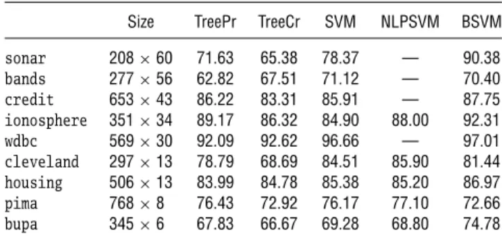
In Table 4, we report the looc of both classification trees, with and without pruning, linear SVM with
Table 4 Looc for BSVM and Benchmarking Methods
Size TreePr TreeCr SVM NLPSVM BSVM
sonar 208×60 71.63 65.38 78.37 — 90.38 bands 277×56 62.82 67.51 71.12 — 70.40 credit 653×43 86.22 83.31 85.91 — 87.75 ionosphere 351×34 89.17 86.32 84.90 88.00 92.31 wdbc 569×30 92.09 92.62 96.66 — 97.01 cleveland 297×13 78.79 68.69 84.51 85.90 81.44 housing 506×13 83.99 84.78 85.38 85.20 86.97 pima 768×8 76.43 72.92 76.17 77.10 72.66 bupa 345×6 67.83 66.67 69.28 68.80 74.78
normalized data, NLPSVM, and BSVM. Note that for NLPSVM, we only have results on five databases— the ones reported by Fung and Mangasarian (2004) in their paper. From Table 4, we can see that BSVM outperforms the three benchmarking methods in six out of the nine databases we consider in this paper. This happens in the ionosphere, the housing, and the bupa databases. For the sonar, credit, and wdbc databases, Fung and Mangasarian (2004) do not report any results, but BSVM outperforms classification trees and linear SVM. In these six databases, the increase in accuracy of BSVM with respect to the best-reported accuracy ranges from 0.35% for the wdbc database up to 12.01% for the sonar database. For the bands database, we are able to outperform classification trees but not the linear SVM, which has an accuracy of 71.12%, whereas we have 70.40%. Similarly, for the cleveland database, we are able to outperform clas-sification trees, but linear SVM and NLPSVM have a better classification accuracy, 84.51% and 85.90%, respectively. That of BSVM is 81.44%. For the pima database, BSVM underperforms the rest of the meth-ods; the decrease in accuracy of BSVM with respect to the best-reported accuracy is equal to 4.44%. As a sum-mary, we conclude that BSVM can be seen as a CART-like method (which may be very good for practitioners because relevant predictor variables and critical val-ues of them are identified) with a classification power that is at least comparable to (and in some cases much better than) competing benchmarking techniques such as CART or other versions of SVM.
4.3. Interpretability
Classification trees are widely used in applied fields as diverse as medicine (diagnosis), computer science (data structures), botany (classification), and psychol-ogy (decision theory), mainly because they are easy to interpret. Therefore, high accuracy is not the only desirable property of a classifier but also its inter-pretability. BSVM improves largely the interpretabil-ity of standard SVMs by the use of queries of type (1). In this section, we illustrate how our method takes us one step further toward interpretability via the use of the visualization tool proposed in §2.2.
70 80 90 100 – 4 – 2 0 2 4 40 60 80 100 120 – 4 – 2 0 2 4 50 100 150 – 4 – 2 0 2 4 20 40 60 80 – 4 – 2 0 2 4 50 100 150 200 250 – 4 – 2 0 2 4 0 5 10 15 20 – 4 – 2 0 2 4
Var. 1 Var. 2 Var. 3
Var. 4 Var. 5 Var. 6
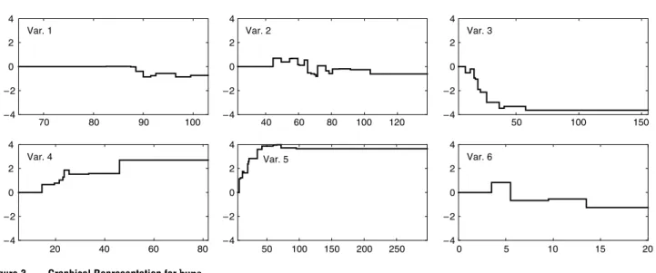
Figure 3 Graphical Representation forbupa
To do this, we have considered two databases with different characteristics, namely,bupaandsonar, which have, respectively, 6 and 60 predictor variables. Because the focus here is on interpretability and not generalization ability, the whole database has been used to build the classifier. ParameterChas been cho-sen by 10-fold cross-validation in the whole database. If SVM is performed, bupa uses all six predictor variables; i.e., all predictor variables have an asso-ciated nonzero weight. BSVM uses all six predictor variables as well; we say that a predictor variable has been used if there exists at least one feature associated to this predictor variable that has a nonzero coefficient in the classifier. The total number of features used by BSVM is 62.
A quick look at Figure 3, with information from bupa, allows us to say that predictor variables 3, 4, and 5 have the strongest influence in the classifier. It is particularly simple to analyze from the picture the influence of predictor variable 3. Indeed, we can see that predictor variable 3 presents an S-shaped form, displaying linear behavior within the interval with endpoints 0 and 25 and constant outside. Moreover, the slopes are negative, meaning that the higher the value of the predictor variable (up to 25), the stronger the tendency to be classified in the negative class. On top of that, we see that whether predictor vari-able 3 takes a value of, say, 25 or, instead, a much higher value turns out to be irrelevant for classifica-tion purposes.
A similar behavior is detected for predictor vari-able 4. From 0 to 25, the influence is linear, but after that it is stable and finally jumps around value 45. Now the slopes are positive, implying that the higher the value of predictor variable 4, the stronger the ten-dency to be classified in the positive class.
Predictor variable 5 shows a logarithmic behavior, again with positive slopes and one critical value after which the function remains almost constant.
In general, this example shows that the presence of many cutoffs, as in predictor variables 3, 4, and 5, is not an inconvenience for interpreting the classifier, whose behavior is easily detected via the visualization tool proposed.
Now, take the example of databasesonar, which has 60 predictor variables. If SVM is performed, all 60 are used again, whereas BSVM uses 98 features, involving 45 different predictor variables. Hence, BSVM is able to make feature selection (it is able to detect as irrel-evant for classification 25% of the predictor variables) in a database where linear SVM would consider all variables as relevant.
In Figure 4, the 45 used predictor variables are shown, renumbered for convenience. A simple look to this figure indicates that there are only 4 out of the 45 predictor variables with strong influence in the clas-sifier, namely, predictor variables 11, 20, 26, and 36. Predictor variables in positions 11 and 20 have just one main critical value, whereas predictor variables 26 and 36 present an almost linear behavior in a clearly iden-tified interval.
We see again that the use of BSVM allows us to choose the relevant predictor variables, interpret the way such variables influence the classifier, and detect the critical values and intervals for each predictor variable.
4.4. Size of the BSVM Classifier
Simplicity in the classifier is another desirable prop-erty for practitioners. Because both BSVM and classi-fication trees are based on simple queries of type (1), the size of the resulting classifier is a good proxy for their complexity.
In Table 5, we compare the size of the classifiers constructed by BSVM and classification trees. We report average results over all the objects, i.e., over all the testing samples.
0.06 0.13 –1 0 1 –1 0 1 –1 0 1 –1 0 1 –1 0 1 –1 0 1 –1 0 1 –1 0 1 –1 0 1 –1 0 1 –1 0 1 –1 0 1 –1 0 1 –1 0 1 –1 0 1 –1 0 1 –1 0 1 –1 0 1 –1 0 1 –1 0 1 –1 0 1 –1 0 1 –1 0 1 –1 0 1 –1 0 1 –1 0 1 –1 0 1 –1 0 1 –1 0 1 –1 0 1 –1 0 1 –1 0 1 –1 0 1 –1 0 1 –1 0 1 –1 0 1 –1 0 1 –1 0 1 –1 0 1 –1 0 1 –1 0 1 –1 0 1 –1 0 1 –1 0 1 –1 0 1
Var. 1 Var. 2 Var. 3 Var. 4 Var. 5 Var. 6 Var. 7
Var. 8 Var. 9 Var. 10 Var. 11 Var. 12 Var. 13 Var. 14
Var. 15 Var. 16 Var. 17 Var. 18 Var. 19 Var. 20 Var. 21
Var. 22 Var. 23 Var. 24 Var. 25 Var. 26 Var. 27 Var. 28
Var. 29 Var. 30 Var. 31 Var. 32 Var. 33 Var. 34 Var. 35
Var. 36 Var. 37 Var. 38 Var. 39 Var. 40 Var. 41 Var. 42
Var. 43 Var. 44 Var. 45
0.11 0.23 0.15 0.30 0.21 0.42 0.20 0.40 0.18 0.37 0.23 0.45 0.34 0.68 0.36 0.71 0.38 0.36 0.70 0.36 0.71 0.51 0.50 1.00 0.50 0.99 0.51 1.00 0.52 1.00 0.52 1.00 0.51 1.00 0.52 1.00 0.54 1.00 0.52 1.00 0.51 1.00 0.50 1.00 0.53 1.00 0.50 0.96 0.48 0.93 0.52 1.00 0.50 1.00 0.49 0.94 0.51 1.00 0.51 0.98 0.47 0.92 0.41 0.82 0 0.38 0.77 0 0.35 0.70 0 0.36 0.72 0 0.16 0.33 0 0.05 0.10 0.03 0.07 0.03 0.02 0.04 0.02 0.04 0.01 0.03 0.02 0.04 0.73 0.99 0.01
Figure 4 Graphical Representation forsonar
For both classification trees, with and without prun-ing, we report the total number of nodes in the final tree as well as the number of leaf nodes. For the BSVM classifier, we report the number of used predic-tor variables as well as the number of used features.
In our opinion, the fairest comparison for the com-plexity is to measure the number of nodes generated by classification trees against the number of features
Table 5 Size of Benchmarking Classifiers
TreePr TreeCr BSVM
leaf TreePr leaf TreeCr predictor BSVM
Size nodes nodes nodes nodes variables features
sonar 208×60 2.76 452 18.40 3580 4510 97.50 bands 277×56 8.95 1691 28.81 5662 2340 78.80 credit 653×43 2.11 321 42.71 8442 1850 80.00 ionosphere 351×34 3.00 500 18.94 3688 2720 71.60 wdbc 569×30 5.45 990 16.00 3100 2600 74.20 cleveland 297×13 5.33 967 23.00 4501 1220 32.00 housing 506×13 4.58 816 33.84 6667 1200 68.30 pima 768×8 4.06 711 69.15 13729 800 61.50 bupa 345×6 3.76 652 36.99 7299 600 43.90
used by BSVM. As the results show, the size of the classification tree with pruning is always smaller. For the classification tree without pruning, in four out of the nine databases, namely, credit, cleveland, pima, andbupa, BSVM is smaller in size. In a fifth database, housing, both classifiers are of similar size. The result-ing complexity for BSVM should be balanced with its better classification ability. From Table 4, BSVM outperforms classification trees with pruning except for the pima database, with an increase in accuracy that ranges from 1.53% for thecreditdatabase up to 18.75% for the sonar database. Similarly, BSVM out-performs classification trees without pruning except for the pima database in which both methods have basically the same accuracy. The increase in accuracy of BSVM ranges from 2.19% for thehousingdatabase up to 25.00% for thesonardatabase.
From the numerical experience reported, we can assert that BSVM outperforms classification trees in terms of its classification ability at the expense of a higher complexity of the classifier, which is compara-ble to the complexity of classification trees if no prun-ing is performed.
Table 6 Looc of BSVM After Reducing the Number of Features to a Maximum of 30
Best(BSVM+ # of features
Size reported BSVM wrapper) in BSVM
sonar 208×60 78.37 90.38 87.50 97.50
ionosphere 351×34 89.17 92.31 92.02 71.60
cleveland 297×13 85.90 81.44 81.48 32.00
housing 506×13 85.38 86.97 86.76 68.30
bupa 345×6 69.28 74.78 73.04 43.90
4.5. Reducing the Number of Used Features
The complexity of the classifiers obtained by BSVM is usually high because a high number of features may be present in the rule, as we have discussed in the previous section. With the aim of reducing the com-plexity of the classifier obtained by our procedure, we have performed several experiments implement-ing the wrappimplement-ing procedure described in §3.3. Due to computational burden, we present results on five databases. The selection of the databases has been done based on the running times, and it does not affect our conclusions. In Table 6, results on databasessonar, ionosphere,cleveland,housing, andbupaare shown. For convenience, we repeat some of the results already given in previous tables. The third and fourth columns of Table 6 report the best accuracy among all three benchmarking methods as well as the one of BSVM (when no wrapper procedure is applied), both processed from the data in Table 4. The fifth column reports the accuracy of BSVM when the size of the classifier is reduced up to a maximum of 30 features. The sixth column contains the size (mea-sured as number of used features) of the BSVM clas-sifier, obtained from Table 5. From those results, we can conclude that the classification ability of BSVM slightly deteriorates. More specifically, the cleveland database, which was one in which the linear SVM outperformed BSVM, has essentially the same accu-racy as before. This is not surprising because the aver-age number of features used by BSVM is equal to 32, as reported in Table 5. For the ionosphere and the housing databases, the looc remains almost the same and, therefore, BSVM outperforms the best of the three benchmarking methods while using at most 30 features. In thebupadatabase, the decrease in accu-racy is equal to 1.74%, but even after this deteri-oration, BSVM with wrapping procedure still gives us the best accuracy. The conclusions for the sonar database are similar. Thus, even with this limit on the number of features, BSVM is still able to outperform the three benchmarking methods except for the case of theclevelanddatabase in which, as happens with-out wrapping, BSVM is with-outperformed by the linear SVM and the NLPSVM.
We decided to further investigate those databases in which the wrapping of the BSVM classifiers did not
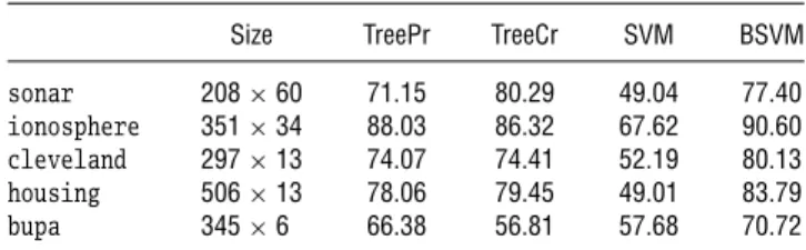
Table 7 Looc for BSVM and Benchmarking Methods in Databases with Outliers
Size TreePr TreeCr SVM BSVM
sonar 208×60 71.15 80.29 49.04 77.40
ionosphere 351×34 88.03 86.32 67.62 90.60
cleveland 297×13 74.07 74.41 52.19 80.13
housing 506×13 78.06 79.45 49.01 83.79
bupa 345×6 66.38 56.81 57.68 70.72
affect the accuracy, namely, thecleveland,ionosphere, and housing databases. In the housing database, the wrapped BSVM classifier, as said above, has the best accuracy although its size is half of that from the tree without pruning (which is the best of the two trees in terms of accuracy). Forclevelandandionosphere, the size was not competitive enough. Therefore, we fur-ther reduced the number of used features to a maxi-mum of 20. The looc ofclevelandandionospherewas exactly the same as the one obtained when the number of used features was limited to 30. This is especially remarkable for theionospheredatabase, in which we can reduce the number of features to less than a third, from 7160 to at most 20, while the accuracy decreases only by 0.29%.
4.6. Presence of Outliers
The classifier proposed in this paper is based on threshold functions; thus, it seems that extreme obser-vations, with very high or very low values, will not have a strong influence in the classifier. To empirically test this conjecture, a series of experiments has been performed where some outliers were artificially intro-duced. Every cell in the database was chosen to be an outlier with probability 0.05. Those cells chosen were modified by adding ( times the range of its predic-tor variable in the training sample. We present here results for(=10. For other values of(, we obtained similar results and, therefore, do not report them here. As in §4.5 and again due to computational bur-den, we present results on five databases. In Table 7, results on databases sonar, ionosphere, cleveland, housing, and bupa are shown. We compare BSVM against classification trees and linear SVM. We do not report results on the NLPSVM because outliers are not discussed in the paper of Fung and Mangasar-ian (2004). The classification ability of the linear SVM classifier dramatically worsens when introducing out-liers and clearly underperforms the other two meth-ods. Classification trees and BSVM are only slightly affected. We outperform classification trees in all databases except sonar. Therefore, our conjecture is supported.
5. Conclusions and Further Research
In this paper, a new SVM-based tool for supervised classification has been proposed. The classifier gives
insightful knowledge about the way the predictor variables influence the classification. Indeed, the non-linear behavior of the data is modeled by the BSVM classifier using simple queries of type (1), easily inter-pretable by practitioners.
In terms of generalization ability, BSVM is com-petitive against classification trees and SVM because it has a higher leave-one-out correctness in most databases tested. Moreover, by its nature, BSVM is an interesting tool when a good classification abil-ity is required, but interpretabilabil-ity of the results is also important. Indeed, even though the crude BSVM may yield a large set of features with nonzero coeffi-cients, we have shown that interpretability might also be possible in this situation: we can use a graphical method for getting insight about the role each predic-tor variable plays in the classifier. If needed, a wrap-ping procedure enables one to keep the number of features used at a desired level at the expense of a slight deterioration in the classification ability.
Concerning robustness, some numerical tests have been performed to analyze how the classification abil-ity (slightly) deteriorates when outliers exist. We can conclude from the results that BSVM is much more robust than linear SVM against outliers.
Several issues analyzed in this paper may deserve further study. For instance, the sets Bl contain, by definition, all midpoints among consecutive values of each predictor variable in the training sample. An adequate filtering in a preprocessing step would reduce the computational burden, especially for large data sets, and might help to reduce the overfitting that a very complex model may produce.
The binarization procedure has been applied to each predictor variable separately. If interactions be-tween predictor variables are expected to be relevant, more general binarization procedures might be con-sidered. These issues, as well as extension to support vector regression, will be addressed in the near future.
Acknowledgments
The authors thank the two anonymous referees and the asso-ciate editor for their helpful comments to improve both the exposition as well as the numerical results in §4. The authors are grateful to Jingbo Wang and Rafael Blanquero for the support they have offered to obtain some of the results in §4. This work has been partially supported by projects MTM2005-09362-C03-01 of the Ministerio de Educación y Ciencia, Spain, and FQM-329 of Junta de Andalucía, Spain.
References
Andrews, R., J. Diederich, A. B. Tickle. 1995. A survey and critique of techniques for extracting rules from trained artificial neural networks.Knowledge Based Systems8(6) 373–389.
Baesens, B., R. Setiono, C. Mues, J. Vanthienen. 2003. Using neu-ral network rule extraction and decision tables for credit-risk evaluation.Management Sci.49(3) 312–329.
Barakat, N., J. Diederich. 2004. Learning-based rule-extraction from support vector machines.Proc. 14th Internat. Conf. Comput. The-ory Appl.ICCTA 2004,Alexandria,Egypt, http://espace.library. uq.edu.au/view.php?pid=UQ:9624.
Barakat, N., J. Diederich. 2005. Eclectic rule-extraction from support vector machines.Internat. J. Comput. Intelligence2(1) 59–62. Bennett, K. 1999. Combining support vector and mathematical
programming methods for induction. B. Schölkopf, C. Burges, A. Smola, eds.Advances in Kernel Methods: Support Vector Learn-ing. MIT Press, Cambridge, MA, 307–326.
Bi, J., T. Zhang, K. P. Bennett. 2004. Column-generation boost-ing methods for mixture of kernels.Proc. 10th ACM SIGKDD Internat. Conf. Knowledge Discovery Data Mining,Seattle, ACM, New York, 521–526.
Bradley, P. S., O. L. Mangasarian. 1998. Feature selection via con-cave minimization and support vector machines.Machine Learn-ing Proc. 15th Internat. Conf. (ICML ’98), Morgan Kaufmann, San Francisco, 82–90.
Bradley, P. S., O. L. Mangasarian. 2000. Massive data discrimination via linear support vector machines.Optim. Methods Software13 1–10.
Carrizosa, E. 2008. Support vector machines and distance mini-mization. P. M. Pardalos, P. Hansen, eds.Data Mining and Mathe-matical Programming,CRM Proc. Lecture Notes, Vol. 45. American Mathematical Society, Providence, RI, 1–14.
Carrizosa, E., B. Martín-Barragán, D. Romero Morales. 2008. Multi-group support vector machines with measurement cost: A biob-jective approach.Discrete Appl. Math.156(6) 950–966.
Colas, F., P. Paclík, J. N. Kok, P. Brazdil. 2007. Does SVM really scale up to large bag of words feature spaces? M. R. Berthold, J. Shawe-Taylor, N. Lavrac, eds.Advances in Intelligent Data Anal-ysis VII,Lecture Notes in Computer Science, Vol. 4723. Springer, Berlin, 296–307.
Cortes, C., V. Vapnik. 1995. Support-vector networks.Machine Learn. 20(3) 273–297.
Craven, M., J. Shavlik. 1997. Using neural networks for data min-ing.Future Generation Comput. Systems13(2–3) 211–229. Demiriz, A., K. P. Bennett, J. Shawe-Taylor. 2002. Linear
program-ming boosting via column generation. Machine Learn. 46(1–3) 225–254.
Fung, G., O. L. Mangasarian. 2004. A feature selection Newton method for support vector machine classification. Comput. Optim. Appl.28(2) 185–202.
Fung, G., S. Sandilya, R. Bharat Rao. 2005. Rule extraction from linear support vector machines.Proc. 11th ACM SIGKDD Inter-nat. Conf. Knowledge Discovery Data Mining,Chicago, ACM, New York, 32–40.
Gilmore, P. C., R. E. Gomory. 1961. A linear programming approach to the cutting-stock problem.Oper. Res.9(6) 849–859.
Guyon, I., J. Weston, S. Barnhill, V. Vapnik. 2002. Gene selection for cancer classification using support vector machines.Machine Learn.46(1–3) 389–422.
Hand, H., H. Mannila, P. Smyth. 2001. Principles of Data Mining. MIT Press, Cambridge, MA.
Hastie, T., R. Tibshirani. 1998. Classification by pairwise coupling. Ann. Statist.26(2) 451–471.
Hastie, T., R. Tibshirani, J. Friedman. 2001.The Elements of Statis-tical Learning: Data Mining,Inference,and Prediction. Springer, New York.
Herbrich, R. 2002.Learning Kernel Classifiers. Theory and Algorithms. MIT Press, Cambridge, MA.
Kohavi, R. 1995. A study of cross-validation and bootstrap for accu-racy estimation and model selection. Proc. 14th Internat. Joint Conf. Artificial Intelligence. Morgan Kaufmann, San Francisco, 1137–1143.
Mangasarian, O. L. 1965. Linear and nonlinear separation of pat-terns by linear programming.Oper. Res.13(3) 444–452. Mangasarian, O. L. 2000. Generalized support vector machines.
A. Smola, P. Bartlett, B. Schölkopf, D. Schuurmans, eds.Advances in Large Margin Classifiers. MIT Press, Cambridge, MA, 135–146.
Mangasarian, O. L., M. E. Thompson. 2006. Massive data classi-fication via unconstrained support vector machines. J. Optim. Theory Appl.131(3) 315–325.
Martens, D., B. Baesens, T. Van Gestel, J. Vanthienen. 2007. Com-prenhensible credit scoring models using rule extraction from support vector machines.Eur. J. Oper. Res.183(3) 1466–1476. Newman, D. J., S. Hettich, C. L. Blake, C. J. Merz. 1998. UCI
machine learning repository. Department of Information and Computer Sciences, University of California, Irvine, Irvine, http://www.ics.uci.edu/∼mlearn/MLRepository.html. Núñez, H., C. Angulo, A. Català. 2002. Rule extraction from
support vector machines. Proc. Eur. Sympos. Artificial Networks ESANN’2002,Bruges,Belgium, 107–112.
Pedroso, J. P., N. Murata. 2001. Support vector machines with differ-ent norms: Motivation, formulations and results.Pattern Recog-nition Lett.22(12) 1263–1272.
Shawe-Taylor, J., P. L. Bartlett, R. C. Williamson, M. Anthony. 1998. Structural risk minimization over data-dependent hierarchies. IEEE Trans. Inform. Theory44(5) 1926–1940.
Smola, A., T. T. Frieß, B. Schölkopf. 1998. Semiparametric support vector and linear programming machines. M. J. Kearns, S. A. Solla, D. A. Cohn, eds.Advances in Neural Information Processing Systems 11. MIT Press, Cambridge, MA, 585–591.
Tibshirani, R. 1996. Regression shrinkage and selection via the lasso.J. Royal Statist. Soc. Ser. B58(1) 267–288.
Vapnik, V. N. 1995. The Nature of Statistical Learning Theory. Springer-Verlag, New York.
Vapnik, V. N. 1998.Statistical Learning Theory. John Wiley & Sons, New York.
Weston, J., A. Gammerman, M. O. Stitson, V. Vapnik, V. Vovk, C. Watkins. 1999. Support vector density estimation. B. Schölkopf, C. Burges, A. Smola, eds.Advances in Kernel Methods—Support Vector Learning. MIT Press, Cambridge, MA, 293–305.