Algorithms for the multi-objective vehicle routing problem with hard time windows and stochastic travel time and service time

warwick.ac.uk/lib-publications

Original citation:

Miranda, Douglas M., Branke, Juergen and Conceição, Samuel V. (2018) Algorithms for the multi-objective vehicle routing problem with hard time windows and stochastic travel time and service time. Applied Soft Computing, 70 . pp. 66-79. doi:10.1016/j.asoc.2018.05.026

Permanent WRAP URL:

http://wrap.warwick.ac.uk/102771

Copyright and reuse:

The Warwick Research Archive Portal (WRAP) makes this work by researchers of the University of Warwick available open access under the following conditions. Copyright © and all moral rights to the version of the paper presented here belong to the individual author(s) and/or other copyright owners. To the extent reasonable and practicable the material made available in WRAP has been checked for eligibility before being made available.

Copies of full items can be used for personal research or study, educational, or not-for-profit purposes without prior permission or charge. Provided that the authors, title and full bibliographic details are credited, a hyperlink and/or URL is given for the original metadata page and the content is not changed in any way.

Publisher’s statement:

© 2018, Elsevier. Licensed under the Creative Commons Attribution-NonCommercial-NoDerivatives 4.0 International http://creativecommons.org/licenses/by-nc-nd/4.0/ A note on versions:

The version presented here may differ from the published version or, version of record, if you wish to cite this item you are advised to consult the publisher’s version. Please see the ‘permanent WRAP url’ above for details on accessing the published version and note that access may require a subscription.

Algorithms for the Multi-Objective Vehicle Routing Problem with Hard Time

Windows and Stochastic Travel Time and Service Time

Douglas M. Miranda

a

_{, Juergen Branke}

b_,

_{Samuel V. Conceição}

a

a_{Department of Production Engineering, Federal University of Minas Gerais, 6627, Antônio Carlos Avenue, Belo} Horizonte, Brazil

b_{Warwick Business School, The University of Warwick, Coventry CV4 7AL, UK}

E-mails:

Douglas M. Miranda [email protected] Juergen Branke [email protected] Samuel V. Conceição [email protected]

Corresponding Author:

Douglas Moura Miranda, PhD. Federal University of Minas Gerais

6627, Antônio Carlos Avenue, Belo Horizonte, Brazil Tel: (+55) 31 - 992059811

Algorithms for the Multi-Objective Vehicle Routing Problem with Hard Time

Windows and Stochastic Travel Time and Service Time

ABSTRACT

This paper introduces a multi-objective vehicle routing problem with hard time windows and stochastic travel and service times. This problem has two practical objectives: minimizing the operational costs, and maximizing the service level. These objectives are usually conflicting. Thus, we follow a multi-objective approach, aiming to compute a set of Pareto-optimal alternatives with different trade-offs for a decision maker to choose from. We propose two algorithms (a Multi-Objective Memetic Algorithm and a Multi-Objective Iterated Local Search) and compare them to an evolutionary multi-objective optimizer from the literature. We also propose a modified statistical method for the service level calculation. Experiments based on an adapted version of the 56 Solomon instances demonstrate the effectiveness of the proposed algorithms.

Keywords: vehicle routing with time windows; stochastic travel times; evolutionary and memetic

algorithms; iterated local search; multiobjective optimization.

1. Introduction

The classic vehicle routing problem with time windows (VRPTW) assumes the travel times between customers and the service times at the customers are known and deterministic. However, in real life applications, these two parameters are often stochastic, and models that takes into consideration this uncertainty can provide more accurate answers for the decision maker. Over the years, the customer expectations in the logistics sector have continuously increased and more customer-oriented business models have been demanded, for instance, ensuring a particular level of service at individual customers.

In business terms, the minimization of the operational costs of delivering the goods to the customers is a common objective. Defining service level as the probability of a vehicle visiting a customer before the end of the time window, it is plausible to say that the higher the customer service level, the higher is the customer satisfaction, motivating the inclusion of the service level as one objective function of the model.

Because operational costs and service level have very different dimensions, combining them into one single objective is not straightforward. Additionally, there seem to be a conflict between these objectives, motivating the modeling of the problem as multiobjective (MO-VRPTW). A MO-VRPTW can provide the decision maker with more comprehensive information about the problem, and once they acquire a knowledge from a set of non-dominated solutions, it is easier to define criteria to pick a single solution, by intuition or through the use of multi-criteria decision-making techniques (MCDM), e.g. Shi et al. (2009).

In this context, this paper tackles a problem considering realistic features presented in real applications such as stochastic travel time and service time, a constraint with a lower bound for the customer service level, and the consideration of two objectives (maximizing service level and minimizing operational costs).

The main contributions of this paper are:

1. The introduction of the multiobjective vehicle routing problem with hard time windows and stochastic travel and service times.

2. The design and implementation of two new algorithms (a Memetic Algorithm and Iterated Local Search) discussing specific components such as the design and utilization of the local searches, specific strategies for selection, cross-over, exit criteria and speed-up techniques. 3. An improved version of the method to calculate service levels from Miranda and Conceição

(2016) that better reflects the lower bound constraint on the distribution of travel and service times.

The problem approached in this study has hard time windows which means the vehicle has to wait in case it arrives before the start of the time window. There is a single depot, the vehicles have the same capacity and they always visit and deliver the service at the customers. The service time and the travel time are both random variables with a nonnegative normal probability distribution. Common distributions used for the travel time are normal, lognormal and Gamma distributions (Tas et al. 2013). Many studies consider the travel time normally distributed including Kenion & Morton (2003), Jie et al. (2010), Hofleitner et al. (2012), and Chen et al. (2014).

The paper is structured as follows. We give a literature review in Section 2, followed by a mathematical formulation of the problem in Section 3. Next, in Section 4, we present the developed method to calculate the service level of the customers. Section 5 explains the metaheuristics developed to solve the Multiobjective VRP with hard time windows and stochastic travel time and service time. Section 6 has experiments testing the performance of the proposed statistical method and heuristics. Finally, the main findings and conclusions are highlighted in Section 7.

2. Literature Review

Literature reviews of the Stochastic Vehicle Routing Problem (SVRP) have been provided for example by Gendreau et al. (1996, 2014) and Zeimpekis et al. (2007). Berhan et al. (2014) present a comprehensive survey on the SVRP and a classification of the papers. Most SVRP literature focuses on stochastic demand (Laporte et al., 2002 and Dror, 2016), customers’ presence (see, e.g. Gendreau et al., 1995) and both demand and presence (Balaprakash, 2015).

In the context of the VRPTW and stochastic travel times and/or service times it is important to separate the formulations without waiting time from the formulations with waiting time for the vehicles. Models without waiting time benefit from the use of convolution properties while summing the random variables. The probability distribution of the sum of two or more independent random variables is the convolution of their individual distributions and many well-known distributions have simple convolutions when there is no waiting time.

For the VRPTW with stochastic travel/service time and no propagation of the waiting time, some relevant studies were conducted by Russell & Urban (2008), Tas et al. (2013), Tas et al. (2014) and Vareias et al. (2017). In the context of VRPTW with stochastic travel/service time and with waiting time (in which the present paper is situated), studies were conducted by Jula et al. (2006), Chang et al. (2009), Li et al. (2010), Miranda (2011), Errico et al. (2013 and 2016), Zhang et al. (2013), Ehmke et al. (2015), Binart et al. (2016), Miranda and Conceição (2016) and Gutierrez et al. (2016). These studies are discussed below in more detail. Jula et al. (2006) suggest methods of estimating the mean and variance of a vehicle’s arrival time at customers using first-order approximation of Taylor series. Chang et al. (2009) studied the relationship between arrival time and time window, and developed an approach to calculate the mean and variance of the arrival time with the assumption of normality. Li et al. (2010) use Monte Carlo simulation to calculate the service level. Errico (2013) and Errico et al. (2016) propose a formulation considering a symmetric triangular distribution with an exact solution. Zhang et al. (2013) adapt the method α-discrete from Miller-Hooks & Mahmassani (1998) to estimate the arrival time distribution at a customer. The method is applied to a normal distribution and log normal distribution for the travel time, and normal distribution for the service time.

Ehmke et al. (2015) propose a method based on the application of extreme value theory that allows the computation of the distribution of the maximum of two normal variables. Even though the arrival time distribution is not normal, they assume so, and evaluate the error of this assumption in an experiment. Binart et al. (2016) solve a variant of the VRP where it’s assumed that service as well as travel times are stochastic, both with discrete triangular distributions. Miranda and Conceição (2016) introduce a method to compute the probability of the vehicle arriving before the end of a time window for the case where service time and travel time follow a Gaussian distribution. A single objective VRPTW is solved through Iterated Local Search. Finally, Gutierrez et al. (2016) develop a memetic algorithm to solve a single objective version of the VRPTW with stochastic travel and service times. The method used to compute the service level comes from Ehmke et al. (2015) and the only modification is that both travel time and service time are stochastic.

Still regarding the variant with propagation of waiting times, papers mentioned previously use triangular distributions such as Binart et al. (2016), Errico (2013) and Errico et al. (2016), which is a poor representation for real applications. Li et al. (2010) use Monte Carlo simulation (too expensive to be used in an NP-hard problem). Jula et al. (2006) use first-order approximation of Taylor series which deliver poor results. Ehmke et al. (2015) use extreme value theory but also assuming the arrival time distribution is normal. Zhang et al. (2013) does not assume the arrival time is normal even with normal travel time and service time, and its method is used as a benchmark for the statistical method of our paper.

All papers mentioned previously consider the service level as a constraint in the model and they use operational cost as single objective. Several papers propose additional objectives for the VRPTW, such as: the number of used vehicles, total traveled distance, traveling time of the longest route (makespan), total waiting time, and total delay time (Castro et al., 2011). To the best of our knowledge, no publication so far used service level.

Our paper differs from and extends the existing work in the following ways: It is the first attempt to approach a bi-objective variant of the VRPTW with stochastic travel times and service times, where the service level is one of the objectives. It proposes a new approach to embed a local search into a multi-objective problem. In addition to that, our statistical method to calculate the service level (already validated in Miranda and Conceição, 2016) has been changed to consider a more realistic representation of real problems (discussed in Section 4).

3. Background

3.1 – Multi-objective Optimization (MOO)

MOO is the process of simultaneously optimizing two or more conflicting objectives. In mathematical terms, a multiobjective optimization problem (MOP) cab be written, without loss of generality, as

𝑚𝑖𝑛 𝑓(𝑥) = (𝑓1(𝑥), 𝑓2(𝑥) , … , 𝑓𝑝(𝑥)) subject to 𝑥 ∈ 𝑋 ⊆ ℜ𝑛 where 𝑋 is a constraint set in the

multi-dimensional space of the problem specified by 𝑋 = {𝑥 ∈ ℜ𝑛_{: 𝑔} 𝑖

(𝑥) _{≤ 0, 𝑖 = 1, … , 𝑚; ℎ} 𝑗

(𝑥) _{= 0, 𝑗 = 1, … , 𝑙}.}

Given two feasible solutions 𝑥 and 𝑦, we say that 𝑥 dominates 𝑦, if ∀𝑖: 𝑓𝑖(𝑥) ≤ 𝑓𝑖(𝑦) and ∃𝑗: 𝑓𝑗(𝑥) < 𝑓𝑗(𝑦).

Moreover, 𝑥 is said to be Pareto optimal if and only if it is not dominated by any other feasible solution. The aim is to find the set of Pareto optimal solutions usually called Pareto set. This set maps to a number of non-dominated points in the objective space, the so-called Pareto Front.

Pareto ranking is often used to rank solutions: All non-dominated solutions are assigned rank 1, and inductively, all solutions non-dominated once ranks 1…i have been removed are assigned rank 𝑖 + 1.

3.2 – Problem statement

Let 𝐺 = (𝑉0, 𝐴) be a complete digraph, where 𝑉0= {0, … , 𝑛} is a set of vertices and 𝐴 = {(𝑖, 𝑗): 𝑖, 𝑗 ∈ 𝑉0, 𝑖 ≠ 𝑗} is a set of arcs. Vertex 0 represents the depot where 𝑚0 vehicles with capacity 𝑄 are

available. The set of customers is 𝑉 = 𝑉0\{0} = {1, … , 𝑛}. Each customer 𝑖 ∈ 𝑉 has a non-negative

demand 𝑞𝑖, service time 𝑆𝑇𝑖, and a time window [𝑒𝑖, 𝑙𝑖], where 𝑒𝑖 is the start of the time window (earliest time)

and 𝑙𝑖 is the end of the time window (latest time). If the vehicle arrives at customer 𝑖 before 𝑒𝑖, it is necessary

to wait until 𝑒𝑖. A travel time 𝑇𝑇𝑖𝑗 is assigned to each arc (𝑖, 𝑗) ∈ 𝐴. Both 𝑇𝑇𝑖𝑗 and 𝑆𝑇𝑖 are random variables

with known and independent probability density. 𝑆𝐿𝑖= 𝑃(𝐴𝑇𝑖≤ 𝑙𝑖) is the service level at customer 𝑖. The

vector 𝑆𝐿 = (𝑆𝐿1, … , 𝑆𝐿𝑛) summarizes the service level of each customer. Other delimitations are: 𝑄 ≥ 𝑞𝑖, 𝑖 ∈ 𝑉 (i.e., each vehicle has enough capacity to serve at least one customer) and 𝑚0∗ 𝑄 ≥ ∑𝑛𝑖=1𝑞𝑖 (i.e. the

fleet is big enough to serve all the customers). There is no time window for the depot, i.e. [𝑒0, 𝑙0] = [0, ∞].

Further notation includes:

𝑓 Fixed cost for one vehicle

𝑚 Number of vehicles in a feasible solution, 𝑚 ≤ 𝑚0 𝑐 Fixed cost for each unit of the travel time 𝑇𝑇𝑖𝑗

𝐾 Set of required vehicles in a feasible solution 𝐾 = {1, … , 𝑚}.

𝑥𝑖𝑗𝑘 Boolean variable with value 1 if vehicle 𝑘 serves arc (𝑖, 𝑗) 𝐴𝑇𝑖 Arrival time at customer 𝑖

𝑆𝑆𝑖 Service start time at customer 𝑖

𝛼𝑖 Required service level by customer 𝑖 where 𝛼𝑖 ∈ [0,1]

The decision variables of the problem are 𝑥𝑖𝑗𝑘 and 𝑚. The model for the problem can be described

as follows: 𝑀𝑖𝑛 𝑓 ∗ 𝑚 + ∑ ∑ 𝐸(𝑇𝑇𝑖𝑗) ∗ 𝑐 ∗ 𝑥𝑖𝑗𝑘 𝑘∈𝐾 (𝑖,𝑗)∈𝐴 (1) 𝑀𝑖𝑛 − 𝐸[𝑆𝐿] (2) Subject to: ∑ ∑ 𝑥𝑖𝑗𝑘 𝑘∈𝐾 𝑗∈𝑉0 = 1, ∀𝑖 ∈ 𝑉 ₍₃₎ ∑ 𝑥0𝑗𝑘 = 1, ∀𝑘 ∈ 𝐾 𝑗∈𝑉 (4) ∑ 𝑥𝑖0𝑘 = 1, ∀𝑘 ∈ 𝐾 𝑖∈𝑉 (5) ∑ 𝑥𝑖𝑗𝑘 𝑖∈𝑉0 − ∑ 𝑥𝑗𝑖𝑘 = 0, 𝑖∈𝑉0 ∀𝑗 ∈ 𝑉, 𝑘 ∈ 𝐾 ₍₆₎ ∑ 𝑞𝑖 ∑ 𝑥𝑖𝑗𝑘≤ 𝑄, ∀𝑘 ∈ 𝐾 𝑗∈𝑉₀ 𝑖∈𝑉 (7) 𝑃(𝐴𝑇𝑖 ≤ 𝑙𝑖) ≥ 𝛼𝑖, ∀𝑖 ∈ 𝑉 (8) 𝑒𝑖≤ 𝑆𝑆𝑖, ∀𝑖 ∈ 𝑉 (9)

The two objectives are given by Equations (1) and (2). Equation (1) is formed by two parts: the vehicle fixed cost (number of vehicles 𝑚 multiplied by the fixed cost 𝑓) and the variable cost (the sum of the mean of each activated arc multiplied by the cost 𝑐 per unit of travel time). Therefore, both terms are expressed by a financial unit. The second objective is given by Equation (2) and maximizes the service level of the solution, defined here as the mean of the service levels of all customers.

Equation (3) ensures each customer is visited only once. Equations (4) and (5) ensure each vehicle starts the route in the depot and also returns to it. Equation (6) ensures that each vehicle departs from a customer location after it visits the customer. Equation (7) is the capacity constraint. Equation (8) is the service level required by each customer. It reflects that the probability of a vehicle arriving at the customer before the end of the time window should be greater than a given threshold, for any customer. Equation (9) ensures the

hard time windows, where the service will only start after the start of the time window, therefore, if the vehicle arrives before 𝑒𝑖, it must wait until 𝑒𝑖. The service start time is given by Equation 10:

𝑆𝑆𝑖 = 𝑚𝑎𝑥{𝐴𝑇𝑖, 𝑒𝑖}, (10)

where 𝐴𝑇𝑖 = 𝑆𝑆𝑖−1+ 𝑆𝑇𝑖−1+ 𝑇𝑇𝑖−1,𝑖.

Note that the departure time from the depot is defined as zero and a departure time greater than zero does not improve any of the objectives.

Regarding the service level objective, we use the mean service level rather than median or percentage of customers within service level because we assume there is also a value in over-achieving the desired service level 𝛼𝑖.

4 – Computation of the service level

This section presents the statistical method to calculate the probability of a vehicle arriving at a customer before the end of its time window (service level). It is based on the method introduced by Miranda and Conceição (2016) but uses a lower bound for the service and travel time that is more representative of real applications.

4.1 – Statistical method to compute the service level

For the sake of simplicity, we adopt a specific notation for the statistical problem where a random variable 𝑋𝑖 is the arrival time at the 𝑖-th customer, and after its truncation at the start of the time window, it

becomes the truncated variable 𝑋𝑖𝑡with function 𝑓𝑥 left-truncated at point 𝑡𝑖, where 𝑋𝑖𝑡 = max(𝑥𝑖, 𝑡𝑖), not

removing the early arrival. The variable 𝑌𝑖 is the sum of the service time (ST) and travel time (TT), assuming

they are both normally distributed: 𝑆𝑇𝑖+ 𝑇𝑇𝑖,𝑖+1 = 𝑁(𝜇𝑆𝑇𝑖, 𝜎𝑆𝑇𝑖2) + 𝑁(𝜇𝑇𝑇𝑖,𝑖+1, 𝜎𝑇𝑇𝑖,𝑖+12) = 𝑁(𝜇𝑆𝑇𝑖+ 𝜇𝑇𝑇𝑖,𝑖+1, 𝜎𝑆𝑇𝑖2+ 𝜎𝑇𝑇𝑖,𝑖+12) = 𝑌𝑖. By doing this, the problem becomes solving 𝑋𝑖+1 = 𝑋𝑖𝑡+ 𝑌𝑖 recursively

from 𝑖 = 1 to 𝑖 = 𝑛, where 𝑛 is the number of customers of a given route. The service level for customer 𝑖 + 1 is 𝑃{𝑋𝑖+1≤ 𝑐} where 𝑐 is equivalent to the end of the time window 𝑙𝑖+1. Figure 1 illustrates the case and

also highlights the fact that 𝑋_𝑖𝑡 = 𝑡 𝑖𝑓 𝑥 ≤ 𝑡 with a peak at the beginning of the service window.

Figure. 1: Sum of random variables

𝐹_𝑋

𝑖𝑡+𝑌𝑖(𝑐) = ∫ 𝐹𝑋𝑖𝑡(𝑐 − 𝑦)

∞

−∞

𝑓𝑌𝑖(𝑦)𝑑𝑦 (11)

Equation (11) is known as the convolution of the marginal distributions. This equation is approximated by Equation (12), a discrete function with 𝐼 intervals, where 𝑦𝑓 and 𝑦0 are the upper and lower

bounds of the integration, respectively:

∫ 𝐹_𝑋 𝑖𝑡(𝑐 − 𝑦) ∞ −∞ 𝑓𝑌𝑖(𝑦)𝑑𝑦 ≅ 𝑦𝑓− 𝑦0 𝐼 ∗ ∑ ( 𝑔(𝑦𝑘−1) + 𝑔(𝑦𝑘) 2 ) 𝐼 𝑘=1 (12) where 𝑔(𝑦𝑘) = 𝐹𝑋_𝑖𝑡(𝑐 − 𝑦𝑘) 𝑓𝑌_𝑖(𝑦𝑘), ∀𝑘 ∈ {1, … 𝐼}.

The lower bound is computed as: 𝑦0=max(𝜇𝑌𝑖− S ∗ 𝜎𝑌𝑖, 0) where 𝑆 is a parameter specifying the number of standard deviations used. Note that negative values are not allowed because both service time and travel time cannot have negative values. The upper bound is 𝑦𝑓=min (𝜇𝑌_𝑖+ S ∗ 𝜎𝑌_𝑖, 𝑐 − 𝑡𝑖). It is desired 𝑃(𝑌𝑖 ≤ 𝜇𝑌𝑖− S ∗ 𝜎𝑌𝑖) ≅ 0 and 𝑃(𝑌𝑖 ≤ 𝜇𝑌𝑖+ S ∗ 𝜎𝑌𝑖) ≅ 1. Due to the truncation point 𝑡𝑖, we have 𝑐 − 𝑦𝑘 ≥

𝑡𝑖, therefore 𝑦 ≤ 𝑐 − 𝑡𝑖.

To compute

𝑔(𝑦

_𝑘

) we need to calculate 𝐹

_𝑋

𝑖𝑡

(𝑐 − 𝑦

𝑘

)

and

𝑓

𝑌𝑖

(𝑦

𝑘

). Because 𝑌

𝑖 is assumed to be a Gaussian distribution, we have

𝑓

_𝑌𝑖

(𝑦)

= 1

𝜎_𝑌𝑖√2𝜋 𝑒𝑥𝑝

(

−0.5 (𝑦−𝜇_𝑌𝑖)2

𝜎_𝑌𝑖2

)

. The cumulative function

𝐹

𝑋_𝑖𝑡

(𝑐 −

𝑦

_𝑘

)

is assumed to have been calculated in the previous iteration of the recursion and its discrete function is stored in a matrix 𝑚𝑝𝑟𝑜𝑏𝑖 comprised of 𝑛𝑖𝑛𝑡 points, as follows:

𝑚𝑝𝑟𝑜𝑏𝑖 = [ 𝑐1𝑖 … 𝑐𝑞𝑖 𝐹_𝑋 𝑖𝑡(𝑐1 𝑖_{) … 𝐹} 𝑋_𝑖𝑡(𝑐𝑞𝑖) … 𝑐𝑛𝑖𝑛𝑡 𝑖 … 𝐹_𝑋 𝑖𝑡(𝑐𝑛𝑖𝑛𝑡 𝑖 ₎] where

𝑞 ∈

{

1, . . , 𝑛𝑖𝑛𝑡

}, 𝐹_𝑋 𝑖𝑡(𝑐1 𝑖_{) ≅ 0and 𝐹} 𝑋_𝑖𝑡(𝑐𝑛𝑖𝑛𝑡𝑖 ) ≅ 1.

Because 𝑚𝑝𝑟𝑜𝑏𝑖 stores discretized values of the cumulative function, any value of the continuous

function 𝐹_𝑋

𝑖𝑡 is calculated by a linear interpolation of the adjacent points. Therefore,

𝐹

𝑋𝑖𝑡

(𝑐 − 𝑦

𝑘

)

is computed through a linear interpolation of 𝐹_𝑋

𝑖𝑡(𝑐𝑞

𝑖_{) and 𝐹}

𝑋_𝑖𝑡(𝑐𝑞+1𝑖 ) where 𝑐𝑞𝑖

≤ 𝑐 − 𝑦

_𝑘

≤

𝑐𝑞+1𝑖 . As

mentioned before, if

𝑐

is equivalent to the end of the time window 𝑙𝑖, then calculating

𝑃{𝑋

𝑖+1

≤ 𝑐}

is the

same of calculating the service level at customer 𝑖 + 1.

In order to allow the computation of the next iteration, it is necessary to generate the matrix

𝑚𝑝𝑟𝑜𝑏𝑖+1 by calculating the discrete cumulative function 𝐹𝑋_𝑖𝑡(𝑐𝑞𝑖+1) for each 𝑞 = {1, … 𝑛𝑖𝑛𝑡}. The bounds

are computed as: 𝑐₁𝑖+1 _{= max (𝐹} 𝑋_𝑖𝑡

−1_{(≅ 0), 𝑡}

𝑖) + max(𝜇𝑌_𝑖− S ∗ 𝜎𝑌_𝑖, 0)and𝑐𝑛𝑖𝑛𝑡𝑖+1 = max (𝐹_𝑋

𝑖𝑡 −1_{(≅ 1), 𝑡} 𝑖) + (𝜇𝑌𝑖+ S ∗ 𝜎𝑌𝑖). Note that 𝐹𝑋_𝑖𝑡 −1_{(≅ 0) and 𝐹} 𝑋_𝑖𝑡

So far, this allows to calculate 𝑃{𝑋𝑡+ 𝑌 ≤ 𝑐} where Y is assumed to be a Gaussian distribution. Next, we describe some considerations for the service time and travel time that differentiates this approach from Miranda and Conceição (2016).

Let 𝑋 be a normal random variable that can represent 𝑆𝑇 or 𝑇𝑇 with probability density function 𝑓(𝑥). Because the travel time and service time are normal distributions where negative values cannot be censored, the resulting distributions are left-truncated normal distributions (random variables represented by 𝑆𝑇𝑡 _and 𝑇𝑇𝑡) with probability density function given by Equation 13:

𝑓𝑡(𝑥)={ 0, 𝑥 < 0 𝑓_𝑥(𝑥) ∫₀∞𝑓_𝑥(𝑥)𝑑𝑥, 𝑥 ≥ 0 (13) Function

𝑔(𝑦

𝑘

)

has

𝑓

𝑌𝑖

(𝑦)

= 1 𝜎_𝑌𝑖√2𝜋 𝑒𝑥𝑝

(

−0.5 (𝑦−𝜇_𝑌𝑖)2 𝜎_𝑌𝑖2

)

where 𝜇𝑌𝑖= 𝐸[𝑆𝑇 𝑡_{] + 𝐸[𝑇𝑇}𝑡_{] and 𝜎} 𝑌𝑖 2₌

𝑉𝑎𝑟[𝑆𝑇𝑡] + 𝑉𝑎𝑟[𝑇𝑇𝑡_{]. The components 𝐸[𝑆𝑇}𝑡_{], 𝐸[𝑇𝑇}𝑡_{], 𝑉𝑎𝑟[𝑆𝑇}𝑡_{] and 𝑉𝑎𝑟[𝑆𝑇}𝑡_{] are calculated by}

Equations 14 and 15, where 𝑋 represents a truncated normal variable with mean 𝜇, standard deviation 𝜎, left truncation point 𝑡, 𝛼 = (𝑡 − 𝜇) 𝜎⁄ , probability density function 𝜙(∗) and cumulative distribution function.

Φ(∗). 𝐸[𝑋|𝑋 > 𝑡] = 𝜇 + 𝜎 𝜙(𝛼) 1 − Φ(𝛼) (14) 𝑉𝑎𝑟[𝑋|𝑋 > 𝑡] = 𝜎2 _{[(1 +} 𝛼𝜙(𝛼) 1 − Φ(𝛼)) − ( 𝜙(𝛼) 1 − Φ(𝛼)) 2 ] (15)

To calculate 𝑃{𝑋_𝑖𝑡+ 𝑌𝑖 ≤ 𝑐}, we have 𝑌𝑖 = 𝑆𝑇𝑖𝑡+ 𝑇𝑇𝑖𝑡. The utilization of Equations 14 and 15gives

the correct values for the mean and variance of 𝑌𝑖 but using a Gaussian equation for

𝑓

𝑌𝑖

(𝑦)

is an approximation. Because probabilities 𝑃(𝑆𝑇_𝑖𝑡< 0) and 𝑃(𝑇𝑇_𝑖𝑡 < 0) are very small, the impact of truncation in the distribution of 𝑌𝑖 is small. The accuracy of the method is discussed in Section 6.2.

4.2 – Handling non-negative values of the service time

This paper handles the non-negative values of service time and travel time differently from Miranda and Conceição (2016), where the distribution function for travel time and service time with non-negative values are given by Equation 16 and not 13. This change is made because we believe Equation 13 is more representative of real world scenarios than Equation 16, as illustrated by Figures 2 and 3. Observe these two representations solve different problems therefore a direct comparison is not sensible.

𝑓𝑡(𝑥)={0, 𝑥 < 0_𝑓

𝑥(𝑥), 𝑥 ≥ 0

Figure 2: function for equation 13 Figure 3: function for equation 16

Figures 2 and 3 show exemplary probability distributions based on Equations 13 and 16, respectively. As Figure 3 shows, because the negative values are simply accumulated at zero, there is a concentration of probability at zero which does not seem to be very realistic. This is different from Figure 2 where the subject is the truncation at the start of the time window.

This change in the formulation of the problem induced a change while computing

𝑓

_𝑌𝑖

(𝑦). For

Miranda and Conceição (2016), 𝜇𝑦= 𝐸[𝑆𝑇] + 𝐸[𝑇𝑇] and 𝜎𝑦2= 𝑉𝑎𝑟[𝑆𝑇] + 𝑉𝑎𝑟[𝑇𝑇], not using Equations

14 and 15, while for the present paper, we have 𝜇𝑦= 𝐸[𝑆𝑇𝑡] + 𝐸[𝑇𝑇𝑡] and 𝜎𝑦2= 𝑉𝑎𝑟[𝑆𝑇𝑡] + 𝑉𝑎𝑟[𝑇𝑇𝑡].

5 –Algorithms to solve the Multiobjective Stochastic VRPTW

In this paper, we devise two metaheuristics successfully applied in variants of VRP in the literature: a Multiobjective Memetic Algorithm (MMA) and a Multiobjective Iterated Local Search (MILS). In order to better evaluate the results, we also implement two versions of the Multiobjective Evolutionary Algorithm (MOEA) proposed by Garcia-Najera and Bullinaria (2011), totaling four algorithms. This section presents the algorithms in which the statistical method of the previous section is embedded. Any heuristic can be adapted to use the proposed method for service level calculation.

5.1 – Multiobjective Memetic Algorithm (MMA)

A Memetic Algorithm (see concepts in Moscato, 1999) is an approach combining an evolutionary algorithm with a local improvement procedure. The pseudo-code of the main loop can be found in Algorithm 1, where 𝐻𝑉 stands for hypervolume, classic metric for multi-objective problems detailed in Emmerich et al. (2005).

Algorithm 1 : Main loop of the Multiobjective Memetic Algorithm 1 Initialize parameters for the VRPTW instance

2 While HV improvement in the last 3 generations > minHV

3 if(𝑔𝑒𝑛 = 1) then

4 Generate nIniSol initial solutions and return Offspring

5 else

6 Apply selection by SUS in Pop

7 for𝑖 = 1: 𝑛𝐶ℎ𝑖

8 Apply crossover and add child to Offspring

9 end

10 end

11 Offspring←Pre_Intensification_VND(Offspring)

12 _Rank Offspring and return Offspring Rank1

13 Offspring'← Intensification_VND(Offspring Rank1)

14 _{Compute rank and HV contribution in} Pop

15 _{Cut-off of the population} Pop

16 _Add Offspring' to Pop

17 _{Compute HV contribution in} Pop, update BestPop and HV improvement 18 end

19 BestPop ← Post_Intensification_LocalSearch(BestPop)

Line 1 initializes the parameters of the VRPTW instance to be solved. Loop 2-18 are executed while there is a significant improvement (> minHV) of the hypervolume of the Pareto front BestPop. Line 4 is executed only in the first iteration, and creates 𝑛𝐼𝑛𝑖𝑆𝑜𝑙initial solutions to form a population called Offspring

that isused to initialize the main population Pop. Otherwise there is already a population Pop and then 𝑛𝐶ℎ𝑖

solutions are selected in line 6 using Stochastic Universal Sampling (SUS) and 𝑛𝐶ℎ𝑖 new solutions are generated by the crossover operator in line 8. These new solutions form the population Offspring . Line 11 improves the Offspring through the application of a specific set of local searches identified as “Pre-Intensification”. Line 12 computes the rank of the solutions in Offspring and only those solutions with rank 1 (non-dominated solutions) form the population Offspring Rank 1 that is processed by another set of local searches called “Intensification” and returns Offspring'. In line 14, the rank is updated and the individual contribution of each solution in Pop is calculated. Line 15 checks whether the current population Pop exceeds a specified maximum number of solutions. If yes, the solutions with smaller rank and hypervolume contribution are eliminated. In line 16, all solutions of the population Offspring' are added to the main population Pop. Finally, line 17 updates the rank and hypervolume contribution for each solution from Pop

(to be further used in line 6 during selection), updates BestPop (Pareto front with the best set of non-dominated solutions obtained by the algorithm up until the current iteration) and calculates the hypervolume of BestPop

to update the accumulated hypervolume improvement in the last 3 generations (exit criterion in line 2). After the main loop, in line 19, the current BestPop is processed by a set of local searches called “Post-Intensification” aiming at an additional increase of the hypervolume.

The individual hypervolume contribution used in line 14 and the hypervolume calculation used in line 17 were implemented according to Fleischer (2003) and Emmerich et al. (2005), respectively. The initial

solution (line 4) is based on the well-known 𝐼1 heuristic from Solomon (1987), a sequential insertion heuristic that considers the insertion cost of an unrouted customer 𝑢 between two adjacent customers 𝑖𝑝−1 and 𝑖𝑝 in a

partially finished route (𝑖0, 𝑖1, … , 𝑖0) in which 𝑖0 represents the depot. The insertion cost is a weighting of the

travel time to the adjacent customers and the new service start time for 𝑖𝑝. When it is not possible to insert a

new customer in the route, a new route is started with a customer that comes from a list of unrouted customers (seed list) sorted by a score given by a weighting between the distance to the depot and the end of the time window. Different weighting parameters for the insertion cost and seed list are used to generate a number of solutions. In order to avoid additional computation of the service level in this initial solution phase, the time windows feasibility is tested firstly according to the classic deterministic approach, assuming mean values all travel and service times. If feasible by this test, the stochastic test is performed, computing the service levels of all customers of the route and checking if they are higher than a specified threshold 𝛼. It is possible to generate initial solutions that violate the required service level, and in this case, a penalty proportional to the violation is added to both objectives.

5.2– Multiobjective Iterated Local Search (MILS)

The metaheuristic “Iterated Local Search” (ILS) has been used successfully for a variety of single-objective combinatorial problems and it has been also applied for multisingle-objective routing problems such as Assis et al. (2012), Aquino et al., (2014), and de Souza Lima (2017). The main loop of the MILS proposed here is described in Algorithm 2. We have a working set of solutions (𝑆𝑊), a local set of non-dominated solutions (𝑆𝐿_{) and the non-dominated set of solutions (𝑆}∗_{) that is the best Pareto-front obtained by the}

algorithm.

In the first iteration (𝑖𝑡), a set of initial solutions are created in line 4 initializing 𝑆𝑊. In line 5, 𝑆∗ is initialized with 𝑆𝑊_{. For other iterations, 2 solutions (𝑠}

1 and 𝑠2) are selected from 𝑆𝑊 using SUS (line 7). A

new solution 𝑠 is generated via crossover (line 8). Note that from the context of Iterated Local Search, we are using the crossover operator as a perturbation operator. After that, in line 10, a set of local searches based on Variable Neighborhood Descent (VND) is applied to 𝑠 returning the local set of non-dominated solutions𝑆𝐿_.

The VND works as described in Algorithm 4. Lines 11 and 12 update the hyper volume contribution for each solution in 𝑆𝑊 _{and perform the cut-off to adjust the size of the working population 𝑆}𝑊_{. This is done before}

adding 𝑆𝐿 to 𝑆𝑊 (line 13) so the solutions from 𝑆𝐿 still have some chance to be selected by SUS at the beginning of the next iteration. Note that even if a solution from 𝑆𝐿 is dominated, because they come from a local set of non-dominated solutions, they still have a chance to contribute. In line 11, 𝑆𝑊 _{and 𝑆}∗ _{are updated.}

If there is improvement in the 𝑆∗ _{hypervolume then the counter for the number of perturbations (𝑛𝑃𝑒𝑟𝑡) resets}

to zero, otherwise it is incremented. The process continues while the maximum number of perturbations (𝑚𝑎𝑥𝑃𝑒𝑟𝑡) or iterations (𝑚𝑎𝑥𝐼𝑡) is not exceeded.

Algorithm 2: MILS

1 Initialize parameters for the VRPTW instance 2 While (nPert ≤ maxPert) And (it < maxIt)

3 if(it = 1) then

4 Generate nIniSol initial solutions and return SW

5 Add SW_{to S}*_{, update HV.}

6 else

7 Select 2 solutions (s1 and s2) from SW using SUS

8 s← Crossover (s1,s2).

9 end

10 SL← VND(s).

11 _{Compute rank and HV contribution in} SW

12 _Cut-off SW

13 _Add SL _{to S}W

14 _{Compute HV contribution in} SW, update S* and HV improvement 15 if(HV improvement = true) then

16 nPert = 0; 17 else 18 nPert = nPert + 1; 19 end 20 it = it + 1; 21 end 5.3– Operators

In this section, we discuss operators such a local searches and crossover used in the metaheuristics. Usually, for single objective and even multi-objective problems, local searches receive one solution as input and return one solution as output. Differently, all the local searches implemented in this work receive one solution and return a set of non-dominated solutions.

Algorithm 3 shows the general structure of the local searches. A local population 𝑝𝑜𝑝𝐿𝑜𝑐𝑎𝑙 is initialized with the solution 𝑠. The loop 3-17 keeps exploring new moves while a new non-dominated solution is found. Loop 5-16 performs the moves. In line 5, because the service level computation impacts the running time, not all moves have the objective function evaluated, avoiding service level calculations. The considered moves are said “eligible” and explained in more detail in Algorithm 5 (lines 6, 8 and 9). Line 9 replaces 𝑠 by

𝑠’ if function 𝐵𝑒𝑡𝑡𝑒𝑟 returns true, i.e., 𝑠’ dominates 𝑠 or if the percentage improvement in one objective is higher than the percentage deterioration in the other objective compared with the objective evaluations of 𝑠. Lines 11-15 add the new solution s’ to the local population in case it is not dominated by any solution, delete the dominated solutions, and update the boolean variable. In line 18, the local population popLocal and the index of the current solution 𝑠 in the local population are returned by the function. Note that line 9 is only a strategy to guide the local search by exploring a good solution. Even if the new solution 𝑠′ does not replace

Algorithm 3: Basic structure of the local search 1 𝑝𝑜𝑝𝐿𝑜𝑐𝑎𝑙(1)←𝑠

2 improve ← true

3 while improve = true do 4 _improve ←false

5 for each eligible and feasible move of the solution s 6 Evaluate objectives of the new solution 𝑠′

7 Check if s' is better than 𝑠

8 if 𝐵𝑒𝑡𝑡𝑒𝑟(𝑠′_{, 𝑠)}

9 𝑠←𝑠′

10 end

11 if𝑠′ is not dominated by any solution of 𝑝𝑜𝑝𝐿𝑜𝑐𝑎𝑙

12 Add 𝑠′ to 𝑝𝑜𝑝𝐿𝑜𝑐𝑎𝑙

13 Delete any solution in popLocal dominated by 𝑠′

14 improve ← true

15 end

16 end

17 end

18 Return 𝑝𝑜𝑝𝐿𝑜𝑐𝑎𝑙 and index of 𝑠

For the MMA algorithm, there are three different sets of local searches: “Pre-Intensification”, “Intensification” and “Post-Intensification”, and for the MILS algorithm there is only one named “VND-MILS”. These searches are based on the Variable Neighborhood Descent (VND), see Hansen & Mladenovic (2003). Many frequently applied neighborhood operators in VRP were implemented and those successfully tested were kept in the algorithms. Six local searches are used by these three VND functions: 2-opt (Lin, 1965), Reallocation (Osman, 1993), Interchange (Osman, 1993), 2opt* (Potvin & Rousseau, 1995) , “Intra Exchange” and “Reallocation Chain”. The local search “Intra Exchange” is analog to “Reallocation” but all movements are performed in the same route. The operator Cross-exchange (Taillard et al. 1997) was also tested but identified as not helpful and it is not included.

The local search “Reallocation Chain” was specifically designed to focus on route elimination. Given a solution, starting with the route 𝑟1 with the least customers, the local search “Reallocation” is applied to move the customers from route 𝑟1 to the other routes. When this is not possible anymore and there are still remaining customers in 𝑟1, the local search “Interchange” replaces one customer from 𝑟1 by another from the other routes and after that, the “Reallocation” is applied again.

The ‘Pre-Intensification VND’ used in line 11 of Algorithm 1 is described in Algorithm 4, and for the sake of brevity, also used to explain the other types of VND. The function receives a population “pop” that in the case of the ‘Pre-Intensification VND’ is the Offspring (from lines 4 and 8, Algorthm 1). Lines 1 and 2 initialize an auxiliary population 𝑝𝑜𝑝’ and a local population 𝑙𝑜𝑐𝑎𝑙𝑃𝑜𝑝. Loop 3-17 is applied to each solution

𝑠 in 𝑝𝑜𝑝 in which the local population is initialized with solution 𝑠. Loop 7-14 applies 𝐾 local searches while a non-dominated solution is found. In line 8, the first local search (𝑘 = 1) initially performs the moves in the original solution 𝑠 = 𝑝𝑜𝑝(i). The local search accepts the move according to the function 𝐵𝑒𝑡𝑡𝑒𝑟 (line 8,

Algorithm 3), where 𝑠 receives the new solution 𝑠’. The local population 𝑙𝑜𝑐𝑎𝑙𝑃𝑜𝑝 is updated according to the loop lines 11-15, Algorithm 3. It means that the local search 𝑘 updates 𝑠 and 𝑙𝑜𝑐𝑎𝑙𝑃𝑜𝑝 passed as input to the next local search 𝑘 + 1. In line 15, the solutions from 𝑙𝑜𝑐𝑎𝑙𝑃𝑜𝑝 are included in 𝑝𝑜𝑝’ (only non-repeated solutions), and in the next line the local population is reset. By doing so, each solution 𝑝𝑜𝑝(i) generates its own set of non-dominated solutions that are all included in 𝑝𝑜𝑝’. This is done to have more diversity on the search, still working with high quality solutions (a non-dominated set of solutions).

Algorithm 4: Pre-IntensificationVND(pop) 1 𝑝𝑜𝑝′← ∅; 2 𝑙𝑜𝑐𝑎𝑙𝑃𝑜𝑝 ← ∅; 3 fori = 1 to 𝑛𝑝𝑜𝑝 4 s ← 𝑝𝑜𝑝(i); 5 𝑙𝑜𝑐𝑎𝑙𝑃𝑜𝑝(1) ← 𝑠; 6 k ← 1; 7 whilek ≤ K do 8 _{Local_Search (}s, 𝑙𝑜𝑐𝑎𝑙𝑃𝑜𝑝, k); 9 if non-dominated solution found then

10 k ← 1; 11 else 12 k ← k + 1; 13 end 14 end 15 Add 𝑙𝑜𝑐𝑎𝑙𝑃𝑜𝑝 to 𝑝𝑜𝑝’ 16 𝑙𝑜𝑐𝑎𝑙𝑃𝑜𝑝 ← ∅; 17 end 18 Return 𝑝𝑜𝑝′;

The ‘Intensification VND’ used in line 13 of Algorithm 1 works similarly to Algorithm 4, with the following differences: 𝑝𝑜𝑝 passed as input is Offspring Rank1 (from line 12, Algorthm 1); there are no lines 1 and 5; in line 2 we have 𝑙𝑜𝑐𝑎𝑙𝑃𝑜𝑝 ← 𝑝𝑜𝑝; we do not have lines 15 and 16, meaning there is no reset of the local population, aiming to increase the intensification; and the function returns 𝑙𝑜𝑐𝑎𝑙𝑃𝑜𝑝. The ‘Post-Intensification VND’ used in line 19 of Algorithm 1 is the same of ‘‘Post-Intensification VND’ with differences described in Table 1. The VND-MILS used in line 10, Algorithm 2, works according to Algorithm 4 but with

𝑛𝑝𝑜𝑝 = 1, because it receives a single solution and still returns a local set of non-dominated solutions. Other differences among the four VND strategies are summarized in Table 1, showing the input of the VND and its sequence of local searches.

Table 1: VND functions

VND Type Input Local Searches

Pre-Intensification Offspring population (Offspring) 2-opt, Reallocation Chain, Interchange, Reallocation

Intensification Non-dominated solutions of the Offspring (Offspring Rank 1)

2-opt, Intra Exchange, Interchange, Reallocation, 2-opt*

Post-Intensification Pareto-front (Best Pop) 2-opt, Reallocation, 2-opt*

VND-MILS Single solution 2-opt, Reallocation Chain, Intra Exchange, Interchange, Reallocation, 2-opt*

Algorithm 5 presents the pseudo-code for the main structure of the local search “Interchange” in the context of the multiobjective and stochastic VRPTW. The general idea is to interchange customers from two different routes in order to find new non-dominated solutions. In this algorithm, “𝑆𝐿” stands for the service level of the customers.

Algorithm 5: Main structure of the local search "Interchange" 1 for each route r1

2 for each route r2 (r2 different from r1)

3 if r1 and r2 are not tabu

4 for each customer in r1

5 for each customer in r2

6 if within circular zone 7 if capacity constraint holds

8 if move is not tabu

9 if deterministic time windows holds

10 Compute SL for the customers in the modified r1

11 if penalty for the SL has not increased

12 Compute SL for the customers in the modified r2

13 if penalty for the SL has not increased

14 Evaluate Objectives

15 if Better = true

16 bestSol←newSol

17 end

18 Update local population

19 end

20 … end(s)

21 end

The loops starting in lines 1- 2 and 4 - 5 explore different customers and different routes to perform the moves. In line 3, only pairs of routes classified as “not tabu” are explored. In this context, the word “tabu” means “forbidden”, and that pair of routes is not considered eligible. The first time in the whole algorithm a pair of routes is explored by the local search, if it does not lead to non-dominated solutions, the pair of routes is classified as “tabu”. In line 6, only moves involving customers within a given circular zone are eligible. Line 8, the idea of “tabu moves” is analog to the idea of “tabu routes”, in which if an interchange move is tested and it does not lead to a non-dominated solution, this move is declared “tabu”. Line 9 performs the time windows feasibility test using a deterministic approach. Lines 10 and 12 compute the service level of the

customers in the new routes. Lines 14-18 work according to Algorithm 3. The conditional clauses in lines 3, 6,7,8,9 and 11 aim to prevent additional computation of the service level of the customers for the new routes. Note that while in principle it may be possible that the deterministic time windows feasibility test performed in line 9 could reject a feasible solution, preliminary experiments showed this happens rarely and only for small values of the required service level (≤ 50%) which is not the case for the experiments described in the next sections. This is supported by the fact that the mean of the service start time is greater than the deterministic start time because in the stochastic formulation, the truncation point at the start of the time windows shifts the mean to right, which doesn’t happen in the deterministic formulation

In order to quickly check whether a route is tabu or not, we created an indexation mechanism to give a unique number to pairs of routes (in the case of local searches in which the moves involves two routes) according to equation (17). Let 𝑏𝑖 be an array with the deterministic service start time of the customer 𝑖 for 𝑖 = 1, … , 𝑁 customers. Let 𝑟1 be an array with a sequence of 𝑛𝑐1 customers visited by the vehicle where 𝑘 = 1, … , 𝑛𝑐1; and another array for the route 𝑟2 with 𝑛𝑐2 customers with 𝑘 = 1, … , 𝑛𝑐2. 𝑆𝐿 is an array of length

𝑁 with the service level of the customers. The indexation is used in a boolean array 𝑇𝑅 𝑖𝑑𝑥𝑅. If 𝑇𝑅 𝑖𝑑𝑥𝑅 = 𝑡𝑟𝑢𝑒, the pair of routes is considered tabu.

𝑖𝑑𝑥𝑅 = ‖(∑ 𝑏𝑟1_𝑘 𝑛𝑐1 𝑘=1 + ∑ 𝑏𝑟2_𝑘 𝑛𝑐2 𝑘=1 ) ∗ 1000‖ + ‖∑ 𝑆𝐿𝑟2_𝑘 𝑛𝑐2 𝑘=1 ‖ + 𝑟11 (17)

In a similar way, in order to index also the moves, we used Equation (18) where Δ1 is the variation of

the total travel time for the route 𝑟1 when the customer 𝑢2 from route 𝑟1 is inserted in 𝑟2 replacing customer 𝑢1. Δ2 is analog for route 𝑟2.

𝑖𝑑𝑥𝑀𝑜𝑣 = 𝑖𝑑𝑥𝑅 + ‖(Δ1+ Δ2) ∗ 100‖ + ‖(b𝑢1+ b𝑢2) ∗ 100‖ (18)

This index is used in a boolean array 𝑇𝑀 𝑖𝑑𝑥𝑀𝑜𝑣. If 𝑇𝑀 𝑖𝑑𝑥𝑀𝑜𝑣= 𝑡𝑟𝑢𝑒, the move is tabu. This

indexation equations were created through preliminary experiments in order to minimize the probability of declaring tabu a pair of routes/moves that was never explored previously. The effectiveness of such strategy is shown in the experiments of the next section.

The circular zone used in line 6 of Algorithm 5 defines a maximum mean travel time (𝑇𝑇𝑚𝑎𝑥) to

evaluate moves. The insertion of customer 𝑖 between customers 𝑖 − 1 and 𝑖 + 1 is only considered eligible if

𝑇𝑇𝑖−1,𝑖 ≤ 𝑇𝑇𝑚𝑎𝑥 and 𝑇𝑇𝑖,𝑖+1≤ 𝑇𝑇𝑚𝑎𝑥. The utilization of the circular zone, tabu route/moves and the

deterministic time windows test aims to reduce computational time and the effectiveness of these strategies is discussed in the next subsection.

The selection strategy used in the algorithms 1 and 2 is the Stochastic Universal Sampling (SUS), introduced by Baker (1987). It exhibits no bias and minimal spread, and it as an alternative for the well-known

roulette wheel selection. The crossover operator developed in this work (used in both MMA and MILS) receives an array with the index of the solutions in the population selected by SUS. The function picks two solutions (𝑠1 and 𝑠2) and combines them to generate a new solution (𝑠’). It is common in the literature having

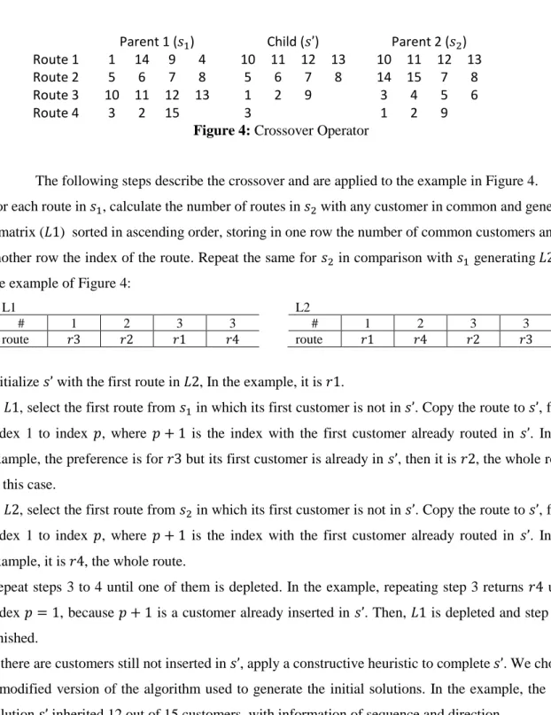
crossover operators that copy routes from both parents, but our operator has a step to reduce the number of conflicts (common customers) while selecting the routes from both parents.

Parent 1 (𝑠1) Child (𝑠’) Parent 2 (𝑠2)

Route 1 1 14 9 4 10 11 12 13 10 11 12 13

Route 2 5 6 7 8 5 6 7 8 14 15 7 8

Route 3 10 11 12 13 1 2 9 3 4 5 6

Route 4 3 2 15 3 1 2 9

Figure 4: Crossover Operator

The following steps describe the crossover and are applied to the example in Figure 4. 1) For each route in 𝑠1, calculate the number of routes in 𝑠2 with any customer in common and generate

a matrix (𝐿1) sorted in ascending order, storing in one row the number of common customers and in another row the index of the route. Repeat the same for 𝑠2 in comparison with 𝑠1 generating 𝐿2. In

the example of Figure 4:

L1 # 1 2 3 3 route 𝑟3 𝑟2 𝑟1 𝑟4 L2 # 1 2 3 3 route 𝑟1 𝑟4 𝑟2 𝑟3

2) Initialize 𝑠’ with the first route in 𝐿2, In the example, it is 𝑟1.

3) In 𝐿1, select the first route from 𝑠1 in which its first customer is not in 𝑠’. Copy the route to 𝑠’, from

index 1 to index 𝑝, where 𝑝 + 1 is the index with the first customer already routed in 𝑠’. In the example, the preference is for 𝑟3 but its first customer is already in 𝑠’, then it is 𝑟2, the whole route in this case.

4) In 𝐿2, select the first route from 𝑠2 in which its first customer is not in 𝑠’. Copy the route to 𝑠’, from

index 1 to index 𝑝, where 𝑝 + 1 is the index with the first customer already routed in 𝑠’. In the example, it is 𝑟4, the whole route.

5) Repeat steps 3 to 4 until one of them is depleted. In the example, repeating step 3 returns 𝑟4 until index 𝑝 = 1, because 𝑝 + 1 is a customer already inserted in 𝑠’. Then, 𝐿1 is depleted and step 5 is finished.

6) If there are customers still not inserted in 𝑠’, apply a constructive heuristic to complete 𝑠’. We choose a modified version of the algorithm used to generate the initial solutions. In the example, the new solution 𝑠’ inherited 12 out of 15 customers, with information of sequence and direction.

5.4– Notes on the features of the local search schemes

In this section, we emphasize the main features that make the proposed algorithms unique when compared with others from the literature. One point is related to the way the local searches are guided. Evolutionary algorithms such as Castro et al. (2011) and Chiang and Hsu (2014) have neighborhood structures that are used as mutation operators not considering the objective function, usually moving to the first feasible solution found, receiving one solution and returning one modified solution. Assis et al. (2013) suggest the adoption of many distinct specialized neighborhoods for each addressed single objective, and the local searches accept the first solution that improves the single objective of the respective local search. In Baños et al. (2013), if the new solution is not dominated by the parents, it is accepted, otherwise the solution is accepted or not according to the criterion of Metropolis in a simulated annealing context.

Qi et al. (2015) force single-objective sub-problems, so the local search is guided as in any typical single-objective approach. Sivaramkumar et al. (2015) normalize the objectives and work with the averages to have single-objective problems, therefore there are no additional challenges while guiding the local search. In Lima et al. (2017), the incumbent frontier set is passed as an input to the local search phase so that the dominance checking can be done along the search inside the neighborhood structure and the local search is performed separately for each objective one at a time.

Differently from those studies, in the current paper, the developed local searches receive one solution and return a local set of non-dominated solutions. In addition to that, the local search accepts the move if the new solution dominates the original solution or if the percentage improvement in one objective is higher than the percentage deterioration in the other objective. Note that this criterion works with the objectives simultaneously, prevents an undesirable zigzag phenomenon and ensures a certain level of quality for the current solution guiding the local search.

Another point is related to the way the local searches are embedded in the framework of the meta-heuristic. Assis et al. (2013) and Lima et al. (2017) count on one VND in their algorithms, but differently, in our proposed MMA we have two sets, working in two phases: pre-intensification and intensification (Algorithm 4). In the first, each solution in ‘Offspring’ is explored by local searches in a way that each solution generates its own local set of non-dominated solutions, that are then merged to form a new ‘Offspring’ comprised of a diverse set of high quality solutions. After that, in preparation for the second VND, these solutions are ranked and the non-dominated solutions form the ‘Offspring rank 1’ that is passed as input for the second VND. Each solution in ‘Offspring rank 1’ is explored by a set of local searches, but differently from the first VND, the local population is initialized with ‘Offspring rank 1’ and it is not reinitialized while interacting over each solution of ‘Offspring rank 1’. This strategy favors diversification in the first VND and intensification in the second VND.

5.5– Multiobjective Evolutionary Algorithm (MOEA)

For comparison purposes, we also implement the Multiobjective Evolutionary Algorithm (MOEA) proposed by Garcia-Najera and Bullinaria (2011) to solve a multi-objective VRPTW. The algorithm comprises a typical evolutionary framework enhanced by a diversification mechanism based on a similarity measure that has outperformed the popular NSGAII. The main loop is presented in Algorithm 6.

Algorithm 6: MOEA

1 Initialize parameters for the VRPTW instance

2 While 𝑔𝑒𝑛 ≤ 𝑛𝑢𝑚𝐺𝑒𝑛

3 if(𝑔𝑒𝑛 = 1) then

4 Generate popSize initial solutions and return Offspring

5 else

6 Apply selection using modified tournament 7 for𝑖 = 1: 𝑛𝐶ℎ𝑖

8 Apply crossover and add child to Offspring

9 end

10 end

11 Offspring'← Mutation(Offspring)

12 _Combine Offspring and Pop

13 _{Cut-off of the population} Pop

14 _{Compute rank and similarity} 15 𝑔𝑒𝑛 ← 𝑔𝑒𝑛 + 1

16 end

In Algorithm 6, line 4, the MOEA starts with a set of popSize solutions, each being a randomly generated feasible route. The parent selection (line 6) consists in a modified 2-tournament method, where the first of two parents is chosen on the basis of rank, and the second on the basis of a similarity measure based on Jaccard’s similarity coefficient, aiming to maintain population diversity. Regarding the crossover operator (line 8), a random number of routes are chosen from the first parent and copied into the offspring, then all those routes from the second parent which are not in conflict with customers already copied from the first, are copied into the offspring. There are three mutation operators: ‘Reallocation’ which takes a number of customers from a given route and allocates them to another, ‘Exchange’ which swaps sequences of customers between two routes, and ‘Reposition’ which selects one customer from a specific route to reinsert it into the same route. In line 12 both populations are combined, and in line 13, when the population size is exceeded in the last selected front, similarity is computed for the solutions in that front, and the least similar are chosen. Finally, line 13 updates the rank and similarity, and line 14 increments the generation counter.

We implement two versions, both using the same operators from Garcia-Najera and Bullinaria (2011) adapted to our problem formulation. The first version (MOEA) works exactly as described in Algorithm 6 (original form), and in the second version (MOEA-VND) we add a VND loop between lines 11 and 12, using the configuration “Pre-Intensification” in Table 1, Section 5.3. The purpose of the second version is to evaluate

whether the inclusion of local searches is able to boost the algorithm’s performance, which we believe is a relevant discussion in terms of algorithm design.

6 – Experiments and Results

This section is divided into four sub-sections with different experiments. Section 6.1 shows the influence of different parameters of the statistical method used to compute the service level. Section 6.2 aims to validate the statistical method by comparing it with a benchmark (method proposed by Zhang et al., 2013). Section 6.3 presents results for some specific features of the optimization algorithms (MMA and MILS), and finally, in section 6.4 we have the application of the algorithms to all Solomon instances.

Regarding the instances for Sections 6.1 and 6.2, all 56 well known Solomon’s benchmark problems with 100 customers were adapted to generate instances with different probabilities of waiting time (from 0 to 100%). Approximately 160 routes were generated for each instance, using the construction heuristic I1 from Solomon (1987), resulting in a database formed by 9037 routes with 3 to 55 customers. For each of the total number of 101701 customers, we calculated 𝑃(𝐴𝑇𝑖≤ 𝑙𝑖) and 𝑃(𝐴𝑇𝑖≤ 𝑒𝑖), i.e., the service level and the

waiting time probability, respectively. We then compute the error of the 203402 calculations as the absolute difference between the computed value and the true value approximated by simulation (Li et al., 2010), using 100000 iterations.

All instances used in the experiments (from Section 6.1 to 6.4) have the same features of the original instances of Solomon, such as vehicle capacity, customer location, time windows and service time. Only a standard deviation for the travel time and service time is added, as explained next.

Let 𝑑𝑖𝑠(𝑖, 𝑗) be the distance between two customers in the original instance, the travel time is a normal distribution left truncated at zero with average 𝐸[𝑇𝑇𝑖,𝑗] = 𝑑𝑖𝑠(𝑖, 𝑗) and standard deviation 𝑑𝑒𝑣[𝑇𝑇𝑖,𝑗]

generated by 𝑈[0.1; 0.6] ∗ 𝑑𝑖𝑠(𝑖, 𝑗) where 𝑈 is a uniform distribution. The service time is also a normal distribution left truncated at zero with average 𝐸[𝑆𝑇𝑖] = 𝑠𝑖 where 𝑠𝑖 is the deterministic service time of the

original instance, and standard deviation 𝑑𝑒𝑣[𝑆𝑇𝑖] = 𝑈[0.1; 0.6] ∗ 𝐸[𝑆𝑇𝑖]. As a reference, the

range 𝑈[0.1; 0.6] is larger than used by Zhang et al. (2013) which was 𝑈[0.2; 0.6]. A second reference is Li

et al. (2010) with a proportion that varies from 0.07 to 0.2 the value of the mean. In Ehmke et al. (2015), the

variation of the travel time is randomly generated uniformly between 0.1 and 0.3. For practical applications, in case service and travel times are Gaussian, we believe it is very unlikely to find a variation outside the range used in this paper.

All algorithms were coded in Matlab R2015a, and tested in a computer dual core Intel i7 2.6 GHz with 16GB RAM, running Windows 10 Pro.

Sections 6.3 and 6.4 report the hypervolume indicator used in Emmerich et al. (2005). Preliminary tests executed Algorithm 1 a number of times in order to have reference points for the max and min values for each objective and for each instance. A normalization is performed on non-dominated solutions for each instance by using 𝑣𝑎𝑙𝑚𝑛𝑒𝑤= (𝑣𝑎𝑙𝑚− 𝑚𝑖𝑛𝑚𝑖 ) ∗ 100 (𝑚𝑎𝑥⁄ 𝑚𝑖 − 𝑚𝑖𝑛𝑚𝑖 ) where 𝑚 is the index for the objective

and 𝑖 is the index for the instance. The reference point is set as (2000, 2000) and the hypervolume is divided by 400 just for better readability.

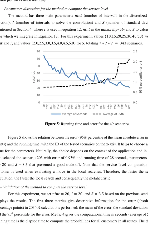
6.1 – Parameters discussion for the method to compute the service level

The method has three main parameters: 𝑛𝑖𝑛𝑡 (number of intervals in the discretized cumulative function), 𝐼 (number of intervals to solve the convolution) and 𝑆 (number of standard deviations), all mentioned in Section 4, where 𝐼 is used in equation 12, 𝑛𝑖𝑛𝑡 in the matrix 𝑚𝑝𝑟𝑜𝑏𝑖 and 𝑆 to calculate bounds

over which we integrate in Equation 12. For this experiment, values (10,15,20,25,30,40,50) were used for

𝑛𝑖𝑛𝑡 and 𝐼, and values (2.0,2.5,3.0,3.5,4.0,4.5,5.0) for 𝑆, totaling 7 ∗ 7 ∗ 7 = 343 scenarios.

Figure 5: Running time and error for the 49 scenarios

Figure 5 shows the relation between the error (95% percentile of the mean absolute error in percentage points) and the running time, with the ID of the tested scenarios on the x-axis. It helps to choose a convenient value for the parameters. Naturally, the choice depends on the context of the application and in this case, it was selected the scenario 203 with error of 0.93% and running time of 28 seconds, parameters 𝑛𝑖𝑛𝑡 = 20,

𝐼 = 20 and 𝑆 = 3.5 that presented a good trade-off. Note that the service level computation in a given customer is used when evaluating a move in the local searches. Therefore, the faster the service level calculation, the faster the local search and consequently the metaheuristic.

6.2– Validation of the method to compute the service level

For this experiment, we set 𝑛𝑖𝑛𝑡 = 20, 𝐼 = 20, and 𝑆 = 3.5 based on the previous section. Table 2 displays the results. The first three metrics give descriptive information for the error (absolute error in percentage points) in 203402 calculations performed: the mean of the error, the standard deviation of the error and the 95th _{percentile for the error. Metric 4 gives the computational time in seconds (average of 5 runs). The} running time is the elapsed time to compute the probabilities for all customers in all routes. The third column

0.0 0.5 1.0 1.5 2.0 2.5 0 10 20 30 40 50 60 70 89 321 108 295 204 49 157 266 152 138 284 162 51 253 203 2 128 128 217 311 224 97 314 46 120 95% p erce n tile (e rro r) se con d s

of the table has the results for the proposed method, the last two columns refer to the benchmark using two configurations for the discrete parameter 𝐿 (the main parameter of the benchmark method).

Table 2: Results for the experiment with benchmark

N Metric Proposed L=10 L=20

1 Mean Error (p.p.) 0.198 0.571 0.245 2 Std. Dev. Error (p.p.) 0.337 0.998 0.427 3 95th Percentile (p.p.) 0.930 2.804 1.168 4 Time (seconds) 27.14 109.43 231.75

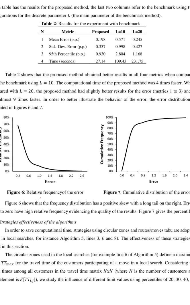
Table 2 shows that the proposed method obtained better results in all four metrics when compared with the benchmark using 𝐿 = 10. The computational time of the proposed method was 4 times faster. When compared with 𝐿 = 20, the proposed method had slightly better results for the error (metrics 1 to 3) and it was almost 9 times faster. In order to better illustrate the behavior of the error, the error distribution is presented in figures 6 and 7.

Figure 6: Relative frequencyof the error :

Figure 7: Cumulative distribution of the error Figure 6 shows that the frequency distribution has a positive skew with a long tail on the right. Errors close to zero have high relative frequency evidencing the quality of the results. Figure 7 gives the percentiles.

6.3 –Strategies effectiveness of the algorithms

In order to save computational time, strategies using circular zones and routes/moves tabu are adopted (used in local searches, for instance Algorithm 5, lines 3, 6 and 8). The effectiveness of these strategies is tested in this section.

The circular zones used in the local searches (for example line 6 of Algorithm 5) define a maximum value 𝑇𝑇𝑚𝑎𝑥 for the travel time of the customers participating of a move in a local search. Considering the

travel times among all customers in the travel time matrix 𝑁𝑥𝑁 (where 𝑁 is the number of customers and each element is 𝐸[𝑇𝑇𝑖,𝑗]), we study the influence of different limit values using percentiles of 20, 30, 40, 50

0% 10% 20% 30% 40% 50% 60% 70% 80% 0.2 0.6 1.0 1.4 1.8 2.2 2.6 Rela tiv e F re qu ency Error 0% 10% 20% 30% 40% 50% 60% 70% 80% 90% 100% 0.0 0.4 0.8 1.2 1.6 2.0 2.4 Cu m u lativ e Fr e q u e n cy Error

and 60%, e.g. 𝑇𝑇𝑚𝑎𝑥 for 60th percentile means 60% of the arcs of the travel time matrix are smaller than 𝑇𝑇𝑚𝑎𝑥.

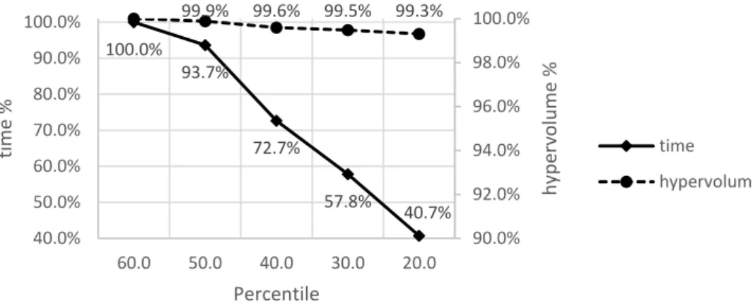
Figure 8 shows the influence of different percentiles used to obtain 𝑇𝑇𝑚𝑎𝑥 in the computational time

and hypervolume of the Pareto front returned by the algorithm. The result from 60th percentile is used as a reference for the other values, dividing the hypervolume obtained with a certain percentile by the hypervolume obtained with 60th _{percentile. Analog for the running time. The results are expressed as the mean of the running} time and hypervolume for five runs of six Solomon instances, the first of each one of the six classes: C101, C201, R101, R201, RC101 and RC201.

Figure 8: Influence of the circular zone

Figure 8 demonstrates that the lower the percentile, the lower the computational time and the lower the hypervolume. For instance, the computational time for the 20th _{percentile is 0.407 times (40.7%) the} running time of 60th _{percentile, while the hypervolume for the 20}th _{percentile is 0.993 (99.3%) the} hypervolume of 60th _{percentile. It is relevant to observe that the reduction of the running time is much bigger} than the reduction of the hypervolume. Therefore, depending on the context of the application, if a small deterioration of the hypervolume is admissible, then it is possible to reduce substantially the computational time with the utilization of the circular zone.

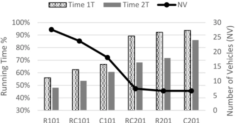
The strategy involving the routes/moves tabu (for example lines 3 and 8 of Algorithm 5) is also tested. Regarding its influence in the hypervolume, hypothesis tests showed no statistical differences for the variance (Levene’s test) and for the mean (ANOVA), with 95% confidence level. Analog tests also showed no statistical difference for the average number of vehicles in the solutions. Figure 9 shows the influence of the routes/moves tabu in the computational time for the same six instances. There are two cases: one using the tabu strategy only for the routes (1𝑇) and another using the strategy for routes and also for moves (2𝑇). The result with no utilization of any tabu strategy is used as reference: 𝑡𝑖𝑚𝑒% = 𝑡𝑖𝑚𝑒(𝑡𝑎𝑏𝑢 𝑐𝑎𝑠𝑒) 𝑡𝑖𝑚𝑒(𝑤𝑖𝑡ℎ𝑜𝑢𝑡 𝑡𝑎𝑏𝑢)⁄ . We also present the average number of vehicles in the solutions.

100.0% 93.7% 72.7% 57.8% _40.7% 99.9% 99.6% 99.5% 99.3% 90.0% 92.0% 94.0% 96.0% 98.0% 100.0% 40.0% 50.0% 60.0% 70.0% 80.0% 90.0% 100.0% 60.0 50.0 40.0 30.0 20.0 h yp erv o lu m e % time % Percentile time hypervolume