WITH ANTILINEAR SYMMETRY
TOM ´AˇS DOHNAL AND PETR SIEGL
Abstract. Many physical systems can be described by nonlinear eigenvalues and bifurcation problems with a linear part that is non-selfadjoint e.g.due to the presence of loss and gain. The balance of these effects is reflected in an antilinear symmetry, like e.g.thePT-symmetry, of the problem. Under this condition we show that the nonlinear eigenvalues bifurcating from real linear eigenvalues remain real and the corresponding nonlinear eigenfunctions remain symmetric. The abstract results are applied in a number of physical models of Bose-Einstein condensation, nonlinear optics and superconductivity, and further numerical analysis is performed.
1. Introduction We consider the nonlinear eigenvalue problem
Aψ−εf(ψ) =µψ, (1)
and analyze the bifurcation inεfrom a simple eigenvalueµ0at ε= 0 in a suitable Hilbert space for a rather general class of densely defined, closed (possibly non-selfadjoint) operators A and locally Lipschitz continuous nonlinearities f, cf. As-sumption (I) below for details. For a homogeneous nonlinearityf, we also consider the additional condition kψk = 1. The main contribution of our paper is to the problem of bifurcation from real eigenvalues under an antilinear symmetry ofAand
f. We show that under this condition the nonlinear eigenvalue remains real and the eigenfunction remains symmetric. This confirms a number of existing numerical computations of specific examples of such a bifurcation problem with an antilinear symmetry, see the references below. Besides presenting the abstract bifurcation results, we explain in detail how these apply to physically relevant examples by checking the assumptions and giving concrete choices of the working space.
The question of real nonlinear eigenvalues in non-selfadjoint problems with sym-metries has gained on physical relevance in the recent years due to the intensive research on nonlinear systems under the parity and time-reversal (PT) symmetry mainly in Bose-Einstein condensates (BECs) [32, 29], nonlinear optics [23], see also [50] for an experimental breakthrough, or superconductivity [48]. In these specific physical problems, the presence of real nonlinear eigenvalues typically means the existence of stationary solutions of the forme−iµtψ(x) withµ∈
Ralso if the system
is subject to balanced gain and loss (modeled by a non-selfadjoint linear part).
Date: April 29, 2015.
2010Mathematics Subject Classification. 47J10, 35P30, 81Q12.
Key words and phrases. bifurcation, nonlinear eigenvalue, non-selfadjoint operator, antilinear symmetry,PT-symmetry.
P.S. thanks G. Wunner and H. Cartarius for drawing his attention to this topic. The research of P.S. is supported by theSwiss National Foundation, SNF Ambizione grant No. PZ00P2 154786. The research of T.D. is partly supported by theGerman Research Foundation, DFG grant No. DO1467/3-1.
1
The interest in antilinear symmetries was initiated by an observation in [4] where Schr¨odinger operators with PT-symmetric complex potentials in the con-text of quantum-mechanics-like linear problems were numerically shown to have real eigenvalues in a certain parameter region.
In the context of BECs, where the (nonlinear) Gross-Pitaevskii equation mod-els the dynamics of the condensate, a complex potential describes the injection and removal of particles and a balance of these two processes is reflected in the
PT-symmetry of the system. Numerical results on the bifurcation of nonlinear eigenvalues in particular in one dimensional models can be founde.g.in [8, 11, 21]. In optics under the paraxial approximation, the system can be modeled by the nonlinear Schr¨odinger equation (NLS) with a potential corresponding to the refrac-tive index, which is complex if the amplification and damping of the light wave are present, a balance is again reflected in the PT-symmetry. Numerical and formal results on the NLS for the bifurcation from linear eigenvalues underPT-symmetry include one dimensional [44, 57, 60] or two dimensional [59].
Superconducting wires driven with electric currents represent another example of a physical application of aPT-symmetric nonlinear eigenvalue problem,cf.[48, 49]. The non-selfadjointness appears due to the dependence of the electric potential on the external current.
As explained in detail in Section 5, our results cover all of the above physical models as they are particular cases of (1) with a linear operator A, a nonlinearity
f and an antilinear symmetryC compliant with the assumptions of our analysis. Our approach to the bifurcation problem (1) is based on the Lyapunov-Schmidt reduction and a fixed point iteration. We decompose the Hilbert space to the one dimensional ker(A−µ0) and its complement using the spectral projection corre-sponding to the eigenvalue µ0and forε >0 we seek solutions (µ, ψ) near (µ0, ψ0), where ψ0 is the eigenfunction of A corresponding to µ0. On the complement of ker(A−µ0) the operatorA−µ0is invertible and a fixed point iteration can be used to obtain a small correction of the eigenfunction for ε small enough. The scalar equation on ker(A−µ0) is solved likewise by a fixed point iteration and it produces a small correction of µ0. In this way we obtain an expansion of µ and ψ up to second order inε.
The problem of bifurcation of nonlinear eigenvalues is of course classical and has been solved,e.g.in [9] for simple eigenvalues in real Banach spaces and in [28] for possibly complex Banach spaces (as relevant in our problem) and for eigenval-ues of odd algebraic multiplicity or for geometrically simple eigenvaleigenval-ues, see [28, Thm.I.3.2]. We choose to prove our results in a Hilbert space and independently of [28] in order to provide an explicit expansion ofµandψand because the Lyapunov-Schmidt reduction and the fixed point equations are used also in the second part on the preservation of the realness of µ under an antilinear symmetry condition. Moreover, we avoid the technical condition kf(ψ)k=O(kψk2) asψ→0 of [28].
For the problem under the assumption of an antilinear symmetryCofAandf, cf.Assumption (II), we check that the fixed point iteration preserves the symmetry of the iterates for ψ and the realness of the iterates forµ. As a result, if µ0 ∈ R
and ifψ0 has the antilinear symmetry, then the nonlinear eigenpair (µ, ψ) satisfies these conditions forεsmall enough too.
To our knowledge the only existing mathematically rigorous papers on similar bifurcation problems under an antilinear symmetry are [31] and [49]. In [31] the concrete example of the discrete NLS with the PT-symmetry is considered. The proof is based on the Lyapunov-Schmidt reduction and the implicit function the-orem. In [49] a one dimensional PT-symmetric nonlinear parabolic problem for
superconducting wires is studied using the center manifold analysis. As a special case, stationary localized solutions are found.
The structure of the paper is as follows. Section 2 presents the assumptions on the operator A and the nonlinearity f in (1) needed for the general bifurcation problem and provides a number of examples ofAandf satisfying these conditions, whereby we concentrate mainly on Schr¨odinger operatorsAbut discuss also a first order Dirac type operator. Section 2 also explains the choice of our function space in which the fixed point iteration is carried out. In Section 3 we prove the bifurcation result and the expansion of the eigenvalue and the eigenfunction. For homogeneous nonlinearities, we rescaleεandψsuch that a solution withkψk= 1 is found. The problem under symmetry assumptions is discussed in Section 4. Both antilinear and linear symmetries are discussed, where the former one is shown to lead to the preservation of the realness of µ. Section 5 explains applications of our results to concrete physical problems from literature. Finally, in Section 6 we present numerical computations of nonlinear eigenvalues of (1) with A = −∆ +V and
f(ψ) =|ψ|2ψinL2(
R2) and withPT-symmetric as well as partiallyPT-symmetric
potentialsV. The effects of a linear symmetry are also observed.
2. Basic assumption and examples of operators and nonlinearities
The following basic assumption comprises a condition on a compatibility of the linear partA with the nonlinearityf and a spectral condition onA.
Assumption (I). LetA be a densely defined, closed operator with a non-empty resolvent set in a Hilbert space (H,h·,·i) with the induced norm k · k, let f be a mapping in H and let (Y,k · kY) be a Banach space. Suppose that the following
conditions are satisfied:
(a) Y is a subspace of H, for some n∈ N is Dom(An) ⊂ Y ⊂ Dom(An−1), and
there arek1, k2>0 such that, for allφ∈Dom(An),
kφkn−1:= n−1 X k=0 kAkφk ≤k 1kφkY ≤k2 n X k=0 kAkφk=:k 2kφkn, (2) (b) µ0 ∈ C is an isolated simple (i.e. with the algebraic multiplicity one)
eigen-value of A. Moreover, suppose that the normalizations of ψ0 ∈ Dom(A),
ψ∗
0∈Dom(A∗),
Aψ0=µ0ψ0, A∗ψ0∗=µ0ψ0∗,
i.e.of the eigenvectors ofA,A∗corresponding toµ0,µ0, respectively, are chosen such that
kψ0k= 1, hψ0, ψ0∗i= 1, (3) (c) the mappingf :Y →Dom(An−1) is Lipschitz in a neighborhood of the eigen-vector ψ0, more precisely: there exist rL > 0 and L > 0 such that, for all
φ, ψ∈ {η∈ Y : kη−ψ0kY < rL},
kf(φ)−f(ψ)kn−1≤k1Lkφ−ψkY. (4)
Remark 2.1 (Remarks on Assumption (I)). The spaceY is our working space in which we perform fixed point iterations. A natural choice for Y is (Dom(A),k · k1), i.e.the domain of A equipped with its graph norm. Nonetheless, it may be convenient to work also with a differentY,e.g.with the form-domain and the norm induced by the quadratic form ofAsince these can be much better accessible than (Dom(A),k · k1) itself, cf. Section 2.1 for examples. Obviously, if the Lipschitz continuity (4) is established with k · kY, it holds also with k · kn. A motivation for consideringn > 1 is given in Examples 2.4 and 2.8, see also Remark 2.9. The
conditionρ(A)6=∅ guarantees that also Dom(An),n >1, is dense in H, therefore alsoY is dense inH.
Recall that ifµ0is a simple isolated eigenvalue ofA, thenµ0is a simple isolated eigenvalue of A∗, cf. [30, Chap.III.6.5-6]; moreover, it can be easily verified that the normalization (3) can be achieved. In detail, hψ0, ψ∗0i= 0 implies that ψ0 ∈ Ker(A−µ0)∩Ran(A−µ0) since Ker(A∗−µ0)⊥= Ran(A−µ0). The eigenvalueµ0 is simple, so Ker(A−µ0)2 = Ker(A−µ0) in particular. From (A−µ0)φ=ψ0 for some φ∈Dom(A) we get (A−µ0)2φ= 0, thusφ=cψ0 and henceψ0= 0, which is a contradiction.
The spectral (Riesz) projectionP0on Ker(A−µ0), defined as a contour integral for sufficiently small δ >0,cf.[30, Chap.III.6], and the complementary projection
Q0:=I−P0can be written, using (3), as
P0:=− 1 2πi Z ∂Bδ(µ0) (A−z)−1dz=h·, ψ0∗iψ0, Q0=I− h·, ψ0∗iψ0. (5) We analyze several groups of operators and nonlinearities below and show that they satisfy Assumption (I). The selection is inspired by various physical models from literature, cf. Section 5, where we apply our results to problems possessing typically additional symmetries, cf.Section 4.
2.1. Schr¨odinger operators and the space Y in Ass. (I).(a). Schr¨odinger operators are naturally associated with the following spaces
(Y,k · kY) = (HsQ(Ω),k · kHs
Q) := ((H
s(Ω)∩Dom(Q)),k · k
Hs+kQ· k), (6)
where Ω is a domain in Rd, s > 0, Q ∈ L2
loc(Ω) and Dom(Q) := {ψ ∈ L 2(Ω) :
Qψ∈L2(Ω)}. It is not difficult to verify that thisY is a Banach space.
Example 2.2 (Schr¨odinger operators with complex potentials, n= 1). Let H=
L2( Rd),V1∈W 1,∞ loc (R d) andV 2∈L2loc(R d). Let V
1andV2 satisfy further (i) ReV1≥0 and|∇V1| ≤C1|V1|+C2 with someC1, C2>0,
(ii) there existα∈[0,1), β≥0 such that, for allψ∈ H2 V1(R
d),
kV2ψk ≤α(k∆ψk+kV1ψk) +βkψk. Then the operator
A:=−∆ +V1+V2, Dom(A) :=H2V1(R d)
and the spaceY =H2 V1(R
d) satisfy Assumption (I).(a) withn= 1. The main step needed to justify (2) is the fact that, for allψ∈Dom(A),
c1kψk2H2 V1 ≤ kAψk2+kψk2≤c 2kψk2H2 V1 ,
where c1,c2>0 are independent ofψ,cf.for instance [6] for details; the standard proof forV1(x) =x2 andd= 1 can be founde.g.in [5, Ex.7.2.4].
Example 2.3 (Schr¨odinger operators with singular potentials,n = 1). LetH =
L2((−r, r)) withr∈(0,+∞],V
1∈L1loc((−r, r)) andv2be a sesquilinear form. Let
V1 andv2 further satisfy
(i) ReV1>0 and|ImV1|<tanθReV1 withθ∈[0, π/2), (ii) H√1
ReV1((−r, r))⊂Dom(v2) and there existα∈ [0,1), β ≥0 such that, for allψ∈ H1√
ReV1((−r, r)),
|v2[ψ]| ≤α(kψ0k2+k
p
Then the m-sectorial operatorAassociated (via the first representation theorem [30, Thm.VI.2.1]) with the closed sectorial form
a[ψ] :=kψ0k2+
Z r
−r
V1(x)|ψ(x)|2dx+v2[ψ], Dom(a) :=H1√ReV1((−r, r)) (8) and the space Y = H1√
ReV1((−r, r)) satisfy Assumption (I).(a) with n = 1. To show (2), recall that, for allψ∈Dom(A)⊂Dom(a),|a[ψ]|=|hAψ, ψi| ≤(kAψk2+
kψk2)/2 and the normsk · k
H1√ ReV1
and p|a[·]|+ck · k2 with a sufficiently large
c≥0 are equivalent,cf.[30, Chap.VI.].
The domain ofaand the spaceY can be selected also, for instance, as
H1√,D ReV1 :=H 1 0((−r, r))∩Dom( p ReV1)
i.e. Dirichlet boundary conditions are imposed at ±r, and the analogues of all claims above remain true.
Example 2.4(Schr¨odinger operators with bounded and regular potentials,n >1).
We present an example of Schr¨odinger operators satisfying Assumption (I).(a) for
n > 1. The motivation for n > 1 comes from the condition s > d/2 for Hs(Rd)
needed for polynomial nonlinearities in Example 2.8 below, guaranteeing that the polynomial nonlinearities satisfy Assumption (I).(c).
Let H = L2(
Rd) and let V ∈ W2(m−1),∞(Rd) for some m ∈ N be a possibly
complex potential. Then the operator
A:=−∆ +V, Dom(A) :=H2(Rd), (9)
and the space and Y =H2n
0 (Rd) =H2n(Rd) satisfy Assumption (I).(a) with any
n≤m. The claim holds since Dom(An) =H2n(
Rd) and, for allψ∈H2n(Rd),
c1kψk2H2n≤ kA n
ψk2+kψk2≤c2kψk2H2n,
where c1, c2 >0. The second inequality above follows from V ∈W2(m−1),∞(Rd)
sinceAnψconsists of terms±∆i1Vj1∆i2Vj2. . .∆inVjnψwithi
k, jk∈ {0,1}for all
k= 1, . . . , nand such that the highest derivative acting onV is of order 2(n−1). Each term can be thus estimated by ckψkH2n. Remaining estimates follow from
the equivalence of norms on H2n(
Rd), seee.g.[12, Lem.3.7.2].
Example 2.5 (Schr¨odinger operators with quasi-periodic boundary conditions).
All examples 2.2, 2.3, and 2.4 can be combined with quasi-periodic boundary condi-tions on a bounded domain Ω⊂Rd. Taking, for simplicity Ω = (−r, r)d, r∈(0,∞),
the quasi-periodicity vectors arek∈(−π, π]d and we can choose
Y=H2V,k 1(Ω) := ψ∈ H2 V1(Ω) :ψ(x+ 2rej) =e ikjψ(x),∇ψ(x+ 2re j) =eikj∇ψ(x) for allj= 1, . . . , dand allx∈∂Ω s.t. x+ 2rej ∈∂Ω}
in Example 2.2, Y=H1√,k ReV1 ((−r, r)) :={ψ∈ H1√ ReV1((−r, r)) :ψ(r) =e ikψ( −r)}
with k∈(−π, π] in Example 2.3 (d= 1), and
Y=H20n,k(Ω) :=
ψ∈H2n(Ω) :Dmψ(x+ 2rej) =eikjDmψ(x) for allj= 1, . . . , d, allm∈Nd s.t. 0≤ |m| ≤2n−1, and for allx∈∂Ω s.t. x+ 2rej ∈∂Ω in Example 2.4. Hereej is thej-th Euclidean vector andDm=∂xm11. . . ∂
md xd .
Example 2.6 (Discrete Schr¨odinger operator). The difference operator on H = Dom(A) =C2N (N ∈ N) defined by (Aψ)n := ψn+1+ψn−1+ iγ(−1)nψn for 2≤n≤2N−1, ψn+1−iγψn forn= 1, −ψn−1+ iγψn forn= 2N, (10)
appears in the modeling of one dimensional optical lattices [31]. ChoosingY =H, assumption (I).(a) is obviously satisfied in this finite dimensional case (e.g. with the Euclidean norm).
Example 2.7 (First order Dirac type operator). An example of a physically inter-esting operator other than a Schr¨odinger one is
A:= −i∂x−V(x) −κ(x) −κ(x) i∂x−V(x) (11) withV, κ∈L∞(R). This operator occurs in a model for optical waves in fibers with
a Bragg grating and a localized defect [22]. Assumption (I).(a) is satisfied under the natural choice H = L2(R)×L2(R),Y = Dom(A) = H1(R)×H1(R), where
kψkY:=kψ1kH1+kψ2kH1.
2.2. The spectral condition (Ass. (I).(b)). To satisfy Assumption (I).(b), a detailed spectral analysis of a given linear operator A must be performed. Here we recall some perturbation results on isolated eigenvalues that can be often used to justify the presence of simple isolated eigenvalues for more complicated, typi-cally non-self-adjoint, differential operators with complex coefficients. In Section 4, Remark 4.3, we further explain the stability of realness of simple eigenvalues if
Apossesses a certain symmetry. Finally, we recall here basic spectral properties of Schr¨odinger operators, particularly the results on the essential spectrum and the simplicity of the ground state.
2.2.1. Holomorphic families of operators. Standard results on the spectrum of a holomorphic family of operators A(γ),γ ∈C, cf.[30, Chap.VII], yield that if the
spectrum of A(0) is separated into two parts, then this remains true also forA(γ) with|γ|sufficiently small,cf.[30, Thm.VII.1.7]. Moreover, isolated eigenvalues de-pend analytically onγand their multiplicities are preserved,cf.[30, Thm.VII.1.8]. Criteria for the holomorphicity of an operator family can be found in [30, Chap.VII]. A sufficient condition for the operators or quadratic forms (and hence for the op-erators associated witha(γ) by the first representation theorem [30, Thm.VI.2.1]) of the type
A(γ) =A0+γB, a(γ) =a0+γb, γ∈C,
where A0 is a densely defined closable operator and a0 is a densely defined clos-able sectorial form, is the relative boundedness of B, b with respect to A0, Rea0, respectively, i.e.
A(γ) : Dom(A0)⊂Dom(B), kBψk ≤αkA0ψk+βkψk, ψ∈Dom(A0),
a(γ) : Dom(a0)⊂Dom(b), |b[ψ]|2≤αRea0[ψ] +βkψk2, ψ∈Dom(a0), with some α, β≥0,cf.[30, Thm.VII.2.6, Thm.VII.4.8].
2.2.2. Spectra of Schr¨odinger operators. We consider Schr¨odinger operators in the setting of Examples 2.2–2.4; many of the following spectral properties are valid in a much greater generality,cf.[20] for instance.
Let A be the operator from Example 2.2 and let lim|x|→∞|V1(x)| =∞. Then the resolvent of A is compact, hence σ(A) = σdisc(A). Moreover, the selfadjoint operator A0 := −∆ +Q, with Q ∈ L2loc(R
d), Q ≥ 0 and lim
has the simple ground state, i.e.the lowest eigenvalue, cf.[47, Thm.XIII.47]. For
d= 1, a Wronskian argument can be used to conclude the simplicity of all eigen-values for single-well potentials like A0 = −∂x2+|x|β, β > 0. For the singular Schr¨odinger operators from Example 2.3, the resolvent is compact if r <∞ (also if Dirichlet or quasi-periodic boundary conditions are considered) or if r=∞and lim|x|→∞|V1(x)| =∞. The simplicity of the ground state in the selfadjoint case can be in some situations concluded from [47, Thm.XIII.48].
LetAbe the Schr¨odinger operator from Example 2.2 withV =V1+V2∈L∞(Rd)
and lim|x|→∞(V1+V2)(x) = 0, thenσess(A) = [0,+∞),cf.[20, Cor.X.4.2, Ex.X.4.3] and e.g. [47, Ex.XIII.4.6]. (Note that there are several different definitions of es-sential spectrum for non-selfadjoint operators, cf. [20, Chap.IX], nevertheless, all coincide for this special situation.) Discrete eigenvalues may appear outside essen-tial spectrum. Particularly ind= 1,2, the selfadjoint operatorA0:=−∆+ε Qwith
R
Qdx <0 andQdecaying sufficiently fast,cf.[53, 33] for precise assumptions onQ, possesses a unique negative simple eigenvalue for all sufficiently small ε >0; some non-self-adjoint extensions can be found in [45, 46]. For the singular Schr¨odinger operators from Example 2.3 withr=∞, σess(A) = [0,+∞) if lim|x|→∞V1(x) = 0 and v2= 0 orv2 are forms corresponding toδpotentials discussed in Section 5.2.
Let A be the Schr¨odinger operator from Example 2.2 with V = V1 +V2 ∈
L∞((−r, r)d) and the k-quasi-periodic boundary conditions, k ∈ (−π, π]d, so, as in Example 2.5, Dom(A) = H20,k((−r, r)d). These operators arise naturally from a periodic problem in L2(
Rd), where V is extended periodically onto Rd cf. [47,
Chap.XIII.16] and the concepts of the “band structure” and of the Bloch eigenvalue problem. As mentioned above, the resolvent of Ais compact. Moreover, if d= 1 and V is real, all eigenvalues ofAare simple ifk /∈ {0, π},cf.[47, Thm.XIII.89]. 2.2.3. Spectrum of the discrete Schr¨odinger operator (10). It is a straightforward calculation, see [31], to show thatA in (10) has the 2N eigenvalues
±4 cos21+2πjN−γ2
1/2
, 1≤j≤N,
which are simple and real for γ∈−2 cos1+2πNN,2 cos1+2πNN.
2.2.4. Spectrum of the Dirac type operator(11). If κ(x)→κ∞>0 andV(x)→0 as |x| → ∞, then the essential spectrum ofAin (11) is (−∞,−κ∞]∪[κ∞,∞). To see this, notice the perturbation result [10, Prop.6.6] and the unitary equivalence of
A in (11) andH in [10] for|x| → ∞. For realκandV the operator is self-adjoint. Bounds on eigenvalues of non-self-adjoint perturbations outside of the essential spectrum are proved in [10]. Special choices of realκandV with simple eigenvalues in (−κ∞, κ∞) have been found in [22, Sec.4.B.] using a connection to the spectral
problem of the inverse scattering theory for the nonlinear Schr¨odinger equation. For example, for κ(x) = (µ20+k2tanh
2
(kx))1/2 andV(x) = k2µ0 2 κ
−2(x)sech2 (kx) with µ0∈(−κ∞, κ∞) and k∈R\ {0}, the operator Ahas a simple eigenvalue at
µ0.
2.3. Nonlinearities (Ass. (I).(c)). We present several nonlinearitiesf satisfying Assumption (I).(c). The considered spaces Y are those arising for Schr¨odinger operators in Section 2.1. In fact, we show that the Lipschitz continuity (4) holds locally for allη0∈ Y, thus also for the eigenvectorψ0.
Example 2.8 (Polynomial nonlinearity). LetH=L2(Ω) andY be as in (6) with s > d/2, s∈N, and Ω =Rd. LetN ∈ Nand fpol(ψ) := N X p,q=0 apqψpψq withapq∈Cbs(R d, C) for all p, q, (12) where Cs
b is the space of functions with continuous and bounded derivatives up to order s. Without any loss of generality, we set a00 = a01 = a10 = 0. A classical example is the cubic nonlinearity fc(ψ) := |ψ|2ψ, i.e. a21 = 1, apq = 0 otherwise. We show below that fpol in (12) satisfies Assumption (I).(c) with any
η0∈ Y=HsQ(R
d) andr L>0.
First note that, for s > d/2, the norm k · kHs satisfies the so-called algebra
property: there exists Ca>0 such that, for all φ, ψ∈Hs(Rd),
kφψkHs ≤CakφkHskψkHs, (13)
cf. [1, Thm.4.39] or [17, Lem.4.2]. Moreover, the Sobolev embedding of Hs(Ω) in L∞(Ω) holds,cf. [1, Thm.4.12], i.e. there exists Ce > 0 such that, for all φ∈
Hs( Rd),
kφkL∞ ≤CekφkHs. (14)
Thus, for allφ, ψ∈ Hs Q(R d), kφψkHs Q =kφψkHs+kQφψk ≤CakφkHskψkHs+ p kφkL∞kψkL∞kQφk kQψk ≤max Ca, Ce √ 2 kφkHs QkψkHsQ, (15)
hence the norm k · kHs
Q satisfies the algebra property as well.
Clearly, it suffices to check (4) for a single termψpψq. From
φpφq−ψpψq= 1 2(φ p −ψp)(φq+ψq) +1 2(φ p+ψp)(φq −ψq), φm−ψm= (φ−ψ) m−1 X k=0 φkψm−1−k (16)
and using (15), we obtain
kφpφq−ψpψqk Hs Q≤C1 kφp−ψpk Hs Qkφ q+ψqk Hs Q+kφ p+ψpk Hs Qkφ q−ψqk Hs Q ≤C2 (kφk q Hs Q+kψk q Hs Q) p−1 X k=0 kφkkHs Qkψk p−1−k Hs Q + (kφkpHs Q +kψkpHs Q ) q−1 X k=0 kφkkHs Qkψk q−1−k Hs Q ! kφ−ψkHs Q,
where C1, C2>0 are independent of φand ψ. Finally, for all ξ∈ {η ∈ HQs(R d) : kη−η0kHs Q < rL}with anyη0∈ H s Q(R d) andr L>0, we havekξkHs Q ≤ kη0kH s Q+rL, thus kφpφq−ψpψqk Hs Q ≤Cη0,rL,p,qkφ−ψkHsQ if φ, ψ ∈ {η ∈ Hs Q(R d) : kη−η 0kHs
Q < rL}. Also note that for a∈ C s b(R d) and ψ∈ Hs Q(Rd) kaψkHs
As a result kfpol(φ)−fpol(ψ)kHs Q ≤ N X p,q=0 kapqkCs(Rd)Cη0,rL,p,q ! kφ−ψkHs Q, (17)
which implies validity of (4) in Assumption (I).(c).
Note that this Lipschitz continuity can be directly extended to vector valued polynomial nonlinearitiesf(ψ) = (f1(ψ), . . . , fm(ψ))T withm∈N,ψ∈(HsQ(R
d))m and withfj(ψ) =PNp1,q1,...,pm,qm=0a (j) p1q1...pmqmψ p1 1 ψ1 q1 . . . ψpm m ψm qm . In the vector case the Hs
Q-norm in (17) must be replaced, e.g., bykψk(Hs Q)m :=
Pm
j=1kψjkHsQ.
Remark 2.9(Motivation forn >1 in Ass. (I).(a)). Examples 2.4 and 2.8 constitute the primary motivation forn >1 in the choice of a spaceY with Dom(An)⊂ Y ⊂ Dom(An−1). The condition
N 3 s > d/2 in Example 2.8 implies that for d≥ 4
we need s ≥ 3. The natural H2-space of Example 2.2 is, therefore, not suitable as our working space. On the other hand, the space H2n of Example 2.4 with
n > d/4 is sufficiently small. The reason for choosing Dom(An)⊂ Y ⊂Dom(An−1) is the use of a fixed point argument in Theorem 3.1, in particular to guarantee
G(Br2ε2)⊂Q0Y, cf.the reasoning between (26) and (27). In summary, if we choose
d
4 <
s
2 ≤n≤mwiths, n, m∈N, (18) then A in (9) with V ∈ W2(m−1),∞(Rd), f = fpol, and Y = H2n(Rd) satisfy
Assumption (I).(a) and (c). Of course, alsoY=H2n,k(Ω) of Example 2.5 with the sameAandfis admissible. Ford= 1,2 inequality (18) holds also withs= 2, n= 1, such thatY=H2
V1(R
d) of Example 2.2 or the spaceH2,k
V1(Ω) of Example 2.5 can be used with f =fpol. Ford= 1 we can use evens= 1, n= 1 and, hence, the spaces
H1√ ReV1((−r, r)),H 1,D √ ReV1((−r, r)) of Example 2.3 andH 1,k √ ReV1((−r, r)) of Example 2.5 are admissible.
Example 2.10 (The monopolar and dipolar interaction from [38, 11]). Let H=
L2(Ω) and Y be as in (6) withs = 2 and Ω =
R3. We investigate nonlinearities
having formally the form (fι(ψ))(x) :=ψ(x)
Z
R3
Kι(y)|ψ(x−y)|2dy, ι∈ {m,d}, with kernels Km(x) = |1x| and Kd(x) = |x1|3
1−3(x.α|x|2)2
with fixed α ∈ R3,
kαkR3 = 1. Notice that choosing K(x) =δ3(x), we can recover also the so called contact interaction, which, however, coincides with the cubic nonlinearity from Example 2.8. Here we focus on the nonlinearitiesfmandfd, the so-called monopolar and dipolar interaction, respectively, see Section 5.2 for more details.
First we show that, for any η∈H2(R3)∩L1(R3),
Z R3 η(x−y) dy |y| L∞ ≤CkηkH2+kηkL1
with C independent ofη. Indeed, the Sobolev embedding (14), applied in the last step, yields Z R3 |η(x−y)|dy |y| = Z B1(0) |η(x−y)|dy |y| + Z R3\B1(0) |η(x−y)|dy |y| ≤ kηkL∞ Z B1(0) dy |y|+kηkL1 ≤CkηkH2+kηkL1.
Using this, the algebra property of k · kH2, cf. (13), the special case of the first formula in (16) and Cauchy-Schwartz inequality, we obtain
kfm(φ)−fm(ψ)k ≤ kφ−ψk Z R3 |φ(x−y)|2dy |y| L∞ +kψk Z R3 |φ(x−y)|2− |ψ(x−y)|2 dy |y| L∞ ≤C1kφk2H2kφ−ψkH2 Q+C2kψkkφ−ψkH2kφ+ψkH2 ≤C3(kφk2H2+kψk 2 H2)kφ−ψkH2 Q,
thus (4) is satisfied with n= 1 for any η0 ∈ HQ2(R3) and rL > 0. In particular, Assumption (I).(c) holds.
The nonlinearity fd is more complicated and it is even not immediately clear why it is well-defined. Nonetheless, the appropriate framework of singular integrals, particularly [54, Thm.II.3], yields that, for anyη∈L2(R3),
Z R3 Kd(y)η(x−y) dy ≤Cdkηk,
withCdindependent ofη. Using the Sobolev embedding (14), the algebra property (13) ofH2-norm and the special case of the first formula in (16), we obtain
kfd(φ)−fd(ψ)k ≤C4(kφk2H2+kψk 2
H2)kφ−ψkH2
Q,
thus (4) is satisfied with n = 1 for any η0 ∈ H2Q(R 3), r
L > 0, and Assumption (I).(c) holds in particular.
Example 2.11 (Nonlocal nonlinearity from [49]). Let H=L2((−1,1)) andY =
H10,D((−1,1)) =H1
0((−1,1)). We analyze the non-local nonlinearity (fN(ψ))(x) :=ψ
Z x
0
Im ψ(s)ψx(s)
ds.
The validity of (4) is easily checked sincefNsatisfies
kfN(φ)−fN(ψ)k = 1 2 (φ−ψ) Z x 0 Im φφx+ψψx ds+ (φ+ψ) Z x 0 Im φφx−ψψx ds ≤ 1 2 kφ−ψkL∞ Z x 0 Im φφx+ψψx ds +kφ+ψkL∞ Z x 0 Im φφx−ψψx ds .
For anyη0∈H01((−1,1)),rL>0 andφ, ψ∈ {η∈H01((−1,1)) : kη−η0kH1< rL}, we have Z x 0 Im φφx+ψψx ds ≤ kkφkkφxk+kψkkψxkk ≤ 1 √ 2 kφk 2 H1+kψk 2 H1 ≤√2(rL+kη0kH1)2 and Z x 0 Im φφx−ψψx ds ≤1 2kkφ−ψkkφx+ψxk+kφ+ψkkφx−ψxkk ≤√2kφ+ψkH1kφ−ψkH1 ≤2√2(rL+kη0kH1)kφ−ψkH1.
Thus, by the embedding of H1 in L∞((−1,1)) as in Example 2.8, we obtain (4).
In summary, Assumption (I).(c) holds with n= 1.
3. Nonlinear eigenvalue problem
First, we prove the local existence and uniqueness of the solutions of the nonlinear eigenvalue problem (1) under Assumption (I). Next, we focus on homogeneous nonlinearities, for which (1) together with conditionkψk= 1 can be solved. Finally, the influence of possible non-selfadjointness (more precisely non-normality) ofAon constants appearing in our estimates is discussed.
3.1. Local existence and uniqueness.
Theorem 3.1. Let A and f satisfy Assumption (I). Then every solution of the nonlinear eigenvalue problem
(A−µ)ψ−εf(ψ) = 0, hψ, ψ∗
0i= 1 (19)
can be written as
µ=µ0+εν+ε2σ, ψ=ψ0+εφ+χ, (20) with ν, σ∈C andφ, χ∈Q0Dom(A) and where
ν =−hf(ψ0), ψ0∗i, (21)
φ is the unique (inQ0Dom(A)) solution of
(A−µ0)φ=νψ0+f(ψ0), (22) and(σ, χ)solves the nonlinear system
0 =εσ+hf(ψ)−f(ψ0), ψ0∗i, (23)
Q0(A−µ0)Q0χ=ε[(ν+εσ)(χ+εφ) +Q0(f(ψ)−f(ψ0))] =:R(χ). (24) Moreover, there exists ε0 > 0 such that, for all ε ∈ (−ε0, ε0), the nonlinear eigenvalue problem (23)–(24)has a unique small solution, namely with
|σ| ≤r1, kχkY ≤r2ε2, where r1, r2=O(1)(ε→0) satisfy(28),(32)respectively.
Proof. Without any loss of generality, for a given (µ0, ψ0) we can write the solution (µ, ψ) as in (20). Although at this point the representation is not unique, we already know that εφ+χ=Q0(εφ+χ) due to the constrainthψ, ψ∗0i= 1 and the normalizationhψ0, ψ∗0i= 1.
First, we apply the projection P0 to (19) and obtain
ν+εσ=−hf(ψ), ψ∗0i=−hf(ψ0), ψ0∗i − hf(ψ)−f(ψ0), ψ0∗i. Definingν :=−hf(ψ0), ψ0∗i, we get equation (23).
Second, we applyQ0 to (19), resulting in
Q0(A−µ0)Q0(εφ+χ) =(εν+ε2σ)(εφ+χ) +εQ0f(ψ)
=ε[(ν+εσ)(εφ+χ) +Q0(f(ψ)−f(ψ0)) +νψ0+f(ψ0)]. Next, we define φto be the unique solution φ∈Q0Dom(A) of (22). This solution exists because νψ0+f(ψ0)∈Ker(A∗−µ0)⊥ = span{ψ∗0}⊥ and becauseµ0 is not in the essential spectrum σe5(A), it is not inσe3(A) either,cf.[20, Chap.IX], and henceA−µ0 is Fredholm. The equation above thus becomes problem (24).
The rest of the proof deals with the existence of a unique solution (σ, χ), withχ
small andσbounded, of (23)–(24). Note thatQ0(A−µ0)Q0is boundedly invertible in Q0H, hence equation (24) can be rewritten as
In the first step, for ε in a small neighborhood of 0, we use the fixed point argument to conclude the existence of a solutionχof (25) withkχkY =O(ε2). We
search for a fixed point
χ∈Br2ε2 :={η∈Q0Y : kηkY≤r2ε
2} (26)
with some r2>0 independent ofε. Its existence is guaranteed if we can show (i) χ∈Br2ε2 ⇒ G(χ)∈Br2ε2,
(ii) there exists ρ ∈ (0,1) such that kG(χ1)−G(χ2)kY ≤ ρkχ1−χ2kY for all χ1, χ2∈Br2ε2.
Note that ψ0, being an eigenfunction, satisfiesψ0 ∈Dom(Am) for any m∈ N.
Thus the right hand side of (22) lies in Dom(An−1), henceφ∈Q
0Dom(An)⊂Q0Y. Therefore if χ∈Q0Y, thenQ0f(ψ)∈Q0Dom(An−1) and R(χ)∈Q0Dom(An−1). It is straightforward to check that thenG(χ)∈Q0Dom(An). The properties of the norm k · kY,cf.Assumption (I).(a), yield
kG(χ)kY≤ k2 k1 kG(χ)kn≤ k2 k1 Cµ0kR(χ)kn−1. (27) To show the second inequality in (27), note that because G(χ)∈Q0Dom(An),
AG(χ) = (A−µ0)Q0G(χ) +µ0G(χ)
=Q0(A−µ0)Q0G(χ) +µ0G(χ) =R(χ) +µ0G(χ). We thus have, for k≥1,
AkG(χ) =Ak−1(R(χ) +µ0G(χ)) =· · ·= k−1 X j=0 µk0−1−jAjR(χ) +µk0G(χ). As a result,kAkG(χ)k ≤Pk−1 j=0|µ0|k−1−jkAjR(χ)k+|µ0|kk(Q0(A−µ0)Q0)−1kkR(χ)k and the second inequality in (27) follows, where Cµ0 >0 is a constant depending on|µ0|, nandk(Q0(A−µ0)Q0)−1k.
To ensure (i), we take χ ∈ Brε2, estimate kR(χ)kn−1 and select suitable r in the following. First note that P0 and Q0 are bounded on Dom(Am), m ∈ N0, moreover, since AkP0ψ=P0Akψ andAkQ0ψ=Q0Akψfor allψ∈Dom(Am) and
k= 0,1, . . . , m, we have kP0km:= sup 06=ψ∈Dom(Am) kP0ψkm kψkm = sup 06=ψ∈Dom(Am) Pm k=0kP0Akψk Pm k=0kAkψk ≤ kP0k,
and similarly kQ0km≤ kQ0k. Next,
kR(χ)kn−1≤ |ε| |ν+εσ|(kχkn−1+|ε|kφkn−1) +kQ0(f(ψ)−f(ψ0))kn−1 ≤ |ε|k1 |ν+εσ|(r2ε2+|ε|kφkY) +kQ0kLkεφ+χkY ≤ε2k1 |ν+εσ|(r2|ε|+kφkY) +kQ0kL(kφkY+r2|ε|) ,
thus we selectr2 such that
r2> k2Cµ0 |ν|+kQ0kL
kφkY. (28)
For all sufficiently smallε, we satisfy firstlykψ−ψ0kY ≤ |ε|kφkY+r2ε2< rL, hence the Lipschitz property of f, cf.Assumption (I).(c), can be indeed used. Secondly we satisfy condition (i).
It remains to prove (ii). Similarly as above, we obtain (withψ1,2:=ψ0+εφ+χ1,2)
kR(χ1)−R(χ2)kn−1=|ε|k(ν+εσ)(χ1−χ2) +Q0(f(ψ1)−f(ψ2))kn−1
≤ |ε|k1 |ν+εσ|+kQ0kLkχ1−χ2kY.
(29) Hence, for all sufficiently small ε, condition (ii) is also satisfied.
In summary, there exists ˜ε0 > 0, such that, for all ε, |ε| < ε˜0, we have the function χ∈Br2ε2 that solves (25); note that then χ∈Q0Dom(A) as well. Note also that χ and in particular ˜ε0 depend onσ. However, we consider only|σ| ≤r1, wherer1satisfies (32), and an inspection of the estimates above shows that we can find ˜ε0 independent ofσ(dependent only onr1).
In order to solve the first equation in (23), we prove first that the solution χis continuous in σ. More precisely,
kχ(σ1)−χ(σ2)kY ≤ k2 k1 Cµ0kR(χ(σ1))−R(χ(σ2))kn−1 =k2 k1 Cµ0|ε|kν(χ(σ1)−χ(σ2)) +ε(σ1χ(σ1)−σ2χ(σ2)) +ε 2(σ 1−σ2)φ +Q0(f(ψ0+εφ+χ(σ1))−f(ψ0+εφ+χ(σ2)))kn−1 ≤k2Cµ0|ε| |ν|kχ(σ1)−χ(σ2)kY+ε2|σ1−σ2|kφkY +|ε| 2 k(σ1−σ2)(χ(σ1) +χ(σ2)) + (σ1+σ2)(χ(σ1)−χ(σ2))kY +kQ0kLkχ(σ1)−χ(σ2)kY ≤k2Cµ0|ε| |ε| 1 2kχ(σ1) +χ(σ2)kY+|ε|kφkY |σ1−σ2| +|ν|+kQ0kL+ |ε| 2 |σ1+σ2| kχ(σ1)−χ(σ2)kY ! , Hence, for |σ1,2| ≤r1, kχ(σ1)−χ(σ2)kY 1−k2Cµ0|ε| |ν|+|ε|r1+kQ0kL ≤k2Cµ0|ε| 3r 2|ε|+kφkY |σ1−σ2|. (30)
As the final step, we use the fixed point argument on
σ=−1
εhf(ψ)−f(ψ0), ψ ∗
0i=:S(σ), (31)
where we search for a fixed point in {σ∈C : |σ| ≤r1} with a suitabler1 selected below. Since
|S(σ)| ≤k1LkP0k(kφkY+r2|ε|), we choose r1such that
r1> k1LkP0kkφkY, (32)
hence, for sufficiently small |ε|, |σ| ≤r1 implies|S(σ)| ≤r1. Moreover, using the continuity ofχin σ,cf.(30), we obtain |S(σ1)−S(σ2)| ≤ 1 |ε|kf(ψ(σ1))−f(ψ(σ2))k ≤ k1L |ε| kχ(σ1)−χ(σ2)kY≤Cε 2 |σ1−σ2|,
hence, for sufficiently small|ε|, the fixed point argument yields the sought solution
3.2. Homogeneous nonlinearity. In the case of a homogeneous nonlinearity like e.g.f(ψ) =|ψ|q−1ψ, solutions with norm one can be generated from the nonlinear eigenfunctions of Theorem 3.1 by a scaling.
Corollary 3.2 (Nonlinear eigenfunction with norm one). Let Aandf satisfy As-sumption(I)and suppose thatf is a homogeneous nonlinearity, i.e.for alla >0, it satisfies the scaling propertyf(aψ) =aqf(ψ)with someq∈
R. Given the nonlinear eigenpair (µ(ε), ψ(ε))for|ε|< ε0 from Theorem 3.1, the pair
(˜µ(˜ε),ψ˜(˜ε)) = µ(ε),kψ(ε)k−1ψ(ε)
withε˜=εkψ(ε)kq−1
solves(A−µ˜) ˜ψ−εf˜ ( ˜ψ) = 0and satisfieskψ˜(˜ε)k= 1. The mappingε7→εkψ(ε)kq−1 is injective for |ε|< ε1, where ε1≤ε0 is small enough.
Proof. From the scaling property we immediately get
(A−µ(ε))kψ(ε)k−1ψ(ε)−εkψ(ε)kq−1f(kψ(ε)k−1ψ(ε)) = 0.
The injectivity follows from the asymptotic equivalence εkψ(ε)kq−1=εkψ
0+εφ+
χkq−1∼εkψ
0kq−1=εforε→0.
Remark 3.3. Similar results on the bifurcation from simple eigenvalues of Fred-holm operators appear in the literature. As mentioned in the introduction, a clas-sical reference is the paper [28] by Ize, where Thm.I.3.2 applies under our assump-tions and the additional condition kf(ψ)k =O(kψk2) as ψ→ 0. The theorem of Ize treats the bifurcation from the zero solution ψ ≡ 0 in (A−µ)ψ = f(ψ) but for a homogeneous f the problem can be rescaled to (1). Our Theorem 3.1 avoids the technical condition kf(ψ)k =O(kψk2) (ψ → 0) and provides a more explicit expansion of µandψ.
3.3. Constants and non-selfadjointness. Our fixed point argument in Theorem 3.1 works for εsufficiently small and the size of remaindersχandσis determined by constants r2 and r1, respectively, cf. (28), (32). Notice that the size of ε is restricted at least by
ε0k2Cµ0 |ν+ε0σ|+kQ0kL
<1,
arising from the contraction condition ρ <1 together with (27) and (29).
Provided A is normal, i.e. AA∗ = A∗A, the spectral projection P0 and the complementary projectionQ0 are orthogonal, hencekP0k=kQ0k= 1, and, in the casen= 1, the constant Cµ0 is determined by spectral properties ofA since
Cµ0 = 1 + (1 +|µ0|)k(Q0(A−µ0)Q0)
−1
k= 1 + 1 +|µ0| dist(µ0, σ(A)\ {µ0})
,
due to the standard relation k(A−z)−1k= dist(z, σ(A))−1 valid for normal oper-ators.
However, in our applications, we usually encounter non-symmetric perturbations of self-adjoint operators that result both in non-selfadjointness and non-normality of the perturbed operators. Note that we lose both equalities for kQ0k andCµ0 if
Ais not normal, only ≥is left in general. In particular, the spectral projections as well as the complementary projections may behave wildly as the size of the spectral parameter is increased even for simple looking one-dimensional Schr¨odinger opera-tors with a complex potential and compact resolvent. For instance, considering the rotated oscillator −∂2
x+ ix
2,cf. [13, 14], for which all eigenvalues λ
n are explicit,
λn=eiπ/4(2n+ 1),n∈N0, the norms of the corresponding spectral projectionsPn grow exponentially, more precisely,
lim n→∞
logkPnk
similar behavior is exhibited also by other well-studied (often PT-symmetric and with real spectrum) Schr¨odinger operators, cf. for instance [26, 27, 43, 36] and references therein. Notice that the growth of kPnk implies the growth of kQnk sincekQnk ≥ kPnk −1. Concerning the size ofCµ0, the norm of the resolvent of a non-normal operator, i.e.its pseudospectrum, see [55], may be dramatically larger than dist(z, σ(A))−1. While there is a collection of recent pseudospectral results for non-normal differential operators,cf.[13, 25, 55], the estimates on the norm of the resolvent of (A−µ0)Q0Dom(A) acting inQ0Hseem not to be available.
On the other hand, there exists a large collection of perturbation results, partic-ularly for operators with compact resolvent,cf.for instance the classical [30, 19, 40] or more recent [52, 58, 2, 3, 42], guaranteeing that the eigensystem of a perturbed selfadjoint (or normal) operator contains a Riesz basis, hence kPnk, kQnk and
k(Qn(A−µn)Qn)−1kare uniformly bounded (kPnkare uniformly bounded already if there is only a basis). The Riesz basis property is present for example for opera-tors in (41), (42), (43) and (50) from Section 5.
4. The role of symmetries
We show that underantilinear symmetry assumptions onAandf,cf. Assump-tion (II) below, the nonlinear eigenvalueµstarting from a real eigenvalueµ0remains real and a certain symmetry of the solutionψis preserved for allε∈(−ε0, ε0). The symmetry of solutions is preserved also in the case of linear symmetries that are studied next.
4.1. Antilinear symmetries.
Assumption (II) (Antilinear symmetries ofAandf). LetAbe a densely defined and closed operator in a Hilbert space H and let C be an antilinear, isometric and involutive operator, i.e.for all φ, ψ ∈ H andλ∈C, C(λφ+ψ) =λCφ+Cψ,
hCφ,Cψi=hψ, φiandC2=I, such that (a) for all ψ∈Dom(A),
Cψ∈Dom(A) and ACψ=CAψ, (33) (b) for allψ∈ Y, where Y is the space from Assumption (I).(c),
Cf(ψ) =f(Cψ). (34) The operator C is referred to as the antilinear symmetry of A and f. The standard example of C is the PT symmetry that is naturally present in various physical models as we indicate in the following example and in Section 5.
Example 4.1 (PT symmetry). Let H= L2(Ω), where Ω =
Rd or Ω = (−r, r)d
with r∈(0,+∞). Define
(Pψ)(x) :=ψ(−x), Tψ:=ψ.
In quantum mechanics, P corresponds to the space reflection (parity) andT is the time-reversal. The antilinear PT symmetry is the composition, i.e.C :=PT. In more dimensional domains, the so called partial PiT symmetries, where
(Piψ)(x1, . . . , xi, . . . , xd) :=ψ(x1, . . . ,−xi, . . . , xd),
are sometimes considered,cf.[7] or [59]. Obviously, alsoPiT is antilinear.
Schr¨odinger operators −∆ +V with complex potentials V, cf. Examples 2.2 and 2.4, are PT-symmetric if V is PT-symmetric, i.e.[PT, V] = 0, or, in other words, the real and imaginary parts of V satisfy (ReV)(−x) = (ReV)(x) and (ImV)(−x) = −(ImV)(x). The Schr¨odinger operators from Example 2.3 posses
this symmetry if, for every φ, ψ ∈ Dom(a), v2(φ,PTψ) = v2(PTφ, ψ) holds, see Section 5 for examples of suchv2.
The polynomial nonlinearity fpol(ψ) from Example 2.8 satisfies Assumption (II).(b) with C = PT if and only if apq(−x) = apq(x) and the space Y can be selected as in Example 2.2, 2.3, 2.4 or 2.5. For the quasi-periodic case in Example 2.5 note that ψ isk-quasi-periodic with a given vectork ∈(−π, π]d if and only if
ψ(−x) isk-quasi-periodic. The monopolar and dipolar interactionsfmandfdfrom Example 2.10 and the nonlocal nonlinearity in Example 2.11 are alsoPT-symmetric as it can be easily checked.
We recall simple facts about spectral properties ofC-symmetric operators.
Lemma 4.2. LetAsatisfy Assumption(II)and letµ0be an eigenvalue ofA. Then (i) µ0 is an eigenvalue ofA and if there is aC-symmetric eigenvector ψ0
corre-sponding to µ0,i.e.
(A−µ0)ψ0= 0, Cψ0=ψ0, (35)
then µ0 ∈ R. Moreover, if µ0 is real and simple, then the corresponding eigenvector can be chosenC-symmetric.
(ii) ifµ0 is isolated simple and real, then, in addition, the spectral (Riesz) projec-tionP0 of Acorresponding to µ0 commutes withC,i.e.
P0C=CP0. (36)
Proof. (i) Let ψe0 ∈ Dom(A), ψe0 6= 0 satisfy (A−µ0)ψe0 = 0. Clearly, by the
C-symmetry ofA,ACψe0=CAψe0=µ0Cψe0, henceµ0 is an eigenvalue ofA. Next, letψ0be as in (35). Then
µ0ψ0=ACCψ0=CAψ0=Cµ0ψ0=µ0ψ0, thusµ0∈R.
Finally, let againψe0 satisfy (A−µ0)ψe0 = 0 and µ0 be simple. It follows from (33) thatACψe0=µ0Cψe0, hence both ofψe0± Cψe0are eigenvectors ofA. However, one of them must be 0 since µ0 is simple. Note that ψe0+Cψe0 is automaticallyC-symmetric and if it is zero, then we take i(ψe0− Cψe0). (ii) Since Acommutes withC, we haveC(A−z)−1= (A−z)−1C. Hence, for the
spectral projectionP0,cf.(5), we get
CP0=−C 1 2π Z 2π 0 (A−(µ0+δeiϕ))−1δeiϕdϕ =− 1 2π Z 2π 0 (A−(µ0+δe−iϕ))−1δe−iϕdϕC =− 1 2π Z 0 −2π (A−z)−1dzC=P0C.
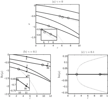
Remark 4.3(Stability of real simple eigenvalues). For aC-symmetric familyA(γ), cf. Section 2.2.1, isolated simple real eigenvalues of A(0) remain isolated simple and real for small |γ| since eigenvalues are analytic inγ and always form complex conjugated pairs,cf.Lemma 4.2.(i).
Notice that many examples in literature as well as in Section 5 can be in fact viewed as a holomorphic family with A(0) =A(0)∗, thus σ(A(0))⊂R. A typical
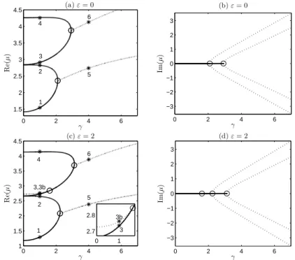
behavior of real eigenvalues as γ is increased, i.e.the non-symmetric part of the operator becomes stronger, is a tendency to merge and create a complex conjugated pair, see e.g.Figure 4 (a), (b).
Finally, we remark that there are alsoC-symmetric (actually withC=PT) oper-ators with real spectrum that are not small perturbations of a selfadjoint operator, e.g.the celebrated imaginary cubic oscillator−∂2
x+ ix3acting inL2(R),cf.[4, 51]. The following theorem shows that real simple eigenvalues µ0 of an operatorA persist to be real nonlinear eigenvalues µ(ε) of A−εf for all ε small enough if
A and f possess anantilinear symmetry. Moreover, starting with a C-symmetric linear eigenfunctionsψ0 ofA(the existence of which is guaranteed by Lemma 4.2), the nonlinear eigenfunctionsψ(ε) are alsoC-symmetric.
Theorem 4.4. Let Aandf satisfy Assumptions (I)and(II). Suppose in addition thatµ0∈Rand choose the corresponding eigenvectorψ0asC-symmetric,i.e.Cψ0=
ψ0. Then, for all ε∈ (−ε0, ε0), the nonlinear eigenpair (µ, ψ) from Theorem 3.1 satisfies µ∈RandCψ=ψ.
Proof. Recall that µ = µ0+εν +ε2σ, ψ = ψ0+εφ+χ and P0 is the spectral projection of Acorresponding to the eigenvalueµ0.
In the first step, we show that ν is real and Cφ =φ. The spectral projection
P0 can be written as P0 = h·, ψ0∗iψ0, where ψ0∗ is as in Theorem 3.1, therefore
−νψ0=P0(f(ψ0)),cf.(21). Using symmetries (34), (35) and (36), we obtain
C(−νψ0) =CP0(f(ψ0)) =P0(f(Cψ0)) =P0(f(ψ0)) =−νψ0, (37) thus −νψ0 =−νψ0, henceν ∈R. ApplyingC to equation (22), using the
symme-tries of A,f andψ0,cf.(33), (34) and (35), we get (A−µ0)Cφ=νψ0+f(ψ0).
Because P0Cφ =CP0φ by (36) and because the solution of (22) withP0φ = 0 is unique, we have Cφ=φ.
Let us now work onσ. Sinceσis the solution of the fixed point problemσ=S(σ) with S(σ) =−1
εhf(ψ(σ))−f(ψ0), ψ
∗
0i, whereψ(σ) =ψ0+εφ+χ(σ) andχ solves the fixed point equation χ = G(χ;σ), it remains to show that the coupled fixed point problem preserves the realness ofσand theC-symmetry ofχ.
Given σ∈R(with|σ| ≤r1), we prove that
Cχ=χ =⇒ CG(χ;σ) =G(χ;σ). (38) As G(χ;σ) = (Q0(A−µ0)Q0)−1R(χ;σ),we first show the analogous property for
R and then the commutation of (Q0(A−µ0)Q0)−1withC. SinceQ0=I−P0, we get from (36) thatQ0C=CQ0 as well. Also note that forCχ=χthe full solution
ψ=ψ0+φ+χisC-symmetric. Hence, forε, σ∈RandCχ=χ,
CR(χ;σ) =ε (ν+εσ)(χ+εφ) +Q0C(f(ψ)−f(ψ0))
=ε (ν+εσ)(χ+εφ) +Q0(f(Cψ)−f(Cψ0))
=R(χ;σ).
To prove (38), it remains to show thatC(Q0(A−µ0)Q0)−1= (Q0(A−µ0)Q0)−1C. To this end, take any ϕ∈Q0H, then
C(Q0(A−µ0)Q0)−1ϕ
= (Q0(A−µ0)Q0)−1(Q0(A−µ0)Q0)C(Q0(A−µ0)Q0)−1ϕ = (Q0(A−µ0)Q0)−1Cϕ.
(39)
Property (38) implies that the fixed point ofχ=G(χ) inBr2ε2,cf.(26), lies in
Br2ε2∩ {η ∈ H:Cη=η}. Finally, we need to show that
Once again, because Cχ=χimpliesCψ=ψ, we get by a straightforward manipu-lation analogous to (37),
C(−εS(σ)ψ0) =CP0(f(ψ)−f(ψ0)) =P0(f(Cψ)−f(Cψ0)) =−εS(σ)ψ0,
henceS(σ)∈Rby the same arguments as below (37).
4.2. Linear symmetries. The operatorAand the nonlinearityf may possess also a linear symmetryS. Then (for simple eigenvalues) symmetry or antisymmetry of the nonlinear eigenfunctions ψ(ε) is preserved as well, however, the preservation of the realness ofµcannot be concluded based solely on a linear symmetry.
Assumption (III) (Linear symmetries of Aand f). Let A be a densely defined and closed operator in a Hilbert space H and let S be a linear, selfadjoint and involutive operator, i.e. for all φ, ψ ∈ H and λ ∈ C, S(λφ+ψ) = λSφ+Sψ,
hSφ, ψi=hφ,SψiandS2=I, such that (a) for all ψ∈Dom(A),
Sψ∈Dom(A) and ASψ=SAψ,
(b) for allψ∈ Y, where Y is the subspace from Assumption (I).(c),
Sf(ψ) =f(Sψ) and f(±ψ) =±f(ψ).
Lemma 4.5. Let A satisfy Assumption (III)and let µ0 be a simple eigenvalue of
A. Then
(i) the eigenvector ψ0, kψ0k = 1, corresponding to the eigenvalue µ0 is either
S-symmetric orS-antisymmetric, i.e.
Sψ0=κψ0, κ= 1or κ=−1.
(ii) the spectral projectionP0 ofA corresponding toµ0 commutes withS,i.e.
P0S =SP0.
Proof. The reasoning is analogous to the one in the proof of Lemma 4.2.
Theorem 4.6. LetAandf satisfy Assumptions(I)and(III). Then the symmetry of the eigenvector ψ0, corresponding to the simple eigenvalue µ0, i.e. Sψ0 =κψ0 withκ= 1orκ=−1, is preserved for the nonlinear eigenfunctionψfrom Theorem 3.1, i.e. Sψ=κψfor allε∈(−ε0, ε0)with the same κ as forψ0.
Proof. Similarly to the proof of Theorem 4.4, we show that Sφ=κφand search for the fixed point in a subsetBr2ε2∩ {η∈ H:Sη =κη}.Note that this is allowed since, similarly as in (38)–(39),
Sχ=κχ =⇒ SG(χ;σ) =κG(χ;σ).
5. Applications
5.1. Toy model. Let H = L2((−r, r)) with r = π/2, γ ∈ C and let Aγ be the m-sectorial operator associated with the form
aγ[ψ] :=kψ0k2+γ |ψ(π/2)|2− |ψ(−π/2)|2
, Dom(aγ) :=H1((−π/2, π/2)). Since V1= 0, we take Y =H10((−π/2, π/2)) =H1((−π/2, π/2)),cf. Example 2.3. Note that the inequality, valid for everyε >0,
kψk2
implies that condition (7) is satisfied. By standard arguments,cf.[30, Ex.VI.2.16],
Aγ=−∂x2,
Dom(Aγ) ={ψ∈H2((−π/2, π/2)) : ψ0(±π/2) +γψ(±π/2) = 0},
(41) and (Aγ)∗ = Aγ, i.e.Aγ is a non-selfadjoint (unless γ ∈ R) perturbation of the
Neumann Laplacian on (−π/2, π/2) in boundary conditions; a collection of spectral results for Aγ can be found e.g. in [35, 37]. The spectrum of Aγ is discrete with explicit eigenvalues:
σ(Aγ) ={−γ2} ∪ {n2}∞n=1.
Forγ= iα, α∈R\Z, the operatorAiα isPT-symmetric,cf.[35] and Example 4.1, and all its eigenvalues are real and simple. Hence the spectral condition in Assumption (I).(b) is satisfied for any µ0 ∈σ(Aiα). The eigenfunctions {ξn}∞n=0,
{ξn∗}∞n=0 ofAiαandA∗iα, respectively, with normalization satisfying (3) read
ξ0(x) = 1 √ πe −iαx, ξn(x) = r 2 π n √ n2+α2 cosnx+π 2 −iα n sin nx+π 2 , n≥1, ξ∗0(x) = απ sin(απ)ξ0(x), ξ ∗ n(x) = n2+α2 n2−α2ξn(x), n≥1.
We consider the cubic nonlinearityfc from Example 2.8 that isPT-symmetric as well, cf. Example 4.1. By Theorems 3.1, 4.4 and Corollary 3.2, we have the nonlinear eigenpair (µ(ε), ψ(ε)) withkψ(ε)k= 1 andµ(ε)∈Rfor anyµ0∈σ(Aiα) and small ε.
Forµ0=n2, n≥1, straightforward calculations lead to
νn=−hξn|ξn|2, ξ∗ni=− 3 2π
and alsoφn can be calculated explicitly by solving (22).
For the special eigenvalueµ0=α2and the corresponding eigenfunctionψ0=ξ0, the normalized nonlinear eigenpair can be found even explicitly, namely
µ(ε) =α2− ε π, ψ(ε) =ψ(0)≡ 1 √ πe −iαx.
Notice the agreement with the expansion of µ and ψ from Theorem 3.1. Indeed, since fc(ψ0) = ψ0/π, identity (21) yields ν0 = −1/π. Equation (22) for φ ∈
Q0Dom(Aiα) then reads
−φ00−α2φ= 0,
henceφ= 0. Moreover,ψ(ε) =ψ(0) implies thatσ= 0 is the fixed point of (31). 5.2. Bose-Einstein condensates with injection and removal of particles. In the physics literature on Bose-Einstein condensates, non-selfadjoint perturbations of harmonic oscillators or Laplacians withδ-interactions are considered; the imaginary part of the linear potential models the injection and removal of particles,cf.[8, 11, 21] for instance.
The nonlinear part of the problem corresponds to the contact (cubic)fc, monopo-lar fm or dipolar fd interaction, cf.Example 2.10; the unit vector αentering the dipolar interaction represents the direction of the polarization, cf.[38, 11]. Spec-tral parameter µ corresponds to the chemical potential, the parameterε controls the strength of the nonlinear interaction and the intensity of particle removal and injection (the non-selfadjoint part of the linear operator) is described by the pa-rameter γ, see (42)–(44). The balance in the removal and injection is reflected in
thePT symmetry of the system (the imaginary part of the potential is odd). One-dimensional examples (obtained by the separation of variables in d= 3 models) of
PT-symmetric linear partsAfrom the literature are the following
−∂x2+x2+v0e−σx 2
+ iγxe−ρx2, γ, v0∈R, ρ≥0, (42)
−∂x2+x2+ iγ(δ(x−τ)−δ(x+τ)), γ∈R, τ >0, (43)
−∂x2−(1−iγ)δ(x−τ)−(1 + iγ)δ(x+τ), γ∈R, τ >0. (44) Notice that all can be viewed as holomorphic operator families A(γ) with A(0) =
A(0)∗,cf.Section 2.2.1.
Model (42) corresponds to an operatorAfrom Example 2.2 withσ(A) =σdisc(A), cf.Section 2.2.2. Forv0and|γ|small, all eigenvalues ofAare simple and real,cf. Re-mark 4.3, moreover, it followse.g.from [42] that the number of non-real eigenvalues is finite for any v0, γ ∈R; a numerical analysis of eigenvalues for (42) can be found
in [11].
Models (43)–(44) correspond to the singular Schr¨odinger operator from Example 2.3. Both can be introduced through the closed sectorial form a, cf. (8), namely
V1(x) =x2, v2[ψ] = iγ(|ψ(τ)|2− |ψ(−τ)|2 for (43) andV1(x) = 0, v2[ψ] = (−1 + iγ)|ψ(τ)|2−(1 + iγ)|ψ(−τ)|2 for (44). Note that condition (7) is satisfied (for any
γ ∈ C) because of (40). For (43), the spectrum is purely discrete and real for
sufficiently small |γ|, cf. Section 2.2.2 and Remark 4.3, the number of non-real eigenvalues is finite for anyγ∈R,cf.[41] for a detailed spectral analysis and [24] for a numerical analysis of eigenvalues. The essential spectrum for (44) is equal to [0,+∞) and discrete eigenvalues outside of [0,+∞) may appear, cf. Section 2.2.2 and Remark 4.3. In more detail, if
(1 +γ2)τ >1 and (1 +γ2)e−2τ> γ2,
then there are two negative eigenvalues that are obtained as solutions µof
e−4τ √ −µ= 4 1 +γ2 −µ−√−µ+γ 2 4 ,
cf.[34, 39]. A numerical analysis of eigenvalues of (44) can be found in [8]. In summary, Theorem 3.1, Corollary 3.2 and Theorem 4.4 prove the effects ob-served in physics literature, i.e.for ε 6= 0, nonlinear eigenvalues are shifted with respect to linear ones and thoseµthat start from real simple linear eigenvaluesµ0 are real and thePT symmetry of the nonlinear solutionψ is preserved. Note that the latter applies for all nonlinear interactionsfpol,fmorfdmentioned above and a collection of Schr¨odinger operators in Examples 2.2 and 2.3.
A numerical analysis of a model with d = 2, which is qualitatively similar to (42), is performed in Example 6.1.
5.3. Spin-orbit-coupled Bose-Einstein condensate. The spin-orbit-coupled Bose-Einstein condensate is described by the spinor φ ∈ H :=L2(R)×L2(R) obeying
the equation i∂tφ=Aφ+εf(φ) with A= −∂2 x+V(x) + iγ ω+ iκ∂x ω+ iκ∂x −∂x2+V(x)−iγ , f(φ) = (|φ1|2+|φ2|2)φ1 (|φ1|2+|φ2|2)φ2 (45) where V is a trap potential satisfying the conditions in Example 2.2, κ∈Ris the
strength of the spin-orbit coupling, ω ∈ R is the strength of the linear Zeeman
decay and the gain of the (pseudo-)spin states up and down, respectively, cf.[29]. The time harmonic ansatz φ(x, t) =e−iµtψ(x) leads to the eigenvalue problem (1). Since the off-diagonal part ofAis relatively bounded with respect to the diagonal part (i.e.two copies of a Schr¨odinger operator from Example 2.2) with the bound 0, the operator A in (45) with Dom(A) = H2
V1(R)× H 2
V1(R) has the graph norm equivalent to kψkY := kψ1kH2
V1
+kψ2kH2
V1
, see Example 2.2. Moreover, A has compact resolvent if |V1(x)| → ∞as|x| → ∞and it is self-adjoint for realV and
γ= 0. Hence, real simple eigenvalues (if any) ofAforγ= 0 stay simple and real for
γsmall,cf.Remark 4.3. For instance, ifV(x) =x2, then, forγ= 0, the eigenvalues of A read 2n+ 1±ω−κ2/4, n∈N0 and are all simple if ω 6= 0, cf. [29]. Notice that the nonlinearity f from (45) satisfies Assumption (I).(c) with Y := Dom(A),
k · kY as above,cf.the remark on the vector case at the end of Sec. 2.8.
IfV isPT-symmetric,i.e.V(x) =V(−x), the operatorAand the nonlinearity
f in (45) possess a natural antilinear symmetry (Cψ)(x) :=σ1ψ(−x), where σ1 is the Pauli matrix, being the composition of the parity, time and charge symmetries, cf. [29]. Hence our results show the existence of the stationary nonlinear modes bifurcating from the linear ones, particularly for the parabolic trap V(x) = x2 investigated in [29].
5.4. Optics: nonlinear Schr¨odinger-type equations. Another set of physical applications of nonlinearPT-symmetric problems is optics,cf.for instance [44, 59], where light propagation is modeled by nonlinear Schr¨odinger-type equations
i∂zu+ ∆u−V(x)u+f(u) = 0, with a gauge invariant f, i.e.f(eiαu) =eiαf(u) for all α∈
R, and typically with
V ∈L∞(Ω). The variablezis the propagation direction of the optical waves. The real part of the optical potential V corresponds to the refractive index and ImV
models the gain and loss of the medium. If the latter is balanced, in the sense that (ImV)(−x) = −(ImV)(x), and if, in addition (ReV)(−x) = (ReV)(x) and
f isPT-symmetric, then the whole system isPT-symmetric. For a heterogeneous material,V can generally be discontinuous and, in that case, the decomposition to
V1 and V2 complying with V1∈Wloc1,∞(R
d) must be selected to fit into the setting of Example 2.2; however notice that any boundedV fits there after settingV2=V. The physically most usual nonlinearity isfc,i.e.the cubic one,cf.Example 2.8.
Examples of smoothV in d= 2 from [59] and ind= 1 from [44] are
V(x1, x2) =−(v0+ iγx1x2)e−x 2 1e−x22, γ, v 0∈R, (46) V(x1, x2) =−3v0 e−(x1−a)2−(x2−a)2+e−(x1+a)2−(x2−a)2 −2v0 e−(x1−a)2−(x2+a)2+e−(x1+a)2−(x2+a)2 −2iγe−(x1−a)2−(x2−a)2−e−(x1+a)2−(x2−a)2 −iγe−(x1−a)2−(x2+a)2−e−(x1+a)2−(x2+a)2, γ, v 0, a∈R, (47) V(x) =−cos2(x)−iγsin(2x), γ∈R. (48)
Once again, like for Bose-Einstein condensates, the parameter γ determines the strength of non-selfadjointness, i.e.the loss and gain here, and all models can be viewed as holomorphic operator familiesA(γ) withA(0) =A(0)∗,cf.Section 2.2.1. The potentialV satisfies|V(x)| →0 as|x| →+∞for both (46) and (47), hence the essential spectrum of corresponding A(γ) is [0,∞), cf. Section 2.2.2. Since
R
eigenvalues ofA(0) =−∆ + ReV, which are simple for sufficiently smallv0,cf. Sec-tion 2.2.2. Neither one of the potentials (46) and (47) is PT-symmetric but both are P1T-symmetric and (46) is also P2T-symmetric, cf. Example 4.1, hence the simple real eigenvalues of A(0) remain simple and real for sufficiently small |γ|, cf.Remark 4.3.
Regarding periodic problems, likee.g.(48), our results are relevant for the Bloch eigenvalue problem. In the case of A = −∂2
x+V(x) with a 2π-periodic V, one considers the family of operatorsA inL2((−π, π)) withk-quasi-periodic boundary condition,i.e.with the domain
Dom(A) ={ψ∈H2((−π, π)) :ψ(π) =eikψ(−π), ψ0(π) =eikψ0(−π)}
and the form domain H10,k((−π, π)), cf. Example 2.5. Since V in (48) is PT -symmetric, eigenvalues ofAfork /∈ {0, π}are simple and real for sufficiently small
|γ|, cf. Section 2.2.2 and Remark 4.3. Numerical analysis from [44] suggests that for (48) this is the case if|γ|<1/2.
In summary, our results in Theorem 3.1, Corollary 3.2 and Theorem 4.4 are applicable and provide for (46) and (47) and any f compatible with Assumptions (I) and (II) real nonlinear eigenvaluesµof−∆ψ+V ψ−εf(ψ) =µψwith nonlinear solutionsψthat satisfy the corresponding partialPT symmetries. For the periodic problem (48), we obtain nonlinear Bloch functions ψ(x) =p(x)eikx, wherepis 2π -periodic. This complements the results of [18] on the bifurcation of nonlinear Bloch waves in the selfadjoint case. In the z-dependent nonlinear Schr¨odinger equation we obtain solutionsu(z, x) =e−iµzψ(x) with a real propagation constantµdespite the fact that the material exhibits loss and gain.
A numerical analysis of the model with the potential in (47) is performed in Example 6.2.
5.5. Optics: discrete nonlinear Schr¨odinger equation. The propagation of light in a finite one dimensional lattice of linearly coupled Kerr-nonlinear fibers is often modeled by the discrete nonlinear Schr¨odinger equation
i∂zun=un+1+un−1+ iγ(−1)nun+|un|2un, 1≤n≤2N, u0=u2N+1= 0, where z is the propagation direction, n ∈N is the lattice site and iγ(−1)n ∈ iR
describes the loss or gain at the site n, see [31]. For time harmonic solutions
un(t) =e−iµtφn and after the rescaling ψn :=ε−1/2φn (withε >0), we get eigen-value problem (1) with A in (10) and the nonlinearity fn(ψ) = |ψn|2ψn. Exam-ple 2.6 and Section 2.2.3 explain that for |γ| small enough Assumption (I) holds with H = Y := C2N. Note that the Lipschitz continuity of f holds, e.g. with
P2N j=1 |ψn|2ψn− |φn|2φn 2 ≤cmaxj=1,...,2N{|ψn|4,|φn|4}P 2N j=1|ψn−φn|2.
Assumption (II) is satisfied with (Cψ)n =ψ−n (i.e.the discretePT-symmetry) due to the choice of the “potential” Vn := iγ(−1)n, such that V−n = Vn. Our results therefore recover Theorem 1 in [31].
5.6. Optics: coupled mode equations. In Kerr-nonlinear optical fibers with a Bragg grating and a localized defect the propagation of asymptotically broad wavepackets can be described by the system of “coupled mode equations”
i(∂tE1+∂xE1) +κ(x)E2+V(x)E2+ (|E1|2+ 2|E2|2)E1= 0 i(∂tE2−∂xE2) +κ(x)E1+V(x)E1+ (|E2|2+ 2|E1|2)E2= 0
withκ(x)→κ∞>0 andV(x)→0 as|x| → ∞, see [22]. The potentialsκ(x)−κ∞
and V(x) describe the defect of the material and are determined by the refractive index. Once again, we consider the time harmonic ansatzE(x, t) =e−iµtφ(x) and
after the rescalingψ:=ε−1/2φ(withε >0), we obtain eigenvalue problem (1) with A in (11) and f(ψ) = (|ψ1|2+ 2|ψ2|2)ψ1 (|ψ2|2+ 2|ψ1|2)ψ2 .
As mentioned in Section 2.2.4, real smooth and bounded potentials κandV exist such thatAhas a simple isolated eigenvalue. Examples 2.7 and 2.8 (see the remark on the vector case at the end of Sec. 2.8), guarantee that Assumption (I) is satisfied with H = L2(R)×L2(R) and Y = H1(R)×H1(R) provided V, κ ∈ L∞ and
κ(x)→κ∞>0 andV(x)→0 as|x| → ∞.
For materials with loss/gain the potentialsV andκbecome complex and choos-ing them PT-symmetric, we satisfy also Assumption (II). The existence of a real simple isolated eigenvalueµ0 ofA is guaranteed at least for small imaginary parts of κandV by the analytic dependence as in Remark 4.3. Hence, (in the language of [22]), our results show that conservative nonlinear defect modes bifurcate from linear ones in thePT-symmetric case.
5.7. Superconductivity. A model of a finite superconducting wire is discussed in [48, 49] and the bifurcation of nonlinear states for a nonlinear parabolic equation (d= 1) on Ω = (−1,1) is studied. In detail, the problem
wt=wxx+ ixIw+ Γw+N[w], x∈(−1,1), w(−1) =w(1) = 0, N[w] =−|w|2w+ iwZ x 0 Im (w(s, t)wx(s, t)) ds, (49)
where I and Γ are real parameters, is considered. In [49, Sec.6] the authors study the bifurcation of nonlinear (generallyt-dependent) solutions from the zero solution at the smallest eigenvalueλ1∈Rof
A:=−∂2
x−ixI, Dom(A) :=H2((−1,1))∩H01((−1,1)). (50) The potential −ixI is PT-symmetric, so the spectrum of A remains real if the parameter I is chosen small enough, cf. Remark 4.3, and the number of non-real eigenvalues remains finite for any I∈R. For the bifurcation problem the authors
set Γ = Reλ1+ε,0< ε1 and use the center manifold reduction, where the center manifold is one dimensional and corresponds to the zero eigenvalue of A−Reλ1. On the manifold they study t-dependent, but also stationary nonlinear solutions. The asymptotics of the latter are given by
w(x)∼ε1/2αu1(x),
where u1 is the linear eigenfunction corresponding to λ1 and α ∈ R is the
pro-jection coefficient on the center subspace and solves an algebraic equation. For
I small enough λ1 ∈ R, such that a real nonlinear eigenvalue Γ bifurcates. The
eigenfunctionwisPT-symmetric due to thePT-invariance of the center manifold. In the formal part of [49] the more detailed expansion
w(x)∼ε1/2αu1(x) +ε3/2w1(x), is given, where the correctionw1 solves
(A−λ1)w1=αu1+N[αu1]. (51)
α∈Rcan then be selected via the solvability condition of the above equation and
agrees to leading order with theαfrom the center manifold approach.
To relate this work to our results, we rescale thet-independent solutionw(x) =
ε1/2ψ(x) and recover from (49) a problem of type (1), namely (A−Γ)ψ−ε fc(ψ) +fN(ψ)
cf. Examples 2.8, 2.11. Equation (51) thus corresponds to our (22). Observe that A fits into the setting of Example 2.3 with V1(x) = ixI, v2 = 0 and Y =
H10,Dir((−1,1)) =H01((−1,1)). The nonlinearities are discussed in Examples 2.8, 2.11 and 4.1 and it shown thatH1is a suitable space for the Lipschitz condition (4). Hence, our results in Theorem 3.1, Corollary 3.2 and Theorem 4.4 are applicable and provide real nonlinear eigenvaluesµwithPT-symmetric nonlinear solutionsψ.
6. Numerical Examples
We analyze numerically two nonlinear problems of type (1), both with the Schr¨odinger operator A = −∆ +V in L2(R2), cf. Example 2.2, and the cubic
nonlinearity fc,cf.Example 2.8,i.e.
(−∆ +V)ψ−ε|ψ|2ψ=µψ, kψk
L2 = 1. (52)
Selected potentials V posses some antilinear or linear symmetries. Clearly, the nonlinearity is highly symmetric and satisfies Assumption (II).(b) with C = PT
as well as C =PjT, j = 1,2, and also Assumption (III).(b) with any coordinate reflection symmetryS.
Our choice of d = 2 rather than the numerically simpler d = 1 allows the investigation of partial PT-symmetries as well as the interplay between antlinear and linear symmetries in a single problem.
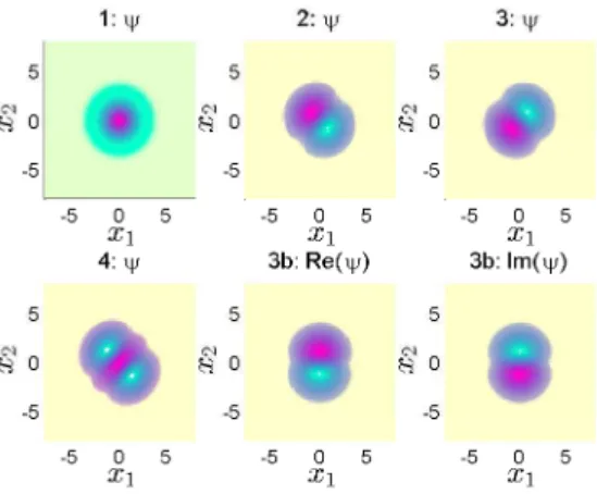
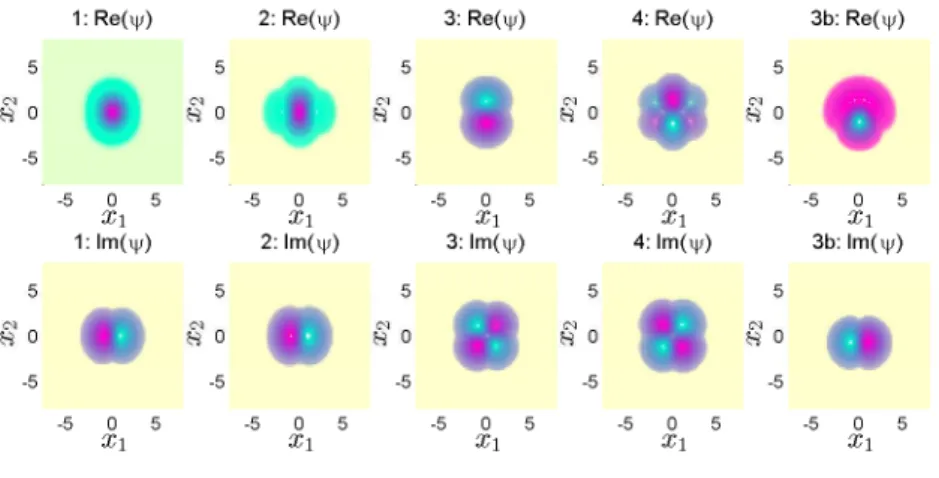
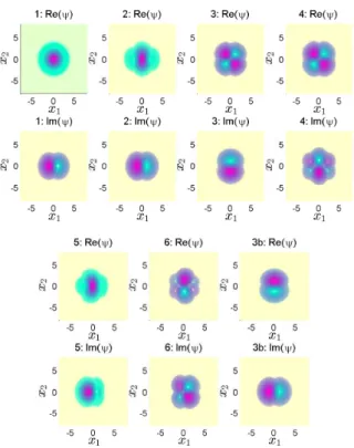
The numerics are performed using the packagepde2path[56, 15, 16] for numeri-cal continuation and bifurcation in nonlinear elliptic systems of PDEs. The package uses linear finite elements for the discretization, Newton’s iteration for the compu-tation of nonlinear solutions and an arclength continuation of solution branches. In all numerical computations, the free complex phase of the solution was fixed by forcing Im(ψ(x0)) = 0 at a selected point x0 within the computational domain. For the plots, we selectx0= (0,0) for thePT-symmetric case in Example 6.1 and
x0 = (0,2) for the P1T-symmetric Example 6.2. In all computations, except for one case mentioned below, the numerical grid is selected symmetric with respect to both coordinate axes as well as with respect to the reflection x→ −x. This is crucial for recovering symmetries of eigenfunctions and realness of eigenvalues.
Example 6.1. We consider first the following imaginary perturbation of the har-monic oscillator that is compatible with Example 2.2 and inspired by the Bose-Einstein condensates models from Section 5.2,
V(x1, x2) = 1 2(x 2 1+x 2 2) + iγx1 2 x2 1+x22+ 2 . (53)
Clearly, V(−x1,−x2) = V(x1, x2) = V(−x1, x2). Hence, the problem has three symmetries: two antilinear symmetries, namely the PT symmetry and the P1T symmetry, and the linear P2 symmetry,cf.Example 4.1.
Forγ= 0, the eigenvalues ofA are known explicitly:
λk =
√
2k, k= 1,2, . . . , where the multiplicity ofλk isk.
Enumerating the eigenvalues including their multiplicity, we obtain our eigenvalues
µn forε=γ= 0.
For the discretization of the PDE, we take 2∗802= 12800 isosceles right triangles of equal size generated by Matlab’s commandpoimeshon the domainx∈[−8,8]2 with homogeneous Dirichlet boundary conditions. The first four eigenfunctions are well localized within the selected domain.
Forγ= 2, the numerically obtained first four eigenvalues (forε= 0) are
µ1≈2.096, µ2≈2.583, µ3≈3.155, µ4≈4.256, and they are all simple.
0 2 4 6 8 10 −1 0 1 2 3 4 ε µ (a)γ= 0 1 2,3 4 3b 0 0.5 2.8 2.85 0 2 4 6 8 10 −1 0 1 2 3 4 ε µ (b)γ= 2 1 2 3 4 3b 4.6 4.8 5