Hamming Distance Kernelisation via Topological
Quantum Computation
Alessandra Di Pierro1, Riccardo Mengoni1, Rajagopal Nagarajan?,2 and David Windridge??,2
1
Dipartimento di Informatica, Università di Verona, Italy 2
Department of Computer Science, Middlesex University, London, UK
Abstract. We present a novel approach to computing Hamming dis-tance and its kernelisation within Topological Quantum Computation. This approach is based on an encoding of two binary strings into a topo-logical Hilbert space, whose inner product yields a natural Hamming distance kernel on the two strings. Kernelisation forges a link with the field of Machine Learning, particularly in relation to binary classifiers such as the Support Vector Machine (SVM). This makes our approach of potential interest to the quantum machine learning community.
Keywords: quantum computing, topology, kernel function
1
Introduction
The Hamming distance of two strings is defined as the number of positions in which the strings are different. It was introduced in the context of error detect-ing and error correctdetect-ing codes [8]. The concept is widely applicable to diverse areas such as information theory, coding theory, cryptography and telecommuni-cation. As well as its use throughout computer science, the Hamming distance is interesting from the perspectives of statistical data analysis and machine learn-ing in that it constitutes a simple (in fact the simplest) instance of a kernel distance. Kernel distances are built from kernel functions via the metric relation
D(x, y) =K(x, x) +K(y, y)−2K(x, y). Critically, from our perspective, kernel functions can be shown to be equivalent to an inner product within a space produced via the kernel function’s implicit feature mapping, thereby enabling e.g. linear learning algorithms to learn highly non-linear decision boundaries. In many applications where data classification is based on dissimilarity mea-sures (e.g. string matching for pattern recognition), kernels provide a method for classification and regression in the absence of obvious features.
In this paper we show that there is a strong relationship between Ham-ming distance and Topology and we use it to define a quantum algorithm that
?
Partially supported by EU ICT COST Action IC1405 “Reversible Computation— Extending Horizons of Computing".
??
Supported by EU Horizon 2020 research project No. 731593 “Dream-like simulation abilities for automated cars (DREAMS4CARS)".
computes a Hamming distance based kernel. Topology is the branch of Math-ematics in which two objects are identified whenever one can continuously be deformed into the other. It has been used in physics to define a very particular class of quantum field theories, namely the Topological Quantum Field Theo-ries (TQFTs), modelling phenomena such as the fractional quantum Hall effect. Quantum computers can benefit from the use of topological properties in as far as they can guarantee a form of robustness [14]. This is possible because in a topological quantum computer information is encoded in the collective states of many quasi-particles, so-called anyons, which are naturally protected from decoherence by their braiding behaviour.
Topological Quantum Computation (TQC) is equivalent in computational power to other standard models of quantum computation such as the quantum circuit model and the quantum Turing machine model. However, certain algo-rithms are more naturally implementable on a topological quantum computer. A well known example of such an algorithm is the one for evaluating a knot invariant called the Jones polynomial [7,2]. The quantum algorithm we present is essentially the application of the Jones polynomial algorithm after an appro-priate problem reduction. This is obtained by an encoding of binary strings as some special braiding in TQC and deriving their Hamming distance as the Jones polynomial of a particular link. We can then exploit the computational features of TQC for comparing two strings and obtain an estimation of the Hamming dis-tance between them. Moreover, the encoding function corresponds to the feature map of a kernel defined as the dot product in the Hilbert space of the topological quantum algorithm (i.e. the feature space). This demonstrates the suitability of TQC for defining kernel methods in a natural way.
2
Preliminaries
In this section we briefly review the main concepts in Topology that are relevant for the work presented in this paper, namely those of knots/links, braiding and related results.
Knot theory [1,12] studies the topological properties of mathematical knots and links. A knot is an embedding of a circle in the 3-dimensional Euclidean spaceR3, up to continuous deformations, and a link is a collection a knots that may be linked or knotted together. A fundamental question in knot theory is whether two knot diagrams, i.e. projections of knots on the plane, represent the same knot or rather they are distinct. The Reidemeister theorem [16] says that two links can be continuously deformed into each other if and only if any diagram of one can be transformed into a diagram of the other by a sequence of moves called Reidemeister moves [17]. If there exists such a transformation the two links are said to be isotopic.
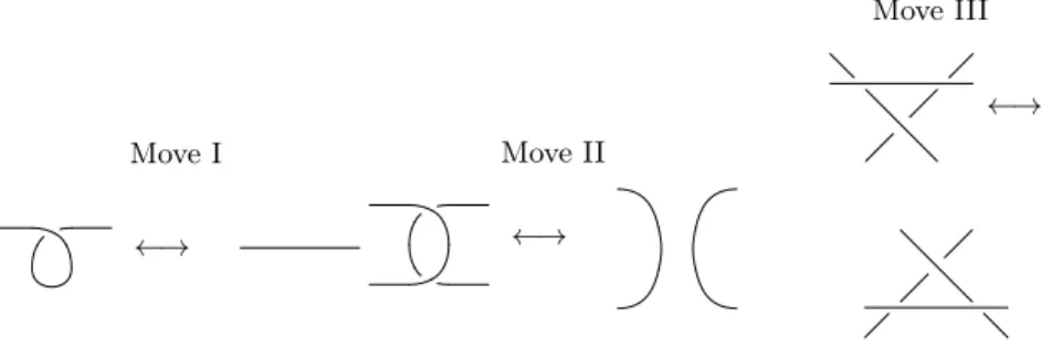
The Reidemeister moves can be of three types, as depicted in Figure 2. Move I undoes a twist of a single strand, move II separates two unbraided strands and finally move III slides a strand under a crossing. A powerful knot invariant is the Jones polynomialVL(A)[9] which is a Laurent polynomial in the variable A
Move I ←→ Move II ←→ Move III ←→
Fig. 1.The Reidemeister moves
with integer coefficients. Given two links L1 and L2 and their respective Jones polynomialsVL1(A)andVL2(A), the following relation holds true:
L1=L2 ⇒ VL1(A) =VL2(A)or, equivalently,VL1(A)6=VL2(A) ⇒ L16=L2. A useful formulation of this polynomial due to Kauffman [10,11] is given in terms of the so-called bracket polynomial or Kauffman bracket, defined in the following section. Crucial for our work is that such a polynomial can be efficiently computed in TQC [2].
2.1 Kauffman Bracket
Definition 1. The Kauffman bracket of any (unoriented) link diagram D, de-notedhLi, is a Laurent polynomial in the variable A, characterized by the three rules:
1.
= 1, where is the standard diagram of the loop 2.
Dt
= (−A2−A−2)hDi=dhDi, where t denotes the distant union3
and(−A2−A−2) =d.
3. D E=AD E+A−1D E
where and represent some regions of link diagrams where they differ as shown.
Rule3 expresses the skein relation: it takes in input a crossingri and dissolves it generating two new links that are equal to the original link except forri, and therefore with a smaller number of crossings. By applying it recursively to a link we obtain at the end a number of links with no crossings but only simple
3 The distant union of two arbitrary links L and M, denoted byLtM is obtained by
first moving L and M so that they are separated by a plane, and then taking the union.
loops, though this number is exponential in the number of crossings. Rule 1 and Rule 2 show how to calculate the polynomial after the decomposition achieved by applying Rule 3.
Note that the Kauffman bracket of a link diagram is invariant under Reide-meister moves II and III but it is not invariant under move I.
Proposition 1. For every two links L and M, the distant unionLtM has the property:
hLtMi= (−A2−A−2)hLi hMi=dhLi hMi
The Kauffman Bracket of the Hopf link We show here the calculation of the Kauffman bracket for the simplest non-trivial link with more than one component, i.e. the Hopf link depicted below [15].
By applying Rule 3 of Def. 3.2 to the upper crossing we get
=A
* +
+A−1
* +
Now we use also Rules 1 and 2 of Def. 3.2 to compute the new two brackets separately: * + =A * + +A−1 * + =Ad+A−1= (−A)3 * + =A * + +A−1 * + =A+dA−1= (−A)−3 Finally we get =A * + +A−1 * + =−A4−A−4
It is worth noting that the Hopf link calculated here and the one obtained by reversing all the crossings have the same Kauffman brackets, i.e.
=
2.2 Braids and Links
A braid can be visualised as an intertwining of some number of strands, i.e. strings attached to top and bottom bars such that each string never turns back. Givennstrands, the operatorσiperforms a crossing between theithstrand and the (i+ 1)th, keeping the former above the latter. In a similar way, the operatorσ−i 1denotes a crossing of theith strand below the(i+ 1)th. A generic braidBonnstrings is obtained by iteratively applying theσiandσi−1operators in order to form a braid-word, e.g.σ1σ2σ1−1σ4. It is well-know that the operators
σi andσi−1 onnstrands define a groupBn called braid group [18].
Definition 2. (Markov trace)Given a braid B, its Markov trace is the closure obtained connecting opposite endpoints of B together, as shown below.
• • • • • • • • • • • • −→ B
The relation between links and open ended strands is defined by two important theorems [3,4].
Theorem 1 (Alexander’s theorem).Every link (or knot) can be obtained as the closure of a braid.
The result of the Markov closure of a braid B is a link that we will denote by
L= (B)M arkov.
Theorem 2 (Markov’s theorem).The closure of two braidsB1 andB2 gives
the same link (or knot) if and only if it is possible to transforms one braid into the other by successive applications of the Markov moves:
1) conjugation:B =σiBσi−1=σ
−1
i Bσi , whereB∈Bn
2) stabilization:B =Bσ−1
n =Bσn , whereσn ,Bσn andBσn−1 ∈Bn+1.
3
Topological Quantum Computation
Topological Quantum Computation (TQC) [6,13,14] is related to the presumable existence of some special particles, calledanyons, whose statistics substantially differ from the more common physical particles observed in nature. They were discovered at the end of the 1970’s when Leinaas and Myrheim observed that these particles could not be identified neither with bosons nor with fermions; in fact their behaviour could be described by the statistics generated by the ex-changing of one particle with another. This exchange rotates the system quantum state and produces non trivial phases [19].
In the following we give a quick explanation of the basic features of the TQC computational paradigm, which we will use for defining our algorithm for the Hamming distance and its kernelisation.
In order to perform a topological quantum computation we need to fix an
anyon system, i.e. a system with a fixed number anyons for which we specify: (1) the type, i.e. the anyon physical charge, (2) the fusion rulesNc
ab (i.e. the laws of interaction), (3) theF-matrices, and (4) theR-matrices. The role of these latter will be made clear in the following.
The fusion rules, give the charge of a composite particle in terms of its constituents. The fusion rulea⊗b=Na bc cindicates the different ways of fusing
a and b into c; these are exactly Na bc . Dually, we can look at these rules as
splitting rules giving the constituent charges of a composite particle. An anyon typeafor whichP
cN c
a b>1is callednon-Abelian. In other words, a non-Abelian anyon is one for which the fusion with another anyon may result in anyons of more than one type. This property is essential for computation because it implies the possibility of constructing non trivial computational spaces, i.e. spaces of dimension n≥1 of ground states where to store and elaborate infor-mation. Such spaces correspond to so-calledfusion spaces. The fusion space,Vc
ab, of a particlec, or dually its splitting spaceVab
c , is the Hilbert space spanned by all the different (orthogonal) ground states of chargecobtained by the different fusion channels. The dimension of such a space is called thequantum dimension
ofc; clearly this is1for Abelian anyons.
Considering the dual splitting process, a non-Abelian anyon can therefore have more than one splitting rule that applies to it, e.g.a⊗b=cande⊗b=c. Given an anyon of typec we can split it into two new anyonsa, band obtain a tree with rootcanda, bas leaves. By applying another rule toa, saya=c⊗d, we will obtain a tree with leaf anyonsc, d, band rootc. The same result can also be obtained by splitting the original anyonc intoe, band, supposing that there exists a fusion rule of the formc⊗d=e, we can again spliteinto the leavesc
andd. The two resulting , which have leaf anyons and root anyon of same type and differ only for the internal anyonsa, e, represent two orthogonal vectors of the Hilbert spaceVcdb
c .
Applying the fusion rules in different order generates other (non orthogonal) trees which have different shapes but contain the same information. This is be-cause the total charge is conserved by locally exchanging two anyons, a property that deserves the ‘topological’ attribute to anyon systems and that determines the fault-tolerance of the quantum computational paradigm based on them.
3.1 Computing with Anyons
The idea behind the use of anyons for performing computation is to exploit the properties of their statistical behavior; this essentially means to look at the exchanges of the anyons of the system as a process evolving in time, i.e., looking at an anyon system as a 2+1 dimensional space. This corresponds to braiding
the threads (a.k.a. world-lines) starting from each anyon of the system. Particle trajectories are braided according to rules specifying how pairs (or bipartite
subsystems) behave under exchange. The braiding process causes non-trivial unitary rotations of the fusion space resulting in acomputation. Equivalently, a topological quantum computation can be seen as a splitting process (creating the initial configuration) followed by a braiding process (the unitary transformation) followed by a fusion process (measuring the final state). The latter essentially consists in checking whether the initial anyons fuse back to the vacuum from which they were created by splitting.
3.2 Calculation of the Kauffman Bracket via TQC
Considernpairs of anyons created (via splitting) from the vacuum. Each anyonic pair is in the vacuum fusion channel with initial state denoted by|ψi. The final statehψ|corresponds to a fusion of these anyons back into the vacuum [15].
I |ψi hψ| a) B b) |ψi hψ|
Fig. 2.Two anyonic quantum evolutions. In both cases pairs of anyons are created from the vacuum and then fused back into it. In a) no braiding, i.e the identity operator, is performed, in b) some braiding operator is applied.
As shown in Figure 2 parta, if no braiding is performed on the anyons (I
stands for the identity), then the probability that they fuse back to the vacuum in the same pairwise order is trivially given by
hψ|I|ψi=hψ|ψi= 1.
Consider instead the situation represented in Figure 2 partb , where, after creatingn= 8anyons in pairs from the vacuum, we braid half of them with each other to produce the anyonic unitary evolution represented by the operator B. In this case, the probability amplitude of fusing the anyons in the same pairwise order to obtain the vacuum state is given by
hψ|B|ψi=
(B)M arkov
dn−1 , where d= (−A
This equation expresses the relation between the probability amplitude of obtaining the vacuum state after the braiding given by the operator Band the Kauffman bracket of the link obtained from the Markov trace of braid B, i.e.
(B)M arkov.
4
Topological Quantum Calculation of Hamming
Distance between Binary Strings
In this section we define a topological quantum algorithm for the approximation of the Hamming distance between two binary strings. This will be the base for the definition of a distance based kernel.
Definition 3. (Hamming distance) Given two binary strings u and v of length n, the Hamming distance dH(u, v) is the number of components (bits)
by which the stringsuandv differ from each other.
4.1 Encoding Binary Strings in TQC
Given a binary stringu, we associate to each 0 and 1 inua particular braiding between two strands as follows:
- 0 is identified with the crossingσi
• •
• •
0 −→
- 1 is identified with the crossingσ†i
• •
• •
1 −→
Note that, using this encoding, a given binary string of lengthnis uniquely represented by a pairwise braiding of 2n strands i.e. by a braid B ∈ B2n as shown below. • • • • • • • • • • • • 010... −→ ...
4.2 Hamming Distance Calculation: Base Case
Given two binary strings of length one (n= 1),uandv, we consider the braiding operators, Bu and Bv, associated to uandv, respectively. Then we construct the composite braiding operator BuB†v and apply the Markov trace, obtaining a link. Our aim is to calculate the Hamming distancedH(u, v)by exploiting the properties of the Kauffman brackets associated to these links. All the possible cases are shown below.
• • • • • • B†0 −→ B0 −→ • • • • • • B†1 −→ B0 −→ • • • • • • B†0 −→ B1 −→ • • • • • • B†1 −→ B1 −→
Fig. 3. Links associated to the Hamming distance between two single-digit binary strings.
– dH(0,0) anddH(1,1) can be continuously transformed in two loops (using the Reidemeister moves of Section 2) with Kauffman brackets (using rules in Section 2.2)
t
= (−A2−A−2)h i=dh i=d
– dH(1,0)anddH(0,1)are both represented by the Hopf link with Kauffman brackets (calculated as in Section 2.1)
hHopfi= (−A4−A−4)
If we could perform the calculation of such Kauffman brackets using anyons, as discussed in Section 3.2, we would get:
– fordH(0,0) anddH(1,1) hψ|BuB†v|ψi= D (BuB†v)M arkov E d2n−1 = t d2−1 = d d = 1 – fordH(1,0) anddH(0,1) hψ|BuB†v|ψi= D (BuB†v)M arkov E d2n−1 = hHopfi d
This means that, when the Hamming distance is zero (i.e in the casesdH(0,0) and dH(1,1)), the probability of the anyons fusing back into the vacuum is 1. When the hamming distance is 1 instead (i.e in both casesdH(0,1)anddH(1,0)), this probability reduces to
hHopfi d 2 .
4.3 Hamming Distance Calculation: General Case
What was shown in the previous paragraph can be easily generalised. Consider two binary stringsuandv of lengthn >0such thatdH(u, v) =k.
This means that Markov trace of the 2n strand used in the encoding will give a number 2(n−k)of loops and k Hopf links. Hence, the Kauffman bracket is calculated considering the distant uniontbetween all thesek+2(n−k) = 2n−k
links. What we get from anyon braiding is the following:
hψ|BuB†v|ψi= D (BuB†v)M arkov E d2n−1 = D F2(n−k) i=1 tFk j=1Hopf E d2n−1 = =d2(n−k) D Fk j=1Hopf E d2n−1 =d 2(n−k)dk−1hHopfi k d2n−1 = hHopfik dk where Property 1.1.1 and the rules of the Kauffman brackets have been used. Finally we can write
hψ|BuB†v|ψi=
hHopfi
d
dH(u,v)
(2) which means that, given two arbitrary binary stringuandv, of lengthn, their associated braiding Bu and Bv are such that the probability amplitude of 2n
anyons fusing back into the vacuum after a braid BuB†v is given by a constant
hHopfi
d multiplied by itself a number of times equal to the Hamming distance between the two stringsdH(u, v).
From Equation 2 we can calculate an approximation to the Hamming dis-tancedH(u, v)as follows (note that like in the case of the evaluation of the Jones polynomials, the result is probabilistic):
dH(u, v) = loghHopfi d
hψ|BuB†v|ψi.
5
Kernel Functions
Kernel functions are generalised inner products that profoundly extend the ca-pabilities of any mathematical optimisation that can be written in terms of a
Gram matrix of discrete vectors (for example, a Gram matrix of vectors over training examples in machine-learning or samples requiring interpolation in re-gression). In particular, the Gram matrix(xT
ixj)may be freely replaced by any kernel function K(xi,xj) that satisfies the Mercer condition, i.e. a condition guaranteeing positive semi-definiteness. Many optimisation problems fall into this category (e.g. the dual form of the support vector machine training problem [5]). The Mercer space is given in terms of the input space xviaφ(x), where
K(xi,xj)≡φ(xi)T(φ(xj); the Mercer condition guarantees the existence ofφ, but the kernel itself may be calculated based on any similarity function that gives rise to a legitimate kernel matrix. A kernel enforces a feature mappingof
the input objects into a Hilbert space; however, the feature mapping does not need at any stage to be directly computed in itself; the kernel matrix alone is sufficient. This can, for example, enable machine learning to apply in areas in which there is not a readily apparent real vector space of feature measures (a motivating example is genomics, for which it is much more straightforward to compute a similarity measure between pairs of DNA strands than it is to embed each strand individually into a vector space of feature measurements). More gen-erally, the very large choice of kernels available effectively infinitely extends the capabilities of kernelisable regression and machine-learning algorithms, allowing them to apply to essentially arbitrary domains.
In the next we show how a kernel can be naturally defined using TQC. To this purpose we use the Hamming distance as a demonstrative example of an approach to the definition of kernel methods that may involve more complex distance notions (note that the Hamming distance is essentially the simplest case of an edit distance, which excludes edit operations such as insertion, deletion and substitution; these clearly provide a more general and accurate measure of sequence dissimilarities).
5.1 Hamming Distance Based Kernel
The topological quantum computation of the Hamming distance shown in Sec-tion 4 can be used to define a kernel funcSec-tion. In fact, the encoding of binary strings as vectorsB|ψi in the anyonic space allows us to define an embedding
φinto the Hilbert spaceHdefined by the fusion space of the anyonic configura-tions, i.e. for each stringu, the mappingφ(u) is such thatφ(u) = Bu|ψi ∈ H. With this, using Equation 2 we can define a string kernel by
K(u, v)≡ hψ|BuB†v|ψi= hHopfi d dH(u,v) = A4+A−4 A2+A−2 dH(u,v)
If we work with so-called Fibonacci anyons, we have that A = eπi/10 and the resulting kernel matrix is semi-definite positive. Thus it satisfies the Mercer condition for a valid kernel. Moreover, we can show that the Euclidean distance in the Mercer space, i.e. the fusion spaceH, can be defined in terms of hHopfd i. In fact, we have, using the fact that vectors inHare normailized to unity,
||φ(u)−φ(v)||H2 =||φ(u)||2H+||φ(v)||2H−2φ(u)Tφ(v) = 2−2K(u, v).
Conclusions
We have presented an encoding of the Hamming distance problem into a link invariant problem and we have shown how to solve it by means of topological quantum computation. We have also shown that the anyonic encoding of the string data and their braiding evolution naturally define a kernel function. The choice of a simple distance such as the Hamming distance allowed us to focus on
the description of the approach rather than on the technicalities of the encodings of more complex distance notions.
We are not aware of other approaches that similarly to ours associate some topological properties to a given problem with no intrinsic topology, in order to exploit TQC. Our aim is to further investigate the potential offered by topologi-cal quantum algorithmic techniques for Machine Learning. It will be the subject of future work to extend the range of applicability of topological quantum com-putation to kernel methods.
References
1. Adams, C.: The Knot Book. W.H. Freeman (1994)
2. Aharonov, D., Jones, V., Landau, Z.: A polynomial quantum algorithm for approxi-mating the jones polynomial. In: Proceedings of the 38th Annual ACM Symposium on Theory of Computing, Seattle, WA, USA, May 21-23, 2006. pp. 427–436 (2006) 3. Alexander, J.W.: A lemma on systems of knotted curves. Proceedings of the
Na-tional Academy of Sciences of the United States of America 9(3), 93–95 (1923) 4. A.Markoff: Uber die freie äquivalenz der geschlossenen zöpfe. Rec. Math. [Mat.
Sbornik] N.S. (1936)
5. Cortes, C., Vapnik, V.: Support-vector networks. Machine Learning 20(3), 273–297 (1995)
6. Freedman, M.H.: P/NP, and the quantum field computer. Proceedings of the Na-tional Academy of Sciences 95(1), 98–101 (1998)
7. Freedman, M.H., Kitaev, A., Wang, Z.: Simulation of topological field theories by quantum computers. Commun. Math. Phys. 227, 587–603 (2002)
8. Hamming, R.W.: Error detecting and error correcting codes. Bell System Tech J. 29, 147–160 (1950)
9. Jones, V.F.R.: A polynomial invariant for knots via von Neumann algebras. Bull. Amer. Math. Soc. (N.S.) 12(1), 103–111 (01 1985)
10. Kauffman, L.H.: State models and the Jones polynomial. Topology 26(3), 395 – 407 (1987)
11. Kauffman, L.H.: New invariants in the theory of knots. Am. Math. Monthly 95(3) (1988)
12. Kauffman, L.H.: Knots and physics; 4th ed. Series on Knots and Everything, World Scientific, Singapore (2013)
13. Kitaev, A., Preskill, J.: Topological entanglement entropy. Phys. Rev. Lett. 96, 110404 (2006)
14. Kitaev, A.: Fault-tolerant quantum computation by anyons. Annals of Physics 303(1), 2 – 30 (2003)
15. Pachos, J.K.: Introduction to Topological Quantum Computation. Cambridge Uni-versity Press (2012)
16. Reidemeister, K.: Knoten und Gruppen. Springer Berlin Heidelberg, Berlin, Hei-delberg (1932)
17. Reidemeister, K.: Elementare begründung der knotentheorie. Abhandlungen aus dem Mathematischen Seminar der Universität Hamburg 5(1), 24–32 (1927) 18. Sat¯o, H.: Algebraic Topology: An Intuitive Approach. Iwanami series in modern
mathematics, American Mathematical Society (1999)
19. Wilczek, F.: Quantum mechanics of fractional-spin particles. Phys. Rev. Lett. 49, 957–959 (1982)