Instrumental Variables Estimation of Heteroskedastic Linear Models Using All Lags of Instruments

INSTRUMENTAL VARIABLES ESTIMATION OF HETEROSKEDASTIC LINEAR MODELS USING ALL LAGS OF INSTRUMENTS

Kenneth D. West Ka-fu Wong Stanislav Anatolyev Working Paper 13134

http://www.nber.org/papers/w13134

NATIONAL BUREAU OF ECONOMIC RESEARCH 1050 Massachusetts Avenue

Cambridge, MA 02138 May 2007

The authors are listed in the order that they became involved in this project. We thank two anonymous referees and various seminar audiences for helpful comments, and the National Science Foundation for financial support. Correspondence: Kenneth D. West, Department of Economics, University of Wisconsin, 1180 Observatory Drive, Madison, WI 53706. Email:[email protected]. The views expressed herein are those of the author(s) and do not necessarily reflect the views of the National Bureau of Economic Research.

© 2007 by Kenneth D. West, Ka-fu Wong, and Stanislav Anatolyev. All rights reserved. Short sections of text, not to exceed two paragraphs, may be quoted without explicit permission provided that full credit, including © notice, is given to the source.

NBER Working Paper No. 13134 May 2007

JEL No. C13,C32

ABSTRACT

We propose and evaluate a technique for instrumental variables estimation of linear models with conditional heteroskedasticity. The technique uses approximating parametric models for the projection of right hand side variables onto the instrument space, and for conditional heteroskedasticity and serial correlation of the disturbance. Use of parametric models allows one to exploit information in all lags of instruments, unconstrained by degrees of freedom limitations. Analytical calculations and simulations indicate that there sometimes are large asymptotic and finite sample efficiency gains relative to conventional estimators (Hansen (1982)), and modest gains or losses depending on data generating process and sample size relative to quasi-maximum likelihood. These results are robust to minor misspecification of the parametric models used by our estimator.

Kenneth D. West Department of Economics University of Wisconsin 1180 Observatory Drive Madison, WI 53706 and NBER [email protected] Ka-fu Wong

School of Economics and Finance The University of Hong Kong Pokfulam

Hong Kong, CHINA [email protected]

Stanislav Anatolyev

Access Industries Associate Professor of Economics New Economic School

Nakhimovsky prospect, 47, room 1721(3) Moscow, 117418, Russian Federation [email protected]

linear time series models with conditionally heteroskedastic disturbances that may also be serially correlated. Our aim is to provide a set of tools that will yield improved estimation and inference.

Equations such as the ones we consider arise often in macroeconomics and finance. One class of applications evaluates the ability of one variable or set of variables to predict another, perhaps over a multiperiod horizon. Examples include forward exchange rates as predictors of spot rates (e.g., Hodrick (1987), Chinn (2006)), dividend yields and interest rate spreads as predictors of stock returns (e.g., Fama and French (1988), Boudokh et al. (2005)), and survey responses as predictors of economic data (e.g., Brown and Maital (1981), Ang et al. (2006)). A second class evaluates a first order condition or decision rule from an economic model. Recent applications include consumption based asset pricing models (e.g., Parker and Julliard (2005)) and Phillips curves with a forward looking expectational component (e.g., Fuhrer (2006)); more generally, the relevant models are ones with moving average or conditionally heteroskedastic shocks (e.g., Shapiro (1986), Zhang and Ogaki (2004)), costs of adjustment or habit persistence (e.g., Ramey (1991), Carrasco et al. (2005)) or time aggregation (e.g., Hall (1988), Renault and Werker (2006)).

Two techniques are commonly used in these and related applications. The first is maximum likelihood (Bollerslev and Wooldridge (1992)). In models with moving average

disturbances, however, maximum likelihood can be computationally cumbersome and the standard assumption that the regression disturbance has a martingale difference innovation can lead to inconsistent estimates (Hayashi and Sims (1983)). Such applications are therefore often estimated with a second technique, instrumental variables. Typically, investigators use an instrument list of fixed, small dimension, applying Hansen (1982). We call this technique “conventional GMM” or “conventional instrumental variables.” A recent literature has, however, documented that in some environments conventional GMM suffers from a number of finite sample deficiencies. See, for example, the January 1996 issue of the Journal of Business and Economic Statistics and theoretical analyses such as Anatolyev (2005). Papers that propose procedures to remedy such deficiencies include Andrews (1999) and Hall and Peixe (2003).

We, too, are motivated by finite sample evidence to develop procedures with better asymptotic and therefore (one hopes) better finite sample properties. Our starting point is the observation that in many time series models, the number of potential instruments is arbitrarily large for an arbitrarily large sample: usually, if a given variable is a legitimate instrument, so, too, are lags of that variable. Moreover, when the regression disturbance displays conditional heteroskedasticity or serial correlation, use of additional instruments typically delivers increased asymptotic efficiency. In conditionally homoskedastic environments, instrumental variables estimators that efficiently use all available lags are developed in Hayashi and Sims (1983) and Hansen (1985, 1986), and simulated in West and Wilcox (1996). This work has shown that the asymptotic benefits of using all available lags as instruments sometimes are large, and that the asymptotic benefits may be realized in samples of size available to economists.

A less well developed literature has studied similar environments in which conditional heteroskedasticity is present. Broze et al. (2001) and Breusch et al. (1999) describe how efficiency gains may result from using a finite set of additional lags. Very general theoretical results are developed in Hansen (1985), extended by Bates and White (1993), applied by Tauchen (1986) in a model with a serially uncorrelated disturbance, and exposited in West (2001).

Hansen, Heaton and Ogaki (1988) build on Hansen (1985) to present an elegant and general characterization of an efficiency bound; they do not, however, indicate how to construct a feasible estimator that achieves the bound. Special cases have been considered in Kuersteiner (2002) and West (2002), who characterize bounds for univariate autoregressive models with serially

uncorrelated disturbances, and Heaton and Ogaki (1991), who consider a particular example. In this paper, we propose and evaluate a technique for instrumental variables estimation of linear models in which the disturbances display conditional heteroskedasticity and, possibly, serial correlation. The set of instruments that we allow consists of time-invariant distributed lags on a pre-specified set of variables that we call the “basic” instruments. The disturbances may be correlated with right hand side variables. As well, the model may have the common characteristic that filtering such as that of generalized least squares would induce inconsistency (Hayashi and

Sims (1983)).

Our estimator posits parametric forms for conditional heteroskedasticity and for the process driving the instruments and regressors. The procedure does not require correct parameterization; we allow for the possibility that (say) the investigator models conditional heteroskedasticity as GARCH(1,1) (Bollerslev (1986)) while the true process is stochastic volatility. An Additional Appendix available on request shows that under commonly assumed technical conditions, the estimator converges at the usual T ½ _{rate, with a variance-covariance}

matrix that can be consistently estimated in the usual way. If, as well, the assumed parametric forms are correct, the estimator achieves an asymptotic efficiency bound.

We use asymptotic theory and simulations to compare our estimator to one that uses a small and fixed number of instruments (what we call the “conventional” estimator), and to maximum likelihood (ML), in a simple scalar model, with conditional heteroskedasticity.

Relative to the conventional estimator, our estimator has decided asymptotic advantages when the regression disturbance has a moving average root near unity or when there is substantial

persistence in the conditional heteroskedasticity of the disturbance; relative to ML, our estimator generally has modest asymptotic disadvantages. Simulations indicate that the asymptotic

approximation can work well, even when we misspecify, albeit in a minor way, the parametric form of the data generating process. Our estimator has a little more bias than the conventional estimator, but also generally has better sized hypothesis tests and dramatically smaller mean squared error. Compared to ML, our estimator shows less bias and yields more accurately sized hypothesis tests, while ML has smaller mean squared error.

Thus the simulations indicate that our estimator does not unambiguously dominate existing methods. But, for that matter, no other estimator is dominant. Different researchers will find different estimators appealing. Relative to ML, for example, ours will appeal to those who prefer to give up something in mean squared error to gain a reduction in bias and size distortion; ML will appeal to those who prefer the converse.

processes, Section 3 provides asymptotic comparisons of the optimal and conventional GMM estimators. Section 4 presents simulation evidence. Section 5 concludes. Throughout, our presentation is relatively non-technical. A lengthy Additional Appendix that is available on request has formal assumptions and proofs, as well as additional simulation results.

2. THE ENVIRONMENT AND OUR ESTIMATOR

The linear regression equation and vector of what we call “basic” instruments are: (2.1) y_t = X_tN$ + u_t, u_t~MA(q), z_t the “basic” instruments, with Wold innovation e_t.

(1×1) (1×k)(k×1) (1×1) (r×1) (r×1)

In (2.1), the scalar y_t and the vectors X_t and z_t are observed, and $ is the unknown parameter vector to be estimated. For simplicity, and in accordance with the leading class of applications (see the references in the previous section), the unobservable disturbance u_t is assumed to follow a finite order MA process of known order q (q=0 Y u_t is serially uncorrelated). In addition to a constant term, there is a (r×1) vector of “basic” instruments z_t that can be used in estimation, with (r×1) Wold innovation e_t. The adjective “basic” distinguishes z_t from its lags z_t-j, which also can be used as instruments. The dimension of the basic instrument vector (r) may be larger or smaller than that of the coefficient vector (k). All variables are stationary; if the underlying data are I(1), differences or cointegrating combinations are assumed to have been entered in y_t, X_t and

z_t.

We assume that there is a single equation rather than a set of equations, and that the only non-stochastic instrument is a constant term, for algebraic clarity and simplicity. The results directly extend to multiple equation systems (see the Appendix). They do so as well if one (say) uses four seasonal dummies instead of a constant or if one omits non-stochastic terms altogether from the instrument list (see the discussion below).

Let T be the sample size. It is notationally convenient for us to express GMM estimators as instrumental variables estimators. We consider estimators that can be written

(2.2) $^ = (ET t=1 ^ Z_tX_tN)-1_(ET t=1 ^ Z_ty_t)

for a (k×1) vector Z^_t that depends on z_t, z_t-1, ..., z₁ in a (possibly) sample dependent way. Let us map conventional GMM in this framework, using an illustrative but arbitrarily chosen set of lags of z_t. Define the (2r+1)×1 vector W_t = (1 z_tN z_t-1N)N. Suppose that we optimally exploit the moment condition EW_tu_t=0. Define the (2r+1)×(2r+1) matrix

B=Gq

i=-qE(Wt-iut-iutWtN), assumed to be of full rank. Let

^

B be a feasible counterpart that converges in probability to B. The GMM estimator chooses ^$ to minimize (T-1/2₃

s T =1Wsus)N ^ B-1_(T-1/2₃ s T =1Wsus). Then of course $^ = (ET t=1 ^ Z_tX_tN)-1_(ET t=1 ^ Z_ty_t) with Z^_t = (T-1₃ s T =1XsWsN) ^ B-1_W t.

In an important class of applications–those in which the researcher evaluates the ability of one variable or set of variables to predict another–least squares is consistent. We note that in such applications the procedures proposed here continue to be relevant and potentially attractive. Suppose, for example, that we wish to test the hypothesis that a scalar variable >_t is the optimal predictor of a variable y_t. The variable >_t might be a q+1 period ahead forward exchange rate, with y_t the spot exchange rate in period t+q (Hodrick (1987)). Then as a first pass investigators typically set z_t=>_t and X_tN= (1 >_t) (=(1 z_t)). The null hypothesis is that $=(0 1)N, and under the null u_t ~ MA(q) because u_t is a q+1 period ahead prediction error. In subsequent investigation, one might extend the X_t vector to include another period t variable, say a scalar z_2t. Then X_tN= (1

>_tz_2t), z_tN=(>_tz_2t), the null hypothesis is that $ = (0 1 0)N, and under the null we still have u_t ~ MA(q).

In such examples, least squares is consistent. We note that our procedures nevertheless provide asymptotic benefits. This holds even if q=0: as noted in Cragg (1983), in the presence of conditional heteroskedasticity, use of additional moments can increase efficiency.

To return to our estimator: our aim is to efficiently exploit the information in all lags of z_t. One way to do so is to use conventional GMM estimation, with the number of lags of z_t used increasing suitably with sample size. Koenker and Machado (1999) establish a suitable rate of increase for a linear model with disturbances that are independent over time. Related theoretical work includes Newey (1988) and Kuersteiner (2002), while Tauchen (1986) presents simulation

evidence. Unfortunately, much simulation evidence, including the evidence presented below, has shown that in samples of size typically available, estimators that use many lags have poor finite sample performance. Accordingly, we try another approach.

In our approach, we work with z_t’s Wold innovation e_t rather than with z_t for analytical convenience. Thus, we shall describe how we propose to fully exploit information available in linear combinations of lags of e_t, with obvious mapping back to z_t. To describe our procedure, we begin with a non-feasible estimator. Let T be the sample size. Define

(2.3) e(t)=(1,e_tN,...,e_t-T+1N)N, Q = Ee(t)X_tN, S=Gq

i=-qE[e(t-i)ut-iute(t)N], Zt = QNS -1e(t).

(1+Tr)×1 (1+Tr)×k (1+Tr)×(1+Tr) (k×1)

We omit a T subscript on each of these quantities for notational simplicity. Consider the nonfeasible estimator of $ that uses Z_t as an instrument: (ET

t=1ZtXtN)-1(ETt=1Ztyt). (This is not feasible since the moments required to compute Q and S are not known, and e(t) is not observed.) This estimator efficiently uses the instruments e(1), e(2), ... , e(T) in the sense of Hansen (1982). Evidently, as T 6 4, this estimator efficiently uses the information in all lags of e_t

and thus in all lags of z_t. (A formal statement may be found in the Additional Appendix.) To make this estimator feasible, we need to replace unknown moments with sample estimates. We cannot simply use sample moments, since the number of moments involved

increases with sample size. Instead, we write the (X_tN,z_tN)N and (e_tN,u_t)N processes as functions of a finite dimensional parameter vector b, and solve for Q, S and then for optimal linear

combinations of all available lags of e_t in terms of b. The vector b includes two types of parameters. The first are those necessary to compute Q, the projection of X_t onto current and lagged e_t’s. In many applications, the parametric model of choice will probably be a vector AR model for X_t and z_t, though our results do not require such a model.1 _{The second type of}

parameter includes those necessary to compute the second moments of levels and cross-products of e_t and u_t, yielding an estimate of S. This second type will include $ (to yield a series {^u_t} for use in estimation of the second moments)–that is, our procedure will require an initial consistent

estimate of $. The second type might include as well parameters from a regression model relating

u_t to current and lagged e_t, and from a parametric model for the squares of these variables. Thus, one first estimates b, obtaining say ^b and a series {^e_t}. Define ^e_t / 0 for t#0. Let ^

Q=Q(^b) and ^S=S(^b) denote estimates of Q and S obtained from the parameter vector ^b, and let

^ e(t) / (1,^e_tN,...,^e_t-T+1N)N. One sets (2.4) ^Z* t = ^ QN^S -1^_{e(t) = (say) :}^_+Gt j=-10 ^ g_j^e_t-j, t=1,...,T; ^$ = (ET t=1 ^ Z* tXtN)-1(ETt=1 ^ Z* tyt). (k×1) (k×1) (k×r)(r×1) (k×1)

Note that the time t instrument Z^*

t uses all available lags of

^

e_t (although, as noted below,

asymptotic efficiency in general is little affected if one uses only J<T lags for sufficiently large

J).

An estimate V^ of the asymptotic variance-covariance matrix may be obtained in either of two ways. The first is the familiar V^ = (T -1_E

t T =1 ^ Z* tXtN)-1 ^ S (T -1_E t T =1Xt ^ Z* tN)-1. Here, ^ S is a consistent estimate of the long-run variance of Z*

tut. (Z*t is the large sample [T64] counterpart to Zt defined in (2.3).) S^ may be computed with techniques such as Andrews (1991), Newey and West (1994), or den Haan and Levin (1996), using data on Z^*

t and

^

u_t, where ^u_t is a residual obtained with an initial consistent estimate of $. V^ provides a consistent estimator of the asymptotic

variance-covariance matrix of $^ even if the parametric specification is not correct. The second method is to set V^=(Q^N^S -1_Q^₎-1_{. This method has the advantage of computational simplicity, since}

one will compute Q^ and ^S -1 _{in any case. It has the disadvantage that it is consistent only if the}

parametric specification is correct. We show in our asymptotic calculations and simulations, however, that if the parameter specification is incorrect in minor ways, this second method still works tolerably well.

A simple example may clarify. Suppose y_t = $₀+$₁z_t+u_t, where u_t~MA(1) (q=1), the scalar z_t is the sole element of the basic instrument vector (r=1), and X_tN = (1 z_t) (k=2). (So in this simple example least squares is consistent.) For simplicity, suppose as well that u_t and e_t are symmetric in the sense that 0 = Eu2

Then (2.5) (Eu2 t+2Eutut+1 0 0 0 0 ... 0 0 0 ) ( 0 Ee2 tu2t Ee2tut+1ut 0 0 ... 0 0 0 ) ( 0 Ee2 tut+1ut Ee2t-1u2t Ee2t-1ut+1ut0 ... 0 0 0 ) S = ( 0 0 Ee2 t-1ut+1utEe2t-2u2t Ee2t-2ut+1ut ... 0 0 0 ), ( 0 0 0 Ee2 t-2ut+1utEe2t-3u2t ... 0 0 0 ) (.... ) ( 0 0 0 0 0 .... Ee2 t-T+3u2t Ee2t-T+3ut+1ut0 ) ( 0 0 0 0 0 .... Ee2 t-T+3ut+1ut Ee2t-T+2u2t Ee2t-T+2ut+1ut ) ( 0 0 0 0 0 .... 0 Ee2 t-T+2ut+1utEe2t-T+1u2t ) (1 Ezt ) (0 Eetzt ) Q = (0 Eet-1zt ). (... ) (0 Eet-T+1zt ) ^

Q and ^S are obtained by replacing the elements of Q and S with estimates. Suppose, for example, that zt is modeled as an AR(1), zt = N0+Nzt-1+et, |N|<1, Ee2t/F2e, with corresponding estimates N^0, N^ and ^F2e. (Here, N0, N and F2e are elements of the parameter vector b.) Then in Q^,

the estimate of Eet-jzt is N^ jF^2e.2 ^S(1,1) may be set to F^u2+2^Fu,1, where F^2u and F^u,1 are estimates of

F2

u/Eu2t and Fu,1/Eutut+1; Fu2 and Fu,1 are also elements of b. One obtains F^2u and F^u,1 from the

residuals from an initial consistent estimator of $ (e.g., least squares, in the present example), either by directly computing moments or estimating an MA model. The other diagonal elements of ^S may be constructed from a GARCH or other model applied to ^et and ^ut, as illustrated in the simulations below.

Let us now return to our general discussion to make several remarks. First, one could write the instrument as a distributed lag on zt rather than ^et; in the scalar AR(1) illustration of the previous paragraphs, for example, one could substitute out for ^et using ^et=zt-N^0-N^zt-1. We

formulate our estimator in terms of the ^et’s because in most applications it will be a little simpler and more convenient: popular models for conditional heteroskedasticity such as GARCH and

stochastic volatility models are written in terms of innovations.

Second, to use an alternative set of nonstochastic instruments, simply replace the “1” that appears in the equation (2.3) definition of e(t) with the relevant set of nonstochastic terms. The equation (2.3) definitions of S, Q, and the mechanics described below equation (2.3), remain unchanged. For example, if one is using zero mean data, and thus has no need of a constant term as an instrument, e(t) is redefined to omit the constant term; e(t) will then have dimension Tr×1,

^

S will have dimension Tr×Tr, etc.

Third, our feasible estimator has attractive asymptotic properties. Let b denote the (m×1) probability limit of ^b: ^b 6_p b. Suppose first that our parametric models for Q and S are correct. That is, suppose that S=S(b), Q=Q(b). (S and Q are defined in terms of moments of the data in (2.3); S(b) and Q(b) are the quantities that result when the parametric models are used, evaluated at the population parameter vector b.) Then under standard conditions, our estimator attains an asymptotic efficiency bound, and uses information in all lags of z_t. Suppose, instead, that the difference between S and S(b), or between Q and Q(b), is not zero. Then our estimator is still asymptotically normal with a variance-covariance matrix that can be estimated in familiar ways. Again, see the Additional Appendix for a formal statement.

Fourth, we have emphasized that our procedure allows one to use all available lags of e_t. There are, of course, diminishing returns to such usage; as a formal matter, one can capture an arbitrarily large amount of the efficiency gains of all available lags by using an arbitrarily large but finite number of such lags. That is, one can use (2.3) and (2.4) but with e(t)/(1,e_tN,...,e_t-J+1N)N for some J<T. In practice, one can see how rapidly the ^g_j’s die down for a couple of trial J’s. In our data generating processes, which included some highly persistent specifications, J=50 was pretty much sufficient to yield an estimator whose asymptotic variance was indistinguishable from that of the optimal estimator (though because we are compulsive we set J=100).

Fifth, as noted above, an alternative way to fully exploit information in linear

combinations of past z_t’s would be to estimate with conventional GMM, letting the number of lags of z_t used in estimation increase with sample size. We view our parametric approach as

complementary rather than competing. Our procedure has the disadvantage that if the parametric specification is incorrect, we will not obtain the efficiency bound: under such misspecification, our estimator may be more efficient or less efficient asymptotically than conventional GMM with a given number of instruments. On the other hand, our procedure appears to have some finite sample advantages relative to conventional GMM, at least if the parametric specification is approximately correct. (See the simulations presented below.) The improved performance may well be tied to the smaller number of parameters required by our estimator to construct the linear combination of instruments. We require estimation of a vector b that includes the parameters of the time series processes for (X_tN z_tN)N and (e_tN u_t)N. The reader familiar with the forecasting and conditional volatility literature will recognize that in many datasets a handful of parameters will likely be adequate. That may not be the case if one is attempting to nonparametrically pick up the information in many lags of z_t.

Sixth, in certain cases our estimator specializes to ones discussed in earlier work. If conditional heteroskedasticity is absent, i.e., if E(u_tu_t-j|e_t,e_t-1,...) = Eu_tu_t-j, our instrument is asymptotically that of the non-feasible estimator described in Hansen (1985, section 5.2) or the feasible estimator described in West and Wilcox (1996).3 _{If conditional heteroskedasticity is}

present but there is no serial correlation in u_t, and, further, the model is a univariate autoregression (X_t consists of a constant and lags of y_t, u_t=e_t+1, z_t=y_t-1), our instrument is asymptotically that of Kuersteiner (2002). Our estimator allows for both serial correlation and conditional heteroskedasticity.

Seventh, in the presence of conditional heteroskedasticity, one might want to broaden the class of estimators to include ones in which the instruments asymptotically depend on stochastic combinations of lagged z_t’s or e_t’s. An example of the latter is weighted least squares. This broader class of instruments brings no asymptotic efficiency gains when the regression disturbance u_t is homoskedastic conditional on the z_t’s, but it does improve efficiency in the presence of conditional heteroskedasticity (Hansen (1985), Hansen, Heaton and Ogaki (1988), Anatolyev (2003)). To our knowledge, a feasible procedure to attain an efficiency bound has not

been developed for models that combine serial correlation and conditional heteroskedasticity, though Anatolyev (2002) makes considerable progress towards that goal with use of judicious approximations. We consider our research complementary to parallel research on feasible

procedures to exploit asymptotically stochastic combinations. Under misspecification or use of an approximating parametric model to construct instruments, there is no theoretical presumption that a procedure exploiting stochastic combinations is asymptotically more efficient than ours. And of course there is no presumption that one class of estimators will perform better than the other in finite samples. In short, for empirical work, it will be important to have asymptotic and finite sample evidence on the behavior of both classes of estimators.

Eighth and finally, our estimator is of course dominated asymptotically by maximum likelihood under suitable conditions. Even so, in some circumstances our estimator will be attractive, for three reasons. The first is that the “suitable conditions” just referenced of course include correct specification of a complete model. This will require assumptions beyond those underlying (2.1) and beyond those we make in specifying an approximating parametric model. If such assumptions are incorrect, limited information estimation such as ours may dominate

maximum likelihood–indeed, ML might be inconsistent. (Recall that our procedure still yields consistent estimates, even if the approximating parametric models are not correct.) The second reason, which is related to the first, is that ML methods for models with serially correlated disturbances are not well developed. Seemingly straightforward application of ML can lead to misspecification since the innovations to the disturbances need not have a martingale structure (Hayashi and Sims (1983)). The third reason our estimator is attractive is that maximum likelihood will generally involve far more computation than will our procedure. Maximum likelihood will usually require nonlinear estimation, ours may not. One implication of this is that sometimes the ML procedure does not converge or converges to a local rather than global

maximum (see the simulations section below).

This is not to say that these reasons lead us to endorse our procedure relative to maximum likelihood everywhere and always. Rather, for empirical work, both approaches will be helpful.

Our research here is intended in part to guide the researcher to conditions under which our approach is particularly appealing.

3. ASYMPTOTIC COMPARISONS

This section uses a very simple model to compare the asymptotic variances of conventional and optimal GMM estimators of a scalar regression parameter. The aim is to see what data characteristics imply large efficiency gains when moving from the conventional to the optimal estimator. A secondary aim is to see whether minor misspecification of the parametric form of the data generating process (DGP) substantially lessens efficiency gains that result under correct specification.

The model we use has an MA(1) disturbance driven in whole or in part by GARCH(1,1) innovations. For all but the DGPs involving misspecification (detailed below), the DGP was: (3.1a) y_t = $₀ + z_t$₁ + u_t,

(3.1b) u_t = e_t+2-2e_t+1, (3.1c) z_t=Nz_t-1+e_t,

(3.1d) e_t=F_t0_t. 0_t ~ i.i.d. N(0,1), F2

t = T + (1e2t-1 + (2F2t-1, (/(1+(2.

All variables are scalars, and, as detailed below, parameters are restricted to insure stationarity (e.g., in (3.1c) |N|<1). The parameter of interest is $₁ in (3.1a). A constant and lags of z_t

(equivalently, e_t) may be used as instruments. The computations for GMM require only 0_t ~ i.i.d.; normality is needed for the comparison to maximum likelihood.

We let GMMn denote conventional GMM with an instrument vector that includes a constant and lags 0 through n-1 of z_t (n=1 Y OLS). The familiar formulas for this estimator are presented in the next section.

We used 2 values of the autoregressive parameter N, 7 values of the moving average parameter 2, 5 values of the GARCH parameter (, 2 values of the GARCH parameter (₁, yielding 140 (=2×7×5×2) combinations of parameters altogether. For each combination, we

computed the asymptotic variances of GMM1 (=least squares), GMM4, GMM12 and optimal GMM. We will report typical results, in the form of the ratio of the variance of conventional to optimal GMM, commenting briefly on patterns reflected in the many unreported results.

The ratio of the asymptotic variance of conventional to optimal GMM is strictly greater than one, with the ratio declining towards one as the number of lags increases. We aim to see what characteristics of the data lead to large ratios, and how rapidly the ratio approaches one. In connection with data characteristics, we observe that if u_t were a textbook disturbance (serially uncorrelated and homoskedastic, conditional on z_t), the ratio would be one for GMM with any set of lags (that is, ordinary least squares is efficient). Intuition thus suggests that there will be relatively big gains when serial correlation or conditional heteroskedasticity in u_t is particularly marked.

Specifically, the parameter values used were as follows:

(3.2) N = 0.5, 0.9; 2 = -0.9, -0.5, 0, 0.5, 0.7, 0.9, 0.95; ( = 0.5, 0.6, 0.7, 0.8, 0.9; (₁ = 0.1, 0.3. The positive values of N were chosen to reflect the positive autocorrelation typically

present in time series data, with the larger value of N capturing near unit root behavior. The wide range of values of 2 reflect the wide range found in empirical work. For example, negative first order autocorrelation of regression residuals (implying positive 2) has been found in inventory work (West and Wilcox (1996)); positive first order autocorrelation (implying negative 2) will result from time aggregation. High persistence in conditional variance is captured by the relatively high values of (.

Table 1 reports a few representative results. To read the table, consider line 4, putting aside for the moment the column labeled “ML.” The “3.13" in the “GMM1" column says that when N=0.5, 2=0.9, (=0.9, (₁=0.1, the asymptotic variance of the least squares estimator is 3.13 times that of the optimal estimator. The “1.00" in all three “GMM” columns in line 1 indicates that when N=0.9, 2=0.0, (=0, (₁=.1, efficiency gains show up only in the third decimal point or later: the asymptotic variance of GMMn is at most .5 percent higher than that of

optimal GMM.

Lines 2 through 5 hold fixed the GARCH parameters, at values that involve persistence in conditional variances ((=.9), and mild persistence of the regressor (N=.5). These lines differ only in the value of the moving average coefficient 2, which increases from 2=-.5 (implying a positive autocorrelation to u_t) to 2=.95 (implying a negative autocorrelation). Values of 2 near 1 yield sharp efficiency gains relative to least squares: for 2=.9 and 2=.95, the least squares variance is over three times that of the optimal estimator. By the time n=12 lags are used, sharply diminishing returns have set in; the largest efficiency loss is when 2=.95, and even here the conventional estimator with 12 lags has an asymptotic variance only 11 percent larger than the optimal. Negative autocorrelation in the disturbance (2>0) leads to larger efficiency gains than positive autocorrelation (2<0), a result also found in conditionally homoskedastic environments (Hansen and Singleton (1991, 1996), West and Wilcox (1996)).

Lines 6 through 9 increase the autoregressive parameter N to .9, with a variety of values for the other parameters. Upon comparing lines 6 and 4, or lines 9 and 5, we see the larger value of N increases the relative efficiency of optimal GMM. (This result, however, is not uniform; for

N=.9, 2=.5, (=.9, (₁=.1, the ratio for GMM1 is 1.21 [not reported in the table], which is slightly lower than the 1.36 reported in line 3.) Line 7 suppresses conditional heteroskedasticity in u_t. Upon comparing the entries in line 7 with those in lines 8 and 9, and similarly comparing lines 9 and 1, we see that the relative efficiency of the optimal estimator is larger when there is both conditional heteroskedasticity and serial correlation than just heteroskedasticity or

correlation. Dramatic gains in efficiency, however, are attributable to correlation rather than heteroskedasticity.4

Finally, line 10 allows |2|>1. This specification is included largely to remind the reader that in the relevant class of applications, the Wold innovation in the disturbances may be

correlated with the instruments (Hayashi and Sims (1983), Hansen and Sargent (1980)). (Recall that if u_t=e_t+2-2e_t+1 with |2|>1, the Wold representation of u_t is u_t=,_t-(1/2),_t-1 with ,_t a distributed lag on current and past e_t+2's.) In a conditionally homoskedastic environment, the

efficiency gains would be the same for u_t=e_t+2-2e_t+1 and e_t+2-(1/2)e_t+1; the presence of conditional heteroskedasticity, however, changes instruments, and, accordingly, the numbers in line 10 are different, though not by much, from those in line 9.

Now consider the “ML” column Table 1, which gives asymptotic efficiency for the conditional (on z_t) ML estimator. The ML estimator writes the log likelihood for a single observation as -0.5[log F2

t+(e2t/F2t)], and maximizes over the parameters in (3.1a), (3.1b) and

(3.1d). The ML estimator of $₁ lowers asymptotic variance by at most 12 percent relative to optimal GMM. Thus, ML may increase efficiency only modestly relative to GMM, a result also found in West (1986) and West and Wilcox (1994). This underscores the potential importance of our approach, in light of the computational and robustness advantages noted in the previous section.

We also completed similar calculations when we generalized the model to allow fat-tailed innovations, or a disturbance u_t that impounds multiple shocks. Details are in the Additional Appendix. A summary: For 0_t given in (3.1d), suppose that 0_t~i.i.d. (0,1), with E04

t=3+60 for

some 6₀>0. (The calculations in Table 1 assume 6₀=0.) Then larger values of 6₀ lead to greater asymptotic efficiency gains for optimal GMM relative to conventional GMM. As well, a larger value of (₁ leads to greater efficiency gains for optimal GMM. Next, suppose that u_t =

e_t+2-2e_t+1+v_t+2-dv_t+1, v_t ~ i.i.d. (0,F2

v), vt independent of et.5 Then efficiency gains for optimal GMM depend on the MA(1) parameter for u_t, where the MA(1) parameter depends on 2, d and the relative variances of e_t and v_t. As in Table 1, large values for this MA(1) parameter lead to relatively large efficiency gains.

Our final asymptotic calculations involve the DGPs and procedures used in the simulations presented in the next section. These procedures misspecify the parametric process driving the data, because in practice there will be some ambiguity about parametric specification. In the present section we use misspecified processes to see whether our estimator’s asymptotic efficiency gains hinge on nailing the parametric specification exactly; in the next section we use the same processes to see whether any such gains have a reasonable chance of being realized in practice.

We impose misspecification of both the z_t process and the conditional variance process for

e_t. For z_t, we use DGPs in which z_t~ARMA(1,1), while z_t is wrongly modeled as an AR(4). We believe that this captures a common element of econometric practice, in which the investigator uses an unrestricted autoregression involving more parameters than would be required by

Box-Jenkins techniques, choosing a lag length sufficiently long that the residual seems to be white noise. Let e†

t denote the residual to this autoregression, (3.3) e†

t = zt - E(zt|zt-1,zt-2,zt-3,zt-4).

This residual is a distributed lag on e_t that in our processes is almost but not quite white noise. For example, when z_t=.9z_t-1+e_t-.5e_t-1 (one of our ARMA processes), the absolute value of all the autocorrelations of e†

t are below .03 and all past the fifth are less than .01.

For the conditional variance process, we continue to use a GARCH(1,1) as the DGP, while e†

t’s conditional moments are computed as described in the next section from an autoregressive forecast of |e†

t+j|. This technique, which is based on an alternative to GARCH models proposed by Schwert (1989), can be interpreted as trading parsimony for computational ease. With our DGPs it seems to fit the data sufficiently well that we find it plausible that a reasonable person would adopt the technique when faced with data such as ours. Consider, for example, this technique applied to |e_t| (rather than |e†

t|), with GARCH parameters as in the table (T=.1, (₁=.1, (₂=.8). Then Ee2

te2t+1 =1.33, Ee2te2t+2 = 1.29; the comparable values from the

misspecified technique are 1.28 and 1.23.

We simulate with three DGPs, called DGPs A, B, and C. DGP A is one in which our estimator has very substantial asymptotic advantages relative to conventional GMM, even under misspecification. In DGP B, the advantages are modest, and in DGP C the advantages

nonexistent for all practical purposes even in the absence of misspecification. We hope that these three stylized DGPs capture a salient feature from a wide range of possible datasets.

Table 2 lists the parameters and asymptotic variances of each of the DGPs. Line A of Table 2 presents asymptotic results for DGP A, in which z_t’s ARMA parameters are N=.9, H=.5 and u_t’s moving average parameter 2=-.95. We note first of all that inclusion of the moving

average component in z_t raises considerably the relative efficiency of the optimal estimator, indicating that the figures in Table 1 by no means yield maximum figures. The “23.63" in column 1, line 1, is larger than any of the Table 1 figures for GMM1 with comparable GARCH parameters. More to the point, we see in the “Proposed Estimator” column that these forms of misspecification little affect asymptotic efficiency, causing only a 0.4 percent increase in asymptotic variance. In the other DGPs, with parameters as indicated in the table, asymptotic efficiency is also little affected by our misspecification. Consistent with Table 1, DGPs B and C, the processes with less persistence in z_t and smaller moving average coefficients, yield smaller asymptotic efficiency gains for our estimator.

4. SIMULATION EVIDENCE

In this section, we present some simulation evidence on the behavior of our estimator. Our intention is not to provide an exhaustive characterization of finite sample behavior, but to get a feel for whether the estimator can work well in samples of size typically available, and in the presence of the minor forms of misspecification described in the previous section. We present results for the processes in Table 2, for sample sizes of T=250, 500, 1000 and 10,000. The last sample size is one not often seen in practice. We include it not only because it is relevant for some data sets, particularly those with asset pricing data, but to gauge how large a sample size is required for the asymptotic approximation to be tight. To conserve space, details of data

generation and mechanics of estimation are relegated to the Additional Appendix. 4.1 Data Generating Process and Estimators

We use the MA(1) model and estimation techniques underlying the results presented in Table 2:

(4.1a) y_t = $₀+z_t$₁ + u_t / X_tN$ + u_t, X_t/(1,z_t)N, (4.1b) u_t = c₂e_t+2+c₁e_t+1 = e_t+2-2e_t+1,

(4.1d) e_t ~ F_t0_t, 0_t~i.i.d. N(0,1), F2

t = T + (1e2t-1 + (2F2t-1, (/(1+(2.

Table 2 has the parameter values, apart from $₀ and $₁, which were set to zero for simplicity. In additional experiments not reported in detail, we replaced the standard normal distribution for 0_t

to Student’s t with 5, 7, 9 degrees of freedom <, or skewed Student’s t (see Hansen (1994)) with 5, 7, or 9 degrees of freedom < and with skew-parameter 8 set to -0.2, -0.1, 0.1, 0.2. Whether or not 0_t was normal, and consistent with Table 2, we constructed estimates of S and Q assuming (incorrectly) that z_t ~ AR(4) and that conditional variances of the residual to the AR(4), call it e† t, depend only on the autoregressive forecasts of the absolute value of this residual. We write (4.2a) z_t = N₀ +N₁z_t-1 + N₂z_t-2 + N₃z_t-3 + N₄z_t-4 + e† t, e†t/zt-projection(zt|1, zt-1,zt-2,zt-3,zt-4); (4.2b) |e† t| = "0 + "1|e†t-1|+ "2|e†t-2| + "3|e†t-3| + "4|e†t-4| + <t <_t / |e† t| - projection(|e†t|*1, |e†t-1|, |e†t-2|, |e†t-3|, |e†t-4|); (4.2c) b=($₀,$₁,F2 u,Fu,1; N0,N1,N2,N3,N4,F2e†; "0,"1,"2,"3,"4,F2<; c2,c1); (4.2d) b† _{. (0,0,1.9025,.95; 0,.40,.21,.11,.07,1.003; 0.55,0.09,0.08,0.07,0.06,3.37; 1,-0.95)N, m=18.} In (4.2a,b), “projection” means linear least squares forecast; in (4.2d), m is the dimension of b

and of b†_{, while b}† _{is the numerical value of b, which in turn is the probability limit of} ^_{b. In b}†_, the figures for {N_i} and F2

e† were computed analytically, those for {"i} and F2</E<2t from a simulation.

As in previous sections, we focus on estimation of $₁. Using 5000 replications, we simulated the behavior of five estimators. The first was a feasible version of our proposed estimator, $^* _{/ (E} t T =1 ^ Z* tXtN)-1(ETt=1 ^ Z*

tyt). Our implementation proceeded as follows (see the Additional Appendix for details). We began with least squares estimation of $ in (4.1a) and

N₀,...,N₄ in (4.2a) to obtain residuals ^u_t and ^e†

t. These residuals were then used in least squares estimation of c₂ and c₁ in (4.1b) and "₀,...,"₄ in (4.2b). Q^ was constructed from the first 100 moving average weights implied by the estimates of (4.2a). ^S was constructed so as to insure that it was positive definite, again relying on only the first 100 rather than all T-1 lags of ^e†

t.

^

Z* t was

then computed according to equation (2.4), with the upper bound on the summation set to the smaller of {t-1, 100}. Finally, for inference, the estimate of the asymptotic variance-covariance matrix of $^* _{was computed as (Q}^_N^_S-1_Q^₎-1_.

The second through fourth estimators were conventional GMM with an instrument vector

W_t that includes a constant and lags 0 through n-1 of z_t, W_t = (1,z_t,z_t-1,...,z_t-n+1)N (n=1 Y OLS). These estimators proceed in a familiar fashion:

(4.3) $^ = (ET_t =1 ^ Z_tX_tN)-1_(E t T =1 ^ Z_ty_t), T ½_($^_-$) -A N(0,V), ^ Z_t=(T-1_E t T =nXtWtN) ^ S-1_W t, ^ S 6_pS / G1 i=-1E(Wt-iut-iutWtN), V = [(EX_tW_tN)S-1_E(W tXtN)]-1 = plim ^ V /plim [(T-1_E t T =nXtWtN) ^ S-1_(T-1_E t T =nWtXtN)]-1. In (4.3), the (n+1)×(n+1) matrix S^ was computed with a Bartlett kernel with VAR(1) prewhitening and a bandwidth set to the integer part of [4(T/100)1/3_{] (see Newey and West}

(1994)).

The fifth estimator is quasi-maximum likelihood (QML) assuming conditional normality of

0_t defined in (4.1d). When 0_t is normal, as is assumed in most of the discussion presented below, QML is ML; when 0_t is instead t distributed, as in some simulations briefly summarized below, the estimator is QML rather than ML only with respect to the density specification. A t

distribution is a modest departure from fully correct specification, and so is favorable to QML. The Newton-Raphson algorithm in the Gauss procedure “maxlik” was used, with actual parameter values used as starting values; whether or not 0_t is normal, the standard errors are computed in robust form.

4.2 Results

Detailed numerical presentation of simulation results would be overwhelming (in the words of a referee), and hence is relegated to the Additional Appendix. Here, we report some summary statistics in a table and present representative patterns graphically. In the discussion that follows we base comparisons only on those cases when the QML procedure converged

on the specifications in which 0_t ~ N(0,1).

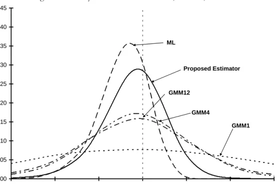
The results of running simulations with DGP A and DGP B are presented graphically in Figures 1 and 2. These figures plot smoothed density estimates, computed using a Gaussian kernel. In this and subsequent figures and tables, all estimates are normalized by dividing by the asymptotic standard error of the proposed estimator. The resulting quantities will asymptotically be distributed as N(0,v/v*), where v*=1.004 is the proposed estimator’s entry in line A of Table 2 and v is the corresponding value for the estimator in question (e.g., v=23.63 for GMM1).

Consistent with the asymptotic theory, Figures 1 and 2 make clear that our estimator is far more concentrated around 0 (the true parameter value) than are the conventional GMM

estimators. While it exhibits higher mean–and median–downward bias, it has dramatically lower variance and thus lower RMSE. Relative to our estimator, the ML estimator has larger bias and modestly lower RMSE.

The analogous plot for DGP C has densities that are very close to each other, so we do not include it. While our estimator performs better than the conventional GMM estimators in DGP C, it does so modestly. This result is consistent with Table 2, which showed that in DGP C the conventional GMM estimators are close to the proposed estimator in terms of asymptotic efficiency. As in DGPs A and B, ML has modestly lower RMSE than our estimator.

Table 3 presents summary statistics for all three DGPs and all four sample sizes. In columns (1) and (2), the table presents the median of 12 values (12 = 3 DGPs × 4 sample sizes) of RMSE and 12 values of median bias. (Column (3) will be discussed below.) Consistent with the figures just presented, the proposed estimator has distinctly lower RMSE than conventional GMM estimators, and modestly higher RMSE than ML.7 _{The same conclusion follows if one}

uses interquartile range rather than RMSE as the measure of variability (not reported in the table). In terms of median bias, our estimator is somewhat better than ML but somewhat worse than GMM1.

Figure 3 uses DGP A to illustrate how the quality of the asymptotic approximation of our estimator varies as the sample size T varies. The Figure shows that the asymptotic approximation

improves with T, and that there are notable departures from normality for all four values of T: for this DGP, even with T=10,000, our estimator still is a bit too variable. For DGP B (not shown), the asymptotic approximation looks good for T=10,000 and perhaps for T=1000 as well, while for DGP C we find little to complain about even for T=250.

We turn now from parameter estimation to hypothesis tests. Figures 4A, 4B and 4C present the actual size of two sided t-tests of H₀: $₁=0 for nominal sizes running from 0 to .25, for a sample size T=1000, for all three DGPs. The dashed line in each box is a 45 degree line; the other lines map nominal into actual size. Our proposed estimator is called “GMM*” in these figures. In all three DGPs, most lines are above the 45 degree dashed line, which means that the estimators tend to reject too much.8 _{The size distortions for the proposed estimator are always}

substantially less than those for GMM12 and somewhat less than those for ML, even though we use the simple variance-covariance estimator that is asymptotically valid only under correct specification (see the discussion below equation (2.4)). Unreported results indicate that the asymptotic approximation is better with larger sample sizes, with size distortions quite moderate when T=10,000, for all estimators. Column (3) of Table 3 presents a summary statistic, in the form of the median size across the 12 simulations of a nominal .10 test. The ideal value is of course 0.10. Our estimator’s value is 0.13, which means it performs slightly worse than GMM1 (median size =0.12), but modestly better than ML (median size =0.16).

Results are qualitatively similar for DGPs in which 0_t (defined in (4.1d)) was t- rather than normally distributed (not reported in a table). In particular, our estimator dominated other GMM estimators in terms of RMSE but not bias; QML generally had smaller RMSE and larger bias than did our estimator. One difference was that for T=250 or T=500 QML often had larger RMSE than did the proposed estimator. In terms of size, GMM1 was best, followed by our estimator and QML.

In summary, we see in these simulations that no estimator’s finite sample performance is perfectly, or even nearly perfectly, captured by the asymptotic approximation; as in many simulation studies of time series estimators, our simulations suggest that all available estimators

suffer from shortcomings of one sort or another. Further, and even apart from possible

inadequacy of the asymptotic approximation, rankings of estimators depend in part on measure of performance. Measures of bias favor conventional GMM estimators, especially GMM1;

measures of RMSE favor the proposed estimator or ML; measures of accuracy of test size favor GMM1 or the proposed estimator. Since the RMSEs of the conventional GMM estimators are considerably larger than those of the proposed estimator or ML, it is our sense that many researchers would turn to the proposed estimator or ML, even though the conventional GMM estimators have smaller bias and, in the case of GMM1, smaller size distortions as well. In terms of the simulation results, the trade off between the proposed estimator and ML is less sharp. Compared to the proposed estimator, ML is slightly better in terms of RMSE, slightly worse in terms of accuracy of hypothesis tests, somewhat worse in terms of bias.

Our simulations did not include the empirically interesting class of DGPs, such as those considered in Hayashi and Sims (1983), in which ML is inconsistent while our estimator is not. Hence these simulations probably make a conservative case for our estimator relative to ML. Thus we view our estimator as a reliable choice.

5. CONCLUSIONS

We have proposed and evaluated an instrumental variables estimator for linear models with conditionally heteroskedastic disturbances. The estimator is efficient in a class of estimators that are linear in a possibly infinite set of lags of a finite number of basic instruments. Implementation of the estimator requires specification of a parametric model. Simulations indicate that the

estimator often works well relative to a conventional estimator (Hansen (1982)) in common use, and comparably to maximum likelihood, even when the parametric model is misspecified. Priorities for future research include development and evaluation of efficient estimators that are nonlinear in lags of basic instruments, and alternative asymptotic approximations to better characterize the small sample distortions evident in many of the simulations.

1. Note that use of a vector AR or other model does not require knowledge of the entire set of structural equations relating the variables. This model is merely a device for computing

E(X_t|current and lagged z_t’s). See West and Wilcox (1996) for an illustration of this point in a conditionally homoskedastic environment.

2. One may of course omit the factor of F^2

e without changing the estimate of $. Note, however, one cannot then use (Q^N^S -1_Q^₎-1 _{to estimate the asymptotic variance-covariance}

matrix.

3. In finite samples, the present estimator and the West and Wilcox (1996) estimator will behave differently. As well, if conditional heteroskedasticity is absent, the West and Wilcox (1996) probably is computationally simpler than is the present estimator.

4. This last result may, however, be sensitive to the assumed form of heteroskedasticity (Broze et al. (2001)). Also, Stambaugh (1994) shows that fatter tails implies greater efficiency to use of additional lags.

5. That the disturbance ut impounds multiple shocks–in this case, two shocks,et and vt–is standard in rational expectations models in which private agents have more information than econometricians. It is the presence of multiple shocks that precludes conventional GLS filtering in such models.

6. Across all simulations we performed, about 1% of QML procedure runs did not converge when T=250, about 0.4% when T=500, and about 0.3% when T=1000. When T=10,000, there are only a handful of cases of non-convergence.

7. Note that we report root MSE here, while Table 2 reports variances. Table 3 indicates that the median value of MSE for GMM1 was about 3 times that of the proposed estimator [i.e., (1.92)2 _.3×(1.12)2_{], a value consistent with the median value of 3.73 in the GMM1 column in}

Table 2. Also, poor performance of a conventional estimator that relies on many lags as instruments (GMM12, in Table 3) is also found in Tauchen (1986) and West and Wilcox (1996).

8. Using the usual formula for the standard error of our coverage ratios, [p(1-p)/5000]½_{, where}

5000=number of repetitions, we have a standard error of about 0.003 for p=.05, of about 0.004 for p=.10. Some of the patterns just noted might therefore be due to sampling error in the simulations.

APPENDIX

Estimation of multiple equation systems proceeds as follows. Consider an R equation system, y_t=X_tN$+u_t, where y_t and u_t are (R×1), X_t is (k×R) and $ is (k×1). The (r×1) vector of basic instruments z_t has an (r×1) vector of innovations e_t that satisfies E(u_tqe_t-j)=0 for all j$0. Define e(t) = (1,e_tN,...,e_t-T+1N)N, ~e(t) = I_Rqe(t), S = Gq i=-qE[ut-iqe(t-i)][utNqe(t)N], (1+Tr)×1 (1+Tr)R×R (1+Tr)R× (1+Tr)R Q = EX_tNqe(t), G=S-1_Q. (1+Tr)R×k (1+Tr)R×k

Define ^e_t-j/0 for t-j<0, and otherwise use a “^” to denote a sample counterpart constructed by evaluating the indicated random variable or matrix of parameters at ^b. Then the optimal (k×R) instrument is Z^_t=G^N~^_{e(t), G}^_/^_S-1_Q^_{, with corresponding estimate $}^ _{= (E}T

t=1 ^ Z_tX_tN)-1_(ET t=1 ^ Z_ty_t).

Anatolyev, Stanislav, 2002, “Approximately Optimal Instrument for Multiperiod Conditional Moment Restrictions,” Working Paper, New Economic School.

Anatolyev, Stanislav, 2003, “The Form of the Optimal Nonlinear Instrument for Multiperiod Conditional Moment Restrictions,” Econometric Theory 19, 602-609.

Anatolyev, Stanislav, 2005, “GMM, GEL, serial correlation and asymptotic bias,” Econometrica 73, 983-1002.

Andrews, Donald W. K., 1991, “Heteroskedasticity and Autocorrelation Consistent Covariance Matrix Estimation,” Econometrica 59, 817-858.

Andrews, Donald W. K., 1999, “Consistent Moment Selection for Generalized Method of Moment Estimation,” Econometrica 67, 543-564.

Ang, Andrew, Geert Bekaert and Min Wei, 2006, “Do Macro Variables, Asset Markets, or Surveys Forecast Inflation Better?,” working paper, Columbia University.

Bates, Charles E. and Halbert White, 1993, “Determination of Estimators with Minimum Asymptotic Covariance Matrices,” Econometric Theory 9, 633-48.

Bollerslev, Tim, 1986, “Generalized Autoregressive Conditional Heteroskedasticity,” Journal of Econometrics 31 302-327.

Bollerslev, Tim, and Jeffrey M. Wooldridge, 1992, “Quasi Maximum Likelihood Estimation and Inference in Dynamic Models With Time Varying Covariances,” Econometric Reviews 11, 143-172.

Boudoukh, Jacob, Matthew Richardson, Robert Whitelaw, 2005, “The Myth of Long Horizon Predictability,” NBER Working Paper No. 11841.

Brown, Bryan W. and Shlomo Maital, 1981, “What Do Economists Know? An Empirical Study of Experts’ Expectations,” Econometrica 49, 491-504.

Broze, Laurence, Francq, Christian and Jean-Michel Zakoïan, 2001, “Non-redundancy of High Order Moment Conditions for Efficient GMM Estimation of Weak AR Processes,” Economics Letters 71, 317-322.

Breusch, Trevor, Qian, Hialong, Schmidt, Peter, and Donald Wyhowski, 1999, “Redundancy of Moment Conditions,” Journal of Econometrics 91, 89-111.

Carrasco, Raquel, Jose M. Labeaga and J. David Lopez-Salido, 2005, “Consumption and Habits: Evidence from Panel Data,” Economic Journal 115, 144-165.

Chinn, Menzie, 2006, “The (Partial) Rehabilitation of Interest Rate Parity in the Floating Rate Era: Longer Horizons, Alternative Expectations, and Emerging Markets,” Journal of International Money and Finance 26, 7-21.

Cragg, John G., 1983, “More Efficient Estimation in the Presence of Heteroskedasticity of Unknown Form,” Econometrica 51, 751-63.

den Haan, Wouter and Andrew Levin, 1996, “Inferences from Parametric and Non-Parametric Covariance Matrix Estimators,” National Bureau of Economic Research Technical Working Paper

Fama, Eugene F. and Kenneth R. French, 1988, “Permanent and Temporary Components of Stock Prices,” Journal of Political Economy 96, 246-73.

Fuhrer, Jeffery, 2006, “Intrinsic and Inherited Inflation Persistence,” International Journal of Central Banking 2, 49-86.

Hall, Alistair R. and Fernanda P.M. Peixe, 2003, “A Consistent Method for the Selection of Relevant Instruments,” Econometric Reviews 22, 269-287.

Hall, Robert E., 1988, “Intertemporal Substitution in Consumption,” Journal of Political Economy 96, 339-357.

Hansen, Bruce, 1994, “Autoregressive conditional density estimation,” International Economic Review 35, 705-730.

Hansen, Lars Peter, 1982, “Large Sample Properties of Generalized Method of Moments Estimators,” Econometrica 50, 1029-54.

Hansen, Lars Peter, 1985, “A Method for Calculating Bounds on the Asymptotic

Variance-Covariance Matrices of Generalized Method of Moments Estimators,” Journal of Econometrics 30, 203-228.

Hansen, Lars Peter, 1986, “Asymptotic Covariance Matrix Bounds for Instrumental Variables Estimators of Linear Time Series Models,” manuscript, University of Chicago.

Hansen, Lars Peter, Heaton, John C. and Masao Ogaki, 1988, “Efficiency Bounds Implied by Multiperiod Conditional Moment Restrictions,” Journal of the American Statistical Association 83, 863-871.

Hansen, Lars Peter, and Thomas J. Sargent, 1980, “Formulating and Estimating Dynamic Linear Rational Expectations Models,” Journal of Economic Dynamics and Control 2, 7-46.

Hansen, Lars Peter and Kenneth J. Singleton, 1991, “Computing Semi-Parametric Efficiency Bounds for Linear Time Series Models,” 387-412 in Barnett, W., Powell, J. and G. Tauchen (eds), Nonparametric and Semiparametric Methods in Econometrics and Statistics, Cambridge: Cambridge University Press.

Hansen, Lars Peter and Kenneth J. Singleton, 1996, “Efficient Estimation of Linear Asset Pricing Models with Moving-Average Errors,” Journal of Business and Economic Statistics 14, 53-68. Hayashi, Fumio and Christopher A. Sims, 1983, “Nearly Efficient Estimation of Time Series Models with Predetermined, but not Exogenous, Instruments", Econometrica 51, 783-798, Heaton, John C. and Masao Ogaki, 1991, “Efficiency Bounds for a Time Series Model With Conditional Heteroskedasticity,” Economics Letters 35, 167-171.

Hodrick, Robert J., 1987, The Empirical Evidence on the Efficiency of Forward and Futures Foreign Exchange Markets, Harwood Academic Publishers: New York.

Koenker, Roger and José A. F. Machado, 1999, “GMM Inference When the Number of Moment Conditions is Large,” Journal of Econometrics 93, 327-344.

Newey, Whitney K., 1988, “Adaptive Estimation of Regression Models via Moment Restrictions,” Journal of Econometrics 38, 301-339.

Newey, Whitney K. and Kenneth D. West, 1994, “Automatic Lag Selection in Covariance Matrix Estimation,” Review of Economic Studies 61 (1994), 631-654.

Parker, Jonathan A. and Christian Julliard, 2005, “Consumption Risk and the Cross Section of Expected Returns,” Journal of Political Economy 113, 185-222.

Ramey, Valerie A, 1991, “Nonconvex Costs and the Behavior of Inventories,” Journal of Political Economy 99, 306-34.

Renault, Eric and Bas J.M. Werker, 2006, “Causality Effects in Return Volatility Measures with Random Times,” manuscript, Tilburg University.

Schwert, G. William, 1989, “Why Does Stock Market Volatility Change over Time?,” Journal of Finance 44, 1115-53.

Shapiro, Matthew D., 1986, “The Dynamic Demand for Capital and Labor,” The Quarterly Journal of Economics 101, 513-542.

Stambaugh, Robert F., 1994, “Estimating Conditional Expectations When Volatility Fluctuates,” NBER Technical Working Paper No. 140.

Tauchen, George, 1986, “Statistical Properties of Generalized Method-of-Moments Estimators of Structural Parameters Obtained from Financial Market Data,” Journal of Business and Economic Statistics 4, 397-416.

West, Kenneth D., 1986, “Full Versus Limited Information Estimation of a Rational Expectations Model: Some Numerical Comparisons,” Journal of Econometrics 33, 367-386.

West, Kenneth D., 2001, “On Optimal Instrumental Variables Estimation of Stationary Time Series Models,” International Economic Review 42, 1043-1050.

West, Kenneth D., 2002, “Efficient GMM Estimation of Weak AR Processes,” Economics Letters 75, 415-418.

West, Kenneth D. and David W. Wilcox, 1994, “Estimation and Inference in the

Linear-Quadratic Inventory Model,” Journal of Economics Dynamics and Control 18, 897-908. West, Kenneth D. and David W. Wilcox, 1996, “A Comparison of Alternative Instrumental Variables Estimators of a Dynamic Linear Model,” Journal of Business and Economic Statistics 14, 281-293.

Zhang, Qiang and Masao Ogaki, 2004, “Decreasing Relative Risk Aversion, Risk Sharing and the Permanent Income Hypothesis,” Journal of Business and Economic Statistics 22, 421-430.

Asymptotic Variances Relative to Optimal GMM, ut=et+2-2et+1 N 2 ( (1 GMM1 GMM4 GMM12 ML 1. .9 0. .9 .1 1.00 1.00 1.00 0.88 2. .5 -.5 .9 .1 1.11 1.00 1.00 0.87 3. .5 .5 .9 .1 1.36 1.00 1.00 0.88 4. .5 .9 .9 .1 3.13 1.38 1.04 0.88 5. .5 .95 .9 .1 3.57 1.54 1.11 0.88 6. .9 .9 .9 .1 6.13 1.92 1.11 0.90 7. .9 .95 .0 .0 9.16 2.73 1.36 1.00 8. .9 .95 .5 .1 10.45 2.85 1.37 0.96 9. .9 .95 .9 .1 10.65 3.02 1.41 0.89 10. .9 1 .9 .1 9.92 2.88 1.38 n.a. 95 . Notes:

1. The model is y_t = $₀+z_t$₁+u_t, u_t = e_t+2-2e_t+1, z_t=Nz_t-1+e_t, e_t ~ GARCH(1,1), e_t=F_t0_t,0_t ~ iid(0,1), E04

t=3, F2t = T + (1e2t-1 + (2F2t-1, (/(1+(2. The figures are invariant to choice of T

(set to 0.1) and $₀ and $₁ (both set to zero).

2. GMMn is the conventional GMM estimator (Hansen (1982)) with a constant and lags 0 through

<