HAL Id: hal-01214840
https://hal.archives-ouvertes.fr/hal-01214840v4
Submitted on 7 Jul 2017HAL is a multi-disciplinary open access archive for the deposit and dissemination of sci-entific research documents, whether they are pub-lished or not. The documents may come from teaching and research institutions in France or abroad, or from public or private research centers.
L’archive ouverte pluridisciplinaire HAL, est destinée au dépôt et à la diffusion de documents scientifiques de niveau recherche, publiés ou non, émanant des établissements d’enseignement et de recherche français ou étrangers, des laboratoires publics ou privés.
Coupling Importance Sampling and Multilevel Monte
Carlo using Sample Average Approximation
Ahmed Kebaier, Jérôme Lelong
To cite this version:
Ahmed Kebaier, Jérôme Lelong. Coupling Importance Sampling and Multilevel Monte Carlo using Sample Average Approximation. Methodology and Computing in Applied Probability, Springer Verlag, 2018, 20 (2), pp.611-641. �10.1007/s11009-017-9579-y�. �hal-01214840v4�
Coupling Importance Sampling and Multilevel Monte Carlo
using Sample Average Approximation
Ahmed Kebaier∗& Jérôme Lelong† July 7, 2017
Abstract
In this work, we propose a smart idea to couple importance sampling and Multilevel Monte Carlo (MLMC). We advocate a per level approach with as many importance sam-pling parameters as the number of levels, which enables us to handle the different levels independently. The search for parameters is carried out using sample average approxi-mation, which basically consists in applying deterministic optimisation techniques to a Monte Carlo approximation rather than resorting to stochastic approximation. Our inno-vative estimator leads to a robust and efficient procedure reducing both the discretization error (the bias) and the variance for a given computational effort. In the setting of dis-cretized diffusions, we prove that our estimator satisfies a strong law of large numbers and a central limit theorem with optimal limiting variance, in the sense that this is the variance achieved by the best importance sampling measure (among the class of changes we consider), which is however non tractable. Finally, we illustrate the efficiency of our method on several numerical challenges coming from quantitative finance and show that it outperforms the standard MLMC estimator.
AMS 2000 Mathematics Subject Classification. 60F05, 62F12, 65C05, 60H35. Key Words and Phrases. Sample average approximation; multilevel Monte Carlo; vari-ance reduction; uniform strong large law of numbers; central limit theorem; importvari-ance Sampling.
1
Introduction
Expectations involving a stochastic process are often computed using a Monte Carlo method combined with a discretization scheme. For instance, computing a hedging portfolio in finance uses these tools. Generally, the asset price is modeled by a diffusion process(Xt)0≤t≤T, defined
as the solution of a stochastic differential equation (SDE)
dXt=b(Xt)dt+σ(Xt)dWt, X0=x∈Rd (1.1)
whereb:Rd→ Rd, σ :Rd → Md×q and W is a Brownian motion with values in Rq defined
on some given probability space(Ω,(Ft)0≤t≤T,P)with finite time horizonT >0. The process
∗
Université Paris 13, Sorbonne Paris Cité, LAGA, CNRS (UMR 7539), [email protected]. This research benefited from the support of the chair Risques Financiers, Fondation du Risque and the Laboratory of Excellence MME-DII (http://labex-mme-dii.u-cergy.fr/).
†
X hardly ever has an explicit solution, which implies that its simulation requires the use of a discretization scheme. For n ∈N∗, consider the continuous time Euler approximation Xn
with time step δ =T /n given by
dXtn=b(Xηnn(t))dt+σ(Xηnn(t))dWt, ηn(t) =bt/δcδ.
This work aims at combining importance sampling with different discretization methods: first, we study the use of importance sampling for the standard case of Euler Monte Carlo and then we apply it to MLMC. Many different changes of measure can be used to implement importance sampling. When working with Lévy processes, it is common to use the Esscher transform to introduce a new family of measures. For Brownian driven SDEs, the Esscher transform actually corresponds to a Gaussian change of measure in the spirit of the Girsanov theorem. Following the ideas of Arouna [1], we consider a parametric family of stochastic processes (Xt(θ))0≤t≤T, withθ∈Rq, driven by a Brownian motion with linear drift
dXt(θ) = (b(Xt(θ)) +σ(Xt(θ))θ)dt+σ(Xt(θ))dWt.
We also define the continuous time Euler approximation Xn(θ) of the process X(θ). From Girsanov’s Theorem, the process (Btθ =∆ Wt+θt)t≤T is a Brownian motion under the new
probability measure Pθ equivalent to Pand such that
dPθ dP|Ft = exp −θ·Wt− 1 2|θ| 2t ∆ =E−(W, θ). Therefore, EP[ψ(XT)] =EPθ[ψ(XT(θ))] =EP ψ(XT(θ))E−(W, θ) . (1.2)
This equality still holds when replacingX(resp. X(θ)) by its Euler schemeXn(resp. Xn(θ)).
The l.h.s. and r.h.s. expectations are both computed under the original probability measure. In the following, we will always use the measurePand therefore we will not write it anymore. The idea of importance sampling Monte Carlo is to use the r.h.s of (1.2) to build a Monte Carlo estimator ofE[ψ(XT)] usingXn(θ) withθgiven by
θ? = argmin
θ∈Rq
Var ψ(XT(θ))E−(W, θ)
.
Importance sampling for Euler Monte Carlo is studied in Section 2: first, we investigate how to approximateθ? in practice and second we prove that the Monte Carlo estimator combined with this approximation of θ? satisfies a strong law of large numbers and a central limit theorem when both n and the number of samples go to infinity. This result extends the limit theorems obtained in [23], in which the authors investigated the case of a fixed number of discretization steps n. The error induced by using E[ψ(XTn(θ))] instead of E[ψ(XT(θ))]
is called the discretization error and is responsible for the bias of the Euler Monte Carlo estimator, while the Monte Carlo approximation only impacts the variance. The two errors are balanced when the number of samples N of the Monte Carlo method is proportional to n2, which leads to an overall complexity of order n3. In order to reduce the bias for a given computational effort, Kebaier [24] proposed to use the Statistical Romberg method, which combines discretization schemes on two nested time grids. This method was generalized
by Giles [13] who proposed to use a multilevel Monte Carlo algorithm following the line of Heinrich’s multilevel method for parametric integration [19].
Let m, L ∈ N with m ≥ 2 and L > 0, the idea of the multilevel method is to write the expectation on the finest time grid as a telescopic sum involving all the other grids (referred to as levels) E[ψ(Xm L T )] =E[ψ(Xm 0 T )] + L X `=1 E[ψ(Xm ` T )−ψ(Xm `−1 T )] (1.3)
and then to approximate each expectation by a Monte Carlo method with a well chosen number of samples to balance the errors between the different terms. We refer the reader to the extensive literature on MLMC for more details, see e.g. [3, 9, 10, 11, 14, 16, 15, 18, 20, 27]. For a fixed computational budget, the use of multilevel techniques clearly reduces the bias, but in many situations the high variance also brings in a significant inaccuracy, which naturally leads to trying to couple MLMC with variance reduction techniques.
In this work, we focus on coupling importance sampling with MLMC. In [5] and [17], the authors choose to apply MLMC to the right hand side of (1.2) coming up with
E[ψ(Xm L T )] =E h ψ(XTm0(λ))E−(W, λ)i + L X `=1 E h (ψ(XTm`(λ))−ψ(XTm`−1(λ)))E−(W, λ)i. (1.4)
This approach mixes all the levels through the optimization of the parameter λ and breaks the independence between the levels of the multilevel approach, which nonetheless made it so popular and easy to implement.
Instead of using (1.4), we would rather apply importance sampling to each expectation in the telescopic sum of (1.3) to obtain forλ1, . . . , λL∈Rq
E[ψ(Xm L T )] =E h ψ(XTm0(λ0))E−(W, λ0) i + L X `=1 E h (ψ(XTm`(λ`))−ψ(Xm `−1 T (λ`)))E−(W, λ`) i .
Our importance sampling multilevel estimator is obtained by applying a Monte Carlo method to each of the levels`withN` samples
QL(λ0, . . . , λL) = 1 N0 N0 X k=1 ψ( ˜XT,m00,k(λ0))E−( ˜W0,k, λ0) + L X `=1 1 N` N` X k=1 ψ( ˜XT ,`,km` (λ`))−ψ( ˜Xm `−1 T ,`,k (λ`)) E−( ˜W`,k, λ`) (1.5)
The samples used in the different levels are independent and within each level they are i.i.d. For any `≥0, the variables X˜T ,`,km` (λ`) (resp. X˜m
`−1
T ,`,k (λ`) when` >0) are the terminal values
of the Euler schemes ofX(λ`)withm`(resp. m`−1) time steps built using the same Brownian
pathW˜`,k. The variance of the importance sampling MLMC estimator is given by
Var[Q ] =N−1σ (λ )2+
L
X
where σ02(λ0) ∆ = Var[ψ(XTm0(λ0))E−(W, λ0)] σ2`(λ`) ∆ = m ` (m−1)TVar h ψ(XTm`(λ`))−ψ(Xm `−1 T (λ`)) E−(W, λ`) i .
By allowing for one importance sampling parameterλ` per level, our approach has many
ad-vantages over [5, 17]. First, the computations within the different levels remain independent. Second, the variance of each level` only depends on λ`, which reduces the global
minimiza-tion problem to several smaller minimizaminimiza-tion problems. Third, we actually minimize the real variance of the estimator and not its asymptotic value and more importantly it can be imple-mented without knowing∇ψ, which however appears in the central limit theorem for MLMC. The new idea of using one importance sampling parameter per level was later taken up in [6] but coupled with stochastic approximation to build adaptive estimators.
Actually, minimizing λ7−→σ2
`(λ) can be achieved by using the randomly truncated
Rob-bins Monro algorithm proposed by Chen et al. [7, 8] and later investigated in the context of importance sampling by Lapeyre and Lelong [25] and Lelong [26]. The numerical stability of these stochastic algorithms strongly depends on the choice of the descent step — often referred to as the gain sequence — which proves to be highly sensitive in practice. To overcome this difficulty, Jourdain and Lelong [23] proposed to apply deterministic optimization techniques to sample average estimators to search for the optimal parameter. Following their methodology, we defineσ2`,N0
`
as the sample average approximation ofσ`2withN`0 samples using the standard empirical Monte Carlo estimator of the variance. We assume that the samples used in σ`,N2 0
`
are independent of those used inQL. We refer to Section 3 for more details on how to choose
the samples in the different approximations. Now, we sketch the algorithm corresponding to our method.
1 for`= 0 :Ldo
2 Sample the random functionλ7−→σ`,N0
`(λ). // σ
2
`,N0
` is the sample average
approximation of σ`2, see Section 3.1
3 Computeλˆ`= argminσ`,N2 0
`
(λ) using Newton–Raphson’s algorithm. 4 Independently ofσ`,N2 0
`
, sample the level `of (1.5) usingλˆ`.
5 end
6 Sum all the levels to obtain
QL(ˆλ0, . . . ,ˆλL) = 1 N0 N0 X k=1 ψ( ˜XT ,m00,k(ˆλ0))E−( ˜W0,k,ˆλ0) + L X `=1 1 N` N` X k=1 ψ( ˜XT ,`,km` (ˆλ`))−ψ( ˜Xm `−1 T ,`,k (ˆλ`)) E−( ˜W`,k,ˆλ`).
Algorithm 1.1: Multilevel Importance Sampling (MLIS)
First, we investigate in Section 2 the standard Euler Monte Carlo method coupled with importance sampling. Then, in Section 3, we study the importance sampling framework with
MLMC. We prove thatQL(ˆλ0, . . . ,λˆL) satisfies a strong law of large numbers and a central
limit theorem. Our MLIS estimator achieves the smallest possible variance within the family of MLMC estimators approximating E[ψ(XT)] using the class of processes(X(λ))λ∈Rq. Note
that this is also the limiting variance obtained in [5] for the MLMC estimator built on (1.4) with the best possible parameterλ∈ Rq. The main difficulty in proving these results is the
uniform control of the triangular arrays involved in the adaptive multilevel estimator. To overcome this issue, we prove in Section 4 new limit theorems for doubly indexed sequences of random variables in a general setting (see Propositions 4.1 and 4.3). In section 5, we illustrate the efficiency of MLIS on challenging problems coming from quantitative finance and show that it outperforms the standard MLMC estimator.
2
Importance sampling with Euler Monte Carlo
2.1 Notation and general assumptions
• For a vector x∈Rq,|x|denotes the Euclidean norm ofx.
• The superscript ∗ denotes the transpose operator.
• For a matrix A ∈ Md×q,|M| denotes the Frobenius norm ofA defined by
p
Tr(A∗A), which corresponds to the Euclidean norm onRd×q.
• For q∈N∗,Iq denotes the identity matrix with size q×q.
• For α >0, we define the set of functions
Hα=nψ:Rd→Rs.t. ∃c >0, β≥1, ∀x∈Rd, |ψ(x)| ≤c(1 +|x|β)
and∀x, y∈Rd, |ψ(x)−ψ(y)| ≤c(1 + (|x|β∧ |y|β))|x−y|α
o
(2.1)
• For a sequence of random variables (Xn)n, “Xn=⇒X” means that(Xn)n converges in
distribution to X.
Here, we gather several standard assumptions required to ensure the convergence of the Euler scheme.
(H-1) i. The functionsb andσ are Lipschitz
∀x, y∈Rd, |b(x)−b(y)|+|σ(x)−σ(y)| ≤Cb,σ|x−y|, (Hb,σ)
for some real numberCb,σ >0.
ii. ∀p≥1, X, Xn∈Lp and there existsKp(T)>0s.t.
E " sup 0≤t≤T |Xt−Xtn| p # ≤ Kp(T) np/2 .
iii. There existγ ∈[1/2,1]and Cψ(T, γ)>0 s.t.
nγ(Eψ(XTn)−Eψ(XT))→Cψ(T, γ). (Hγ)
2.2 General framework
In this section, we investigate the case of an Euler Monte Carlo approach. We consider the importance sampling representation ofE[ψ(XT)]given by
E[ψ(XT(θ))E−(W, θ)].
The optimal value forθis given by
θ? = argmin
θ∈Rq
with v(θ)=∆E[(ψ(XT(θ))E−(W, θ))2].
By using (1.2), we can rewritev as
v(θ) =E[ψ(XT)2E+(W, θ)] with E+(W, θ)
∆
= e−WT·θ+|θ2|.
From a practical point of view, the quantity v(θ) is not explicit so we use the Euler scheme to discretizeX(θ) and approximate θ? by
θn ∆ = argmin θ∈Rq vn(θ) with vn(θ) ∆ =Eψ(XTn)2E(W, θ) . (2.3)
Since the expectation is usually not tractable, we replace it by its sample average approxima-tion and define
θn,N ∆ = argmin θ∈Rq vn,N(θ) with vn,N(θ) ∆ = 1 N N X i=1 ψ(XT ,in )2E(Wi, θ) , (2.4)
where (XT ,in , WT ,i)1≤i≤N are i.i.d. samples with the law of (XTn, WT). The existence and
uniqueness of θ?,θn and θn,N are ensured by the following lemma whose proof can easily be
adapted from [23, Lemma 1.1].
Lemma 2.1. Under Condition (H-2), the functionsv, vnandvn,N are infinitely continuously
differentiable for all n, N and the derivatives are obtained by exchanging expectation and dif-ferentiation. Moreover, the functions v and vn are strongly convex and so is vn,N for any N
such that vn,N is not identically zero.
2.3 Convergence of the optimal importance sampling parameter
Theorem 2.2. Suppose σ and b satisfy (Hb,σ). Let ψ satisfy Condition (H-2) and belong to
Hα for someα >0. Then, θn→θ? a.s. when n→+∞.
By Hölder’s inequality, for any functionψ∈ Hα, (H-2) implies thatsupnE[ψ(XTn)2e
−θ·WT]<
+∞. Hence, the proof of the theorem ensues from [5, Theorem 2.2].
In the following, we letN depend onn so thatN =∆ Nn tends to infinity withn.
Proposition 2.3. Assume that Assumption (Hb,σ) holds and that ψ ∈ Hα for some α > 0. Then, for allK >0, a.s. when n→ ∞
sup
|θ|≤K
|vn,Nn(θ)−v(θ)| →0; sup
|θ|≤K
Proof. The proof of the two results are very similar, we omit the second one and concentrate on the uniform convergence forvn,Nn. To do so, we will apply Proposition 4.3. Now, we check
Assumptions (H-4), (H-5), (H-6). At first, note that under Assumption (Hb,σ), we have the almost sure convergence of XTn towards XT. As ψ ∈ Hα, it follows from Property (H-1)-ii
that for alla >1, supn∈NE
h ψ(X n T)2e −θ·WT+12|θ| 2T ai
<∞. Note that for every fixedn, the sequence
ψ(XT ,in )2e−θ·WT ,i+12|θ| 2T
i is i.i.d. Then, we deduce that for allm∈N ∗ lim n→∞E[vn,m(θ)] =E h ψ(XT)2e−θ·WT+ 1 2|θ| 2Ti .
This yields (H-4). Let K > 0. As ψ ∈ Hα we obtain using the Cauchy Schwarz inequality
and Property (H-1)-ii that
sup n sup m mVar sup |θ|≤K vn,m(θ) ! ≤sup n E 1/2 ψ(XTn)8E1/2 " sup |θ|≤K e−4θ·WT+2|θ|2T # <∞.
Using the same arguments, we also get
sup n sup m Var ψ(XT ,mn )2 sup |θ|≤K e−θ·WT ,m+12|θ|2T ! <∞.
This yields (H-5). Concerning the last assumption, if we fixδ >0,θ∈Rd and setB(θ, δ) —
the open ball with centerθand radius δ — then the Cauchy Schwarz inequality gives
sup n E " ψ(XTn)2 sup θ0∈B(θ,δ) e −θ0·WT+12|θ 0|2T −e−θ·WT+12|θ| 2T #2 ≤ sup n E ψ(XTn)4 E " sup θ0∈B(θ,δ) e −θ0·WT+12|θ 0|2T −e−θ·WT+12|θ| 2T 2# .
Using the elementary inequality|ex−ey| ≤ |x−y|(ex+ ey), we easily deduce that the quan-tityE supθ0∈B(θ,δ) e −θ0·WT+12|θ0|2T −e−θ·WT+12|θ|2T 2
can be made arbitrarily small. Finally, Assumption (H-6) is satisfied using Remark 4.4.
Theorem 2.4. Assume that Assumption (Hb,σ) holds and that ψ ∈ Hα for some α > 0. Then, θn,Nn −→θ ? a.s. and √N n(θn,Nn−θ ?) =⇒N(0,Γ) whenn→ ∞ with Γ = [∇2v(θ?)]−1Var(T θ?−W T)ψ(XT)2e−θ ?·W T+12|θ ?|2T [∇2v(θ?)]−1.
Proof. We already know from Proposition 2.3 that a.s. vn,Nn converges locally uniformly to
v. Let ε >0. By the strict convexity ofv,δ= inf∆ |θ−θ?|≥εv(θ)−v(θ?)>0.
The local uniform convergence ofvn,Nn to v ensures that
∃nδ>0,∀n≥nδ,∀θ∈Rq s.t. |θ−θ?| ≤ε, |vn,Nn(θ)−v(θ)| ≤
δ
Forn≥nδ and θ such that|θ−θ?| ≥ε, we can deduce from the convexity of vn,Nn that vn,Nn(θ)−vn,Nn(θ ?)≥ |θ−θ?| ε vn,Nn θ?+ε θ−θ ? |θ−θ?| −vn,Nn(θ ?) ≥ |θ−θ ?| ε v θ?+ε θ−θ ? |θ−θ?| −v(θ?)−2δ 3 ≥ δ 3
where the last two inequalities come from (2.5). If we apply this inequality for θ = θn,Nn,
we obtain a contradiction since vn,Nn(θn,Nn)−vn,Nn(θ
?) ≤ 0. Hence, we deduce that for all n ≥ nδ, |θn,Nn −θ
?| < ε. Therefore, θ
n,Nn converges a.s. to θ
?. If we combine this result
with the local uniform convergence of vn,Nn to the continuous function v, we deduce that
vn,Nn(θn,Nn) converges a.s. tov(θ
?).
Moreover, we get by Equation (3.9) that for allK >0 sup |θ|≤K ∂θ(j)ψ(XT) 2e−θ·WT+12|θ|2T ≤eK2T /2ψ(XT)2 K+ (eKWt(j) + e−KW (j) t ) Yq i=1 (eKWt(i)+ e−KW (i) t ).
The r.h.s is integrable by Condition (H-2). Hence, Ehsup|θ|≤K
∇θψ(XT) 2e−θ·WT+12|θ| 2T i <
+∞. Similarly, one can prove thatEhsup|θ|≤K
∇ 2 θψ(XT)2e −θ·WT+12|θ|2T i < +∞. Then, to prove the central limit theorem governing the convergence of θn,Nn to θ
?, we reproduce the
proof of [29, Theorem A2, pp. 74], which is mainly based on the a.s. local uniform convergence of∇vn,Nn and on its asymptotic normality ensuing from Theorem A.1.
2.4 A second stage Monte Carlo approach
In this section, we aim at building adaptive Monte Carlo estimators in the setting of discretized diffusion processes following the spirit of [23]. Our setting differs mainly because we want to let both the number of time steps and the number of samples go to infinity. Asymptotic results rely on a uniform control of the triangular arrays involved in the adaptive importance sampling Monte Carlo estimator. The technical results from Section 4 will be tremendously useful to provide such controls.
Using the estimators of θ? studied in the previous section, we define a Monte Carlo esti-mator ofE[ψ(XT)]based on Equation (1.2). We introduce the σ-algebra G generated by the
samples(Wi)i≥1 used to computeθn andθn,Nn.
Let( ˜Wi)ibe i.i.d. samples according to the law ofW but independent ofG. Conditionally
on G, we introduce i.i.d. samples ( ˜Xi(θn,Nn))i following the law of X(θn,Nn) such that for
eachi,X˜i(θn,Nn)is the solution of the SDE driven byW˜i. We introduce( ˜Gk)k>0 the filtration
defined byG˜k=σ( ˜Wi,1≤i≤k)andGk] =G ∨G˜k. For eachi >0, we also considerX˜in(θn,Nn)
defined as the Euler discretization ofX˜i(θn,Nn). Based on these new sets of samples, we define
Mn,Nn = 1 Nn Nn X i=1 g(θn,Nn,X˜ n T,i(θn,Nn),W˜T,i),
where the functiong:Rq×Rd×Rq→Ris defined by
g(θ, x, y)=∆ψ(x)e−θ·y−12|θ| 2T
For the clearness of the coming proofs, it is convenient to introduce the following notation Mn,Nn(θ) = 1 Nn Nn X i=1 g(θ,X˜T ,in (θ),W˜T ,i). Note that Mn,Nn =Mn,Nn(θn,Nn).
Theorem 2.5. Assume that Assumption (Hb,σ) holds and that ψ ∈ Hα for some α > 0. Then, Mn,Nn −→E[ψ(XT)] a.s. when n→+∞.
Proof. Using the conditional independence of the samples( ˜Xin(θn,Nn),W˜i)i, we have
E[g(θn,Nn,X˜ n T,i(θn,Nn),W˜T,i)|G] =E[ψ(X n T)] ∆ =en for alli >0.
Let V ⊂Rq be a compact neighbourhood ofθ?. We define the sequence
Yi,n= g(θn,Nn,X˜ n T ,i(θn,Nn),W˜T ,i)−en 1{θ n,Nn∈V}
and its empirical average Ym,n = m1 Pmi=1Yi,n for all m > 0. It is obvious that E[Yi,n] = 0
and using the conditional independenceE[Ym,n 2 ] = m1E[|Y1,n|2]. E[|Y1,n|2]≤E h E h |g(θn,Nn,X˜ n T,i(θn,Nn),W˜T,i)−en| 2 G i 1{θ n,Nn∈V} i ≤Ehvn(θn,Nn)1{θn,Nn∈V} i ≤sup θ∈V vn(θ).
We know thatvnis convex and converges point-wise tov, which is also convex and continuous.
Hence, vn converges locally uniformly to v, which implies that for all compact sets K ⊂Rq,
limn→+∞supθ∈Kvn(θ) = supθ∈Kv(θ). Hence, supnsupθ∈Vvn(θ) < +∞. Applying
Proposi-tion 4.1 proves thatYNn,n
a.s.
−−−−−→
n→+∞ 0. Asθn,Nn converges a.s. toθ
? ∈K, this also implies that
limn→+∞Mn,Nn =E[ψ(XT)]a.s.
Theorem 2.6. Under the assumptions of Theorem 2.5 and if Condition (Hγ)holds, we have
p Nn(Mn,Nn−E[ψ(XT)]) =⇒ N(Cψ(T, α), σ 2) when n→+∞. whereσ2 =E h ψ(XT)2e−θ ?·W T+12|θ?|2T i −E[ψ(XT)]2.
Remark 2.7. Assume the number of time steps used in the Euler scheme is fixed to n = 1
and consider the estimator M1,N(θ1,N). Then, we know from [2, Theorem 3.4] that, when N → ∞, M1,N(θ1,N)−→E[g(θ1, XT1(θ1), WT)] a.s. √ N(M1,N(θ1,N)−E[g(θ1, XT1(θ1), WT)]) =⇒ N(0, σ21) with σ2 1 =E h ψ(X1 T)2e −θ1·WT+12|θ1|2T i −E[ψ(XT1)]2.
Proof. We can write the left hand side of the convergence result by introducing Mn,Nn(θ ?) p Nn(Mn,Nn−E[ψ(XT)]) = p Nn(Mn,Nn(θn,Nn)−Mn(θ ?)) +p Nn(Mn,Nn(θ ?)− E[ψ(XT)])
The convergence of the last term on the r.h.s√Nn(Mn,Nn(θ
?)−
E[ψ(XT)])is governed by the
central limit theorem for Euler Monte Carlo, which yields the announced limit (see [12]). It remains to prove that√Nn(Mn,Nn(θn,Nn)−Mn,Nn(θ
?))converges to zero in probability.
Letε >0and α < 12, P p Nn|Mn,Nn(θn,Nn)−Mn,Nn(θ ?)|> ε = P p Nn|Mn,Nn(θn,Nn)−Mn,Nn(θ ?)|> ε; Nα n|θn,Nn−θ ?|>1 +P p Nn|Mn,Nn(θn,Nn)−Mn,Nn(θ ?)|> ε; Nα n|θn,Nn−θ ?| ≤1 = P(Nnα|θn,Nn−θ ?|>1) +P p Nn|Mn,Nn(θn,Nn)−Mn,Nn(θ ?)|1 {Nα n|θn,Nn−θ?|≤1}> ε . By Theorem 2.4,P(Nnα|θn,Nn−θ
?|>1)tends to zero whenngoes to infinity. LetK >0s.t.
for allnlarge enough {θ∈Rq : |θ−θ?| ≤N−α
n } ⊂B(0, K). We can bound the second term
on the r.h.s. by using Markov’s inequality
P p Nn|Mn,Nn(θn,Nn)−Mn,Nn(θ ?)|1 {Nα n|θn,Nn−θ?|≤1}> ε ≤ Nn ε2 E h |Mn,Nn(θn,Nn)−Mn,Nn(θ ?)|21 {θn,Nn∈B(0,K)} i ≤ 1 ε2E h |g(θn,Nn,X˜ n T(θn,Nn),W˜T)−g(θ ?,X˜n T(θ?),W˜T)|21{θn,Nn∈B(0,K)} i ≤ 1 ε2E h |g(θn,Nn,X˜ n T(θn,Nn),W˜T)−g(θn,Nn,X˜T(θn,Nn),W˜T)| 21 {θn,Nn∈B(0,K)} i + 1 ε2E h |g(θn,Nn,X˜T(θn,Nn) ˜WT)−g(θ ?,X˜n T(θ?),W˜T)|21{θn,Nn∈B(0,K)} i .
We treat each of the two terms separately.
I First term
From the independence betweenθn,Nn and W˜, we can write
E h |g(θn,Nn,X˜ n T(θn,Nn),W˜T)−g(θn,Nn,X˜T(θn,Nn),W˜T)| 21 {θn,Nn∈B(0,K)} i =E |ψ(XTn)−ψ(XT)|2exp(−θn,Nn·W˜T + 1 2|θn,Nn| 2T)1 {θn,Nn∈B(0,K)} ≤Eh|ψ(XTn)−ψ(XT)|2(1+η) i1+1η e 1+2η 2η K 2T , for some η >0.
Relying on the uniform integrability ensured by property (H-1)-ii and since ψ∈ Hα, we can letngo to infinity inside the expectation to obtain that
lim n→+∞E h |g(θn,Nn,X˜ n T(θn,Nn),W˜T)−g(θn,Nn,X˜T(θn,Nn),W˜T)| 21 {θn,Nn∈B(0,K)} i = 0. I Second term
Since the functiongis continuous w.r.t its first two parameters andXTθ is continuous w.r.t the parameterθ,limn→+∞g(θn,Nn,X˜T(θn,Nn),W˜T)−g(θ
?,X˜n
T(θ?),W˜T) = 0a.s. To conclude
the proof, we need to show that the family of r.v.
|g(θn,Nn,X˜T(θn,Nn),W˜T)−g(θ ?,X˜n T(θ?),W˜T)|21{θn,Nn∈B(0,K)} n is uniformly integrable.
First, for any θ∈Rq and 2(1 +η)> a >2
E h |g(θ,X˜T(θ),W˜T)|a i =E |ψ( ˜XT)|ae−(a−1)θ· ˜ WT+(a−1)|θ| 2T 2 ≤Eh|ψ( ˜XT)|2(1+η) i2(1+aη) eC|θ|2 (2.7)
whereC is a constant only depending onaand T. This yields that for some δ >0 and some constantC >0independent of θ,E h |g(θ,X˜T(θ),W˜T)|2+δ i < CeC|θ|2. Then, we get sup n E h |g(θn,Nn,X˜T(θn,Nn),W˜T)| 2+δ1 {θn,Nn∈B(0,K)} i = sup n E h E h |g(θn,Nn,X˜T(θn,Nn),W˜T)| 2+δ|θ n,Nn i 1{θ n,Nn∈B(0,K)} i ≤sup n CE h eC|θn,Nn|21 {θn,Nn∈B(0,K)} i ≤CeCK.
We can similarly obtain that
sup n E h |g(θ?,X˜Tn(θ?),W˜T)|2+δ i ≤sup n E h |ψ(XTn)|2(1+η)i 2(1+η) 2+δ eC|θ?|2.
This proves that the family of r.v.
|g(θn,Nn,X˜T(θn,Nn),W˜T)−g(θ ?,X˜n T(θ?),W˜T)|21{θn,Nn∈B(0,K)} n
is uniformly integrable, which ends the proof.
3
Multilevel Importance sampling Monte Carlo
In the recent years, many works showed that MLMC supersedes Monte Carlo when combined with discretization schemes. Then, it has become natural to investigate how this new approach could be coupled with existing variance reduction techniques and in particular with importance sampling. In this section, we study the mathematical properties of our importance sampling MLMC estimatorQL(ˆλ0, . . . ,λˆL). First, we start by proving the existence and uniqueness of
ˆ
λ0, . . . ,ˆλL in Section 3.2 and then we prove a strong law of large numbers and a central limit
3.1 General framework
Our multilevel importance sampling estimator writes
QL(λ0, . . . , λL) = 1 N0 N0 X k=1 ψ( ˜XT,m00,k(λ0))E−( ˜W0,k, λ0) + L X `=1 1 N` N` X k=1 ψ( ˜XT ,`,km` (λ`))−ψ( ˜Xm `−1 T ,`,k(λ`)) E−( ˜W`,k, λ`). (3.1)
For any fixed ` ∈ {1,· · · , L}, the random variables ( ˜W`,k)1≤k≤N` are independent and are
distributed according to the Brownian law. We assume that for`, `0 ∈ {1,· · ·, L}, with`6=`0, the blocks( ˜W`,k)1≤k≤N` and( ˜W`0,k)1≤k≤N`0 are independent. For any fixed`∈ {1,· · · , L}and
k∈ {1, . . . , N`}, the variablesX˜m
`
T ,`,k(λ`)(resp. X˜m
`−1
T ,`,k (λ`)) are the terminal values of the Euler
schemes ofX(λ`)withm` (resp. m`−1) time steps built using the same Brownian path W˜`,k.
The key of the multilevel approach is to use the same Brownian path to compute X˜m` T,`,k(λ`)
andX˜T ,`,km`−1(λ`). The blocks of random variables used in two different levels are independent.
From these assumptions, one can compute the variance of the multilevel estimator given by
Var[QL] =N0−1σ0(λ0)2+ L X `=1 N`−1(m−1)T m` σ 2 `(λ`) where σ02(λ0)= Var[∆ ψ(Xm 0 T (λ0))E−(W, λ0)] σ`2(λ`) ∆ = m ` (m−1)TVar hn ψ(XTm`(λ`))−ψ(Xm `−1 T (λ`)) o E−(W, λ`) i .
By applying (1.2), the variances of each level`≥0 can be writtenσ`2(λ`) =v`(λ`)−Ξ2` with
v0(λ0) ∆ =E h ψ(XTm0)2E+(W, λ 0) i , Ξ0 ∆ =E h ψ(XTm0)i (3.2) v`(λ`) ∆ = m ` (m−1)TE ψ(X m` T )−ψ(Xm `−1 T ) 2 E+(W, λ`) , (3.3) Ξ` ∆ = s m` (m−1)TE h ψ(XTm`)−ψ(XTm`−1) i (3.4)
andE+(W, λ)= e∆ −λ·WT+12|λ|2T.Hence, the global variance is given by
Var[QL] =N0−1(v0(λ0)−Ξ20) + L X `=1 N`−1(m−1)T m` v`(λ`)−Ξ 2 ` .
To actually minimize the functionsλ7−→v2`(λ), we consider the sample average approximation ofv` withN`0 samples v0,N0 0(λ0) ∆ = 1 N00 N00 X k=1 ψ(XT ,m00,k)2E+(W0,k, λ0), v`,N0 `(λ`) ∆ = 1 N`0 N`0 X k=1 m` (m−1)T ψ(X m` T,`,k)−ψ(Xm `−1 T ,`,k) 2 E+(W`,k, λ`).
3.2 Convergence of the importance sampling parameters
From Lemma 2.1, we deduce thatv`,N0
` has a unique minimum b
λ`= arg min λ∈Rqv`,N
0
`(λ).
Theorem 3.1. Assume b and σ are C1 with bounded derivatives, ψ ∈ Hα for some α ≥ 1, ψ isC1 and ∇ψ has polynomial growth. Then, the sequence of random functions(v`,N0
`:λ∈
Rq → v`,N0
`(λ))` converges a.s. locally uniformly to the strongly convex function v :R
q → R defined by v(λ)=∆E h (∇ψ(XT)·UT)2E+(W, λ) i (3.5) with dUt=∇b(Xt)Utdt+ q X j=1 ∇σj(Xt)UtdWtj− 1 √ 2 q X ij,=1 ∇σj(Xt)σi(Xt)dWˇti,j (3.6)
whereWˇ is a Brownian motion independent of W with values in Rq×q. Moreover,λb` converges a.s. to λ?
∆
= arg minλv(λ), when `→+∞.
Proof. Let us define the doubly indexed sequence
Yk,`(λ) = m` (m−1)T ψ(X m` T ,k)−ψ(Xm `−1 T ,k ) 2 E+(Wk, λ).
For any fixed`, the sequence(Yk,`(λ))k is i.i.d. so that for anyk,E[Yk,`(λ)] =y`(λ) with
y`(λ) =E m` (m−1)T ψ(X m` T )−ψ(Xm `−1 T ) 2 E+(W, λ) .
We deduce from Proposition A.4 that the sequence (y`)` converges pointwise to the
contin-uous function E
h
(∇ψ(XT)·UT)2E+(W, λ)
i
, thus satisfying Assumption (H-4)-i. The i.i.d. property of the sequence(Yk,`(λ))k also implies that
E sup |λ|≤K 1 N N X k=1 Yk,`(λ) !2 ≤E " 1 N N X k=1 sup |λ|≤K Yk,`(λ)2 # ≤ 1 NE " sup |λ|≤K Y1,`(λ)2 # . (3.7)
E " sup |λ|≤K Y1,`(λ)2 #2 ≤E " m` (m−1)T ψ(X m` T )−ψ(Xm `−1 T ) 24# E " sup |λ|≤K E+(W, λ)4 # . (3.8)
Using the following upper bound
sup |λ|≤K e−λ·WT+12|λ| 2T ≤e12K 2T q Y l=1 (eKWT(l)+ e−KW (l) T ), (3.9) E h sup|λ|≤KE+(W, λ)4 i
< +∞. Let us have a closer look at the first term in (3.8). From Condition (2.1), we can write
E " m` ψ(X m` T )−ψ(Xm `−1 T ) 24# ≤CE m4` X m` T −Xm `−1 T 8α 1 + X m` T 8β + X m`−1 T 8β .
By using the strong rate of convergence of the Euler scheme, we notice that for anyp >1,
E m4`p X m` T −Xm `−1 T 8αp ≤m4`pC m−4αp`+m−4αp(`−1) ≤Cm4αp−4`p(α−1).
Hence, sinceα≥1, by using the Cauchy Schwartz inequality we easily check that
sup ` E " m` (m−1)T ψ(X m` T )−ψ(Xm `−1 T ) 24# <+∞.
By combining all these results into (3.8), we obtain that sup`E
h
sup|λ|≤KY2 1,`(λ)
i
< +∞. Then, we deduce along with (3.7) that the sequence (Yk,`)k,` satisfies Assumption (H-5) of
Proposition 4.3. Letδ >0and λ∈Rd. E " sup |µ−λ|≤δ |Y1,`(λ)−Y1,`(µ)| #2 ≤ E " m` (m−1)T ψ(X m` T )−ψ(Xm `−1 T ) 22# E " sup |µ−λ|≤δ E+(W, λ)− E+(W, µ) 2 # .
We have just proved that the first expectation on the r.h.s is bounded uniformly in`. Since the exponential weights are a.s. continuous with respect toλ, it is clear that
limδ→0sup|µ−λ|≤δ|E+(W, λ)− E+(W, µ)|
2
= 0 a.s. Moreover, we can apply Lebesgue’s theo-rem with the upper–bound given by (3.9) to deduce that
lim δ→0sup` E " sup |µ−λ|≤δ |Y1,`(λ)−Yk,`(µ)| # = 0.
Thus, Assumption (H-6) of Proposition 4.3 is satisfied. Finally, we can apply Proposition 4.3 to prove that the sequence N10
` PN`0
k=1Yk,`converges a.s locally uniformly to0. The convergence ofλb` to λ? can be deduced by closely mimicking the proof of Theorem 2.4.
3.3 Strong law of large numbers and central limit theorem
Let us introduce a sequence(a`)`∈Nof positive real numbers such thatlimL→∞PL`=1a` =∞.
We assume that the sample sizeN` has the following form
N`,Lρ = ρ(L) m`a ` L X k=1 ak, `∈ {0,· · · , L} (3.10)
for some increasing functionρ:N→R.
We choose this form for N` because it is a generic form allowing us a straightforward
use of the Toeplitz Lemma, which is a key tool to prove the central limit theorem. Since limL→∞PL`=1a`=∞, for any sequence(x`)`≥1 converging to some limit x∈R,
lim L→+∞ PL `=1a`x` PL `=1a` =x.
We define theσ-algebra G generated by the samples(W`,k)`,k≥1 used to compute bλL. In
the above framework, the variables ( ˜W`,k)`,k are independent of G. We also introduce the
filtration ( ˜G`)`>0 generated by( ˜W`,k, k≥1)`and the filtration(G`])`>0 defined asG`]=G ∨G˜`.
Theorem 3.2. Assume that supLsup` L2a`
ρ(L)PL
k=1ak < +
∞. Then, under the assumptions of Theorem 3.1, QL(bλ0, . . . ,bλL)−→E[ψ(XT)] a.s. when L→+∞.
For the choicea` = 1for all `, the condition onρ reduces tosupLρ(LL) <+∞.
Proof. As E[ψ(XTL)] converges to E[ψ(XT)] as L goes to infinity, it is enough to show that QL(bλ0, . . . ,bλL)−E[ψ(XTL)]tends to0. QL(bλ0, . . . ,bλL)−E[ψ(XTL)] = 1 N0ρ,L N0ρ,L X k=1 ψ( ˜XT ,m00,k(bλ0))E−( ˜W0,k,bλ0)−E[ψ(Xm 0 T ,0)] + L X `=1 1 N`,Lρ N`,Lρ X k=1 ψ( ˜XT,`,km` (bλ`))−ψ( ˜Xm `−1 T,`,k (bλ`)) E−( ˜W`,k,bλ`) −E h ψ( ˜XT ,`m`)−ψ( ˜XT ,`m`−1) i ! . (3.11)
From Theorem 2.5 and Remark 2.7, we know that
1 N0ρ,L N0ρ,L X k=1 ψ( ˜XT,m00,k(bλ0))E−( ˜W0,k,bλ0)−E[ψ(Xm 0 T ,0)] a.s. −−−−−→ L→+∞ 0.
compact neighbourhood ofλ?. L X `=1 1 N`,Lρ N`,Lρ X k=1 ψ( ˜XT,`,km` (bλ`))−ψ( ˜Xm `−1 T,`,k (bλ`)) E−( ˜W`,k,λb`)−E h ψ( ˜XT ,`m`)−ψ( ˜XT ,`m`−1) i ! = L X `=1 1 N`,Lρ N`,Lρ X k=1 ψ( ˜XT,`,km` (bλ`))−ψ( ˜Xm `−1 T,`,k (bλ`)) E−( ˜W`,k,λb`)−E h ψ( ˜XT ,`m`)−ψ( ˜XT ,`m`−1) i ! 1{ b λ`∈V} + L X `=1 1 N`,Lρ N`,Lρ X k=1 ψ( ˜XT,`,km` (bλ`))−ψ( ˜Xm `−1 T ,`,k(bλ`)) E−( ˜W`,k,bλ`)−E h ψ( ˜XT ,`m`−ψ( ˜XT,`m`−1) i ! 1{ b λ`∈V/ }
For ` large enough (although random), 1{
b
λ`∈V/ } = 0. Hence, the second term in the above
equation tends to0 a.s. when Lgoes to infinity. It remains to prove that the first term also converges to zero. To do so, we apply Proposition 4.1 to the sequence
Y`,q =q 1 N`,qρ N`,qρ X k=1 ψ( ˜XT ,`,km` (bλ`))−ψ( ˜Xm `−1 T ,`,k (bλ`)) E−( ˜W`,k,bλ`) −Ehψ( ˜XT ,`m`)−ψ( ˜XT ,`m`−1) i ! 1{ b λ`∈V} and set YL,q = L1 PL
`=1Y`,q. Note that E[Y`,q] = 0for all `and q. Since the samples used in
the different levels are independent and the ˆλ`’s are independent of the filtration G, we can˜
write E h YL,q 2i = 1 L2E E L X `=1 Y`,q 2 G = 1 L2 L X `=1 E h |Y`,q|2 i . (3.12)
Using the same kind of arguments, we obtain
E h |Y`,q|2 i ≤q2 1 N`,qρ E ψ( ˜XT ,`m`)−ψ( ˜XT ,`m`−1)2E+( ˜W`,λb`)1{ b λ`∈V} ≤ q 2a ` ρ(q)Pq k=1ak m`E ψ( ˜XT ,`m`)−ψ( ˜XT ,`m`−1) 2 E+( ˜W`,bλ`)1{ b λ`∈V} .
From Proposition A.4, the term into braces converges when ` goes to infinity. Hence, using the assumptions on the function ρ, we get
sup q sup ` E h |Y`,q|2 i <+∞. (3.13)
By combining Equations (3.12) and (3.13), we get thatsupLsupqLE
h YL,q 2i <+∞. Hence, Proposition 4.1 yields thatYL,Lvanishes whenL goes to infinity and this ends the proof.
Theorem 3.3. Suppose that the assumptions of Theorem 3.1 hold and that Condition (Hγ)is satisfied. IfN`,Lρ is given by (3.10)with ρ(L) =m2γL(m−1)T and the sequence(a`)` satisfies
lim L→∞ 1 PL `=1a` p/2 L X `=1 ap/` 2= 0, for p >2, (3.14) then mγL(QL(bλ0, . . . ,bλL)−E[ψ(XT)]) =⇒ N(Cψ(T, γ), v(λ?))when L→ ∞.
The convergence rate does not depend on the number of samples N`0 provided that they tend to infinity with`.
Proof. By assumption (Hγ), we have that limL→+∞mγL(E[ψ(Xm
L
T )−ψ(XT)] = Cψ(T, γ).
The convergence of the level0is governed by Theorem 2.6 (see Remark 2.7) which yields that, whenL→ ∞, 1 q N0ρ,L N0ρ,L X k=1 ψ( ˜XT ,m00,k(bλ0))E−( ˜W0,k,λb0)−E[ψ(Xm 0 T )] =⇒ N(0, σ02(ˆλ0)).
Then, we deduce from the choice of the functionρ that
mγL 1 N0ρ,L N0ρ,L X k=1 ψ( ˜XT,m00,k(bλ0))E−( ˜W0,k,bλ0)−E[ψ(Xm 0 T )] P −−−−−→ L→+∞ 0.
Since all the blocks are independent, it is sufficient to prove that
mγL L X `=1 1 N`,Lρ N`,Lρ X k=1 ψ( ˜XT ,`,km` (λb`))−ψ( ˜Xm `−1 T ,`,k (bλ`)) E−( ˜W`,k,bλ`)−E[ψ(XTn)] =⇒ N(0, v(λ?)).
To do so, we introduce the (Gl])l≥1-martingale array(Yln)l≥1 defined by
Yln=∆ l X `=1 mγL N`,Lρ N`,Lρ X i=1 h ψ( ˜XT ,`,im` (bλ`))−ψ( ˜Xm `−1 T ,`,i (λb`)) E−( ˜W`,i,bλ`)−E h ψ( ˜XTm`)−ψ( ˜XTm`−1) ii ,
soE[Yln] = 0for alll, n. According to Theorem A.1, we need to study the asymptotic behaviors of the two quantities
hYniL= L X `=1 E h |Y`n−Y`n−1|2 G ] `−1 i and L X `=1 E h |Y`n−Y`n−1|p G ] `−1 i , for p >2 asn→ ∞.
Note that bλ` isG`]−1–measurable and for anyλ∈Rqthe variables( ˜Xm `
T ,`,i(λ),X˜m
`−1
T ,`,i (λ))1≤i≤Nl
are independent of G`]−1, then using (3.10) with ρ(L) = m2γL(m−1)T, we rewrite the first quantity as follows hYniL= 1 XL a` h v`(bλ`)−Ξ2` i
withv` defined by (3.3) and Ξ` defined by (3.4). Let V be a compact neighbourhood of λ?. We can write hYniL= 1 PL `=1a` L X `=1 a` h v`(bλ`)−Ξ2` i 1{ b λ`∈V}+ 1 PL `=1a` L X `=1 a` h v`(λb`)−Ξ2` i 1{ b λ`∈V/ }. (3.15) From Proposition A.4, we know thatΞ`−→E[∇ψ(XT).UT] = 0, where the last equality is
a straightforward consequence of [24, Proposition 2.1]. From Proposition A.4, we know that the sequence of fucntionsv` converges pointwise tovdefined by (3.5). Moreover, we can easily
prove that this convergence is locally uniform. Hence, by the convergence of bλ` to λ? (see
Theorem 3.1), we deduce thatv`(bλ`)1{
b
λ`∈V} converges tov(λ
?) when`→+∞. Moreover, for ` large enough (although random),1{bλ
`∈V/ }= 0.
Thus, we deduce from the Toeplitz lemma that hYniL−→ v(λ?) a.s. Using Burkholder’s
inequality and Jensen’s inequalty together with the assumptions onψ and Property (H-1)-ii, we obtain that for any p >2, there exists Cp >0 such that
L X `=1 E h |Y`n−Y`n−1|p G ] `−1 i ≤ Cp PL `=1a` p/2 L X `=1 ap/` 2 −−−−→ L→∞ 0
where the convergence to zero is ensured by (3.14). Consequently, we can apply Theorem A.1 to achieve the proof.
Remark 3.4. As usual, one can rescale mγL(QL(bλ0, . . . ,bλL)−E[ψ(XT)]) by an estimator
of v(λ?) to obtain a central limit theorem with variance 1. Thanks to Theorem 3.1, we know
that v`,N`(ˆλ`) is a convergent estimator of v(λ
?) and we can easily deduce from the proof of
Theorem 3.3 that under its assumptions
m2γL 1 N0ρ,L 1 N0ρ,L N0ρ,L X k=1 (ψ( ˜XTm0)E+( ˜W 0,k, λ0))2− 1 N0ρ,L N0ρ,L X k=1 ψ( ˜XTm0)E+( ˜W 0,k, λ0) 2 + L X `=1 N`−1(m−1)T m` ˜ v`,N`(λ`)−Ξ˜ 2 `,N` −−−−−→ L→+∞ v(λ ?).
Note that the quantities ˜v`,N` and Ξ˜N` are defined as in (3.3) and (3.4) but using the tilde
sample paths( ˜X`,k) and ( ˜W`,k). The term into braces, which can be computed online during
the multilevel Monte Carlo procedure, can be used to build confidence intervals. Any convergent estimator ofv(λ?)could of course be used, but this one has the advantage to correspond to the true variance of the multilevel Monte Carlo estimator for any finite number of levels L and not only asymptotically.
4
Strong law of large numbers for doubly indexed sequences
In this section, we prove two corner stone results used in the convergence of the multilevel ap-proach. We tackle the convergence of empirical averages of doubly indexed random sequences when both indices tend to infinity together.
Proposition 4.1. Let (Xn,m)n,m be a doubly indexed sequence of vector valued random
vari-ables such that for all n, E[Xn,m] = xm with limm→+∞xm = x . We define Xn,m =
1
n
Pn
i=1Xi,m. Assume that the two following assumptions are satisfied
(H-3) i. supnsupmnVar Xn,m
<+∞. ii. supnsupmVar (Xn,m)<+∞.
Then, for all increasing functionsρ:N→N, Xn,ρ(n)−→x a.s. and inL2 when n→ ∞. From this proposition, one can easily deduce the following corollary by extracting a bespoke subsequence
Corollary 4.2. Assume that (Xn,m)n,m be a doubly indexed sequence of vector valued
ran-dom variables satisfying the assumptions of Proposition 4.1. Then, for any strictly increasing functionξ :N→N, Xξ(n),n −→x a.s. and in L2 whenn→ ∞.
Proof of Proposition 4.1. The proof of this result closely mimics the one of [28, Theorem IV.1.1]. We introduce the sequence (Yi,m)i,m defined by Yi,m = Xi,m−xm, which satisfies
E[Yi,m] = 0. As limm→∞xm=x, it is sufficient to prove thatYn,ρ(n) −→0a.s.
Condition (H-3)-i implies the L2 convergence to 0. We introduce the sequence (Zn,m)n
defined byZn,m = sup{
Y¯k,m
: n2 ≤k <(n+ 1)2}. Let k be such that n2 ≤k <(n+ 1)2,
then Y¯k,m ≤n−2 n2 Y¯n2,m + k X i=n2+1 |Yi,m| , Zn,m ≤ Y¯n2,m + 1 n2 (n+1)2 X i=n2+1 |Yi,m|. Then, E[Zn,m2 ]≤E[ ¯Yn22,m] + (n+1)2 X i=n2+1 E[|Yi,m|2] n4 + 2 E[Y¯n2,m |Yi,m|] n2 ! + 2 (n+1)2 X i,j=n2+1;i6=j E[|Yj,m| |Yi,m|] n4 .
Let κ > 0 denote the maximum of the upper bounds involved in Assumption (H-3). Using the Cauchy Schwartz inequality, we get
E[Zn,m2 ]≤ κ n2 + κ((n+ 1)2−n2) n4 + 2 κ2((n+ 1)2−n2) n3 + 2 κ2((n+ 1)2−n2)2 n4 ≤ κ n2 + κ(2n+ 1) n4 + 2 κ2(2n+ 1) n3 + 2 κ2(2n+ 1)2 n4 .
Hence, for any functionρ:N→N,E[Zn,ρ2 (n)]≤Cn−2 whereC >0 is a constant independent
ofρ. Therefore, we haveP(Zn,ρ(n) ≥n−1/4)≤Cn−3/2. This inequality implies using the Borel Cantelli Lemma that, fornlarge enoughZn,ρ(n)≤n−1/4a.s. which yields the a.s. convergence to 0.
Proposition 4.3. Let(Fn,m)n,m be a doubly indexed sequence of random variables with values
in the set of continuous functions, ie. for alln, m,Fn,m : Ω−→C0(Rd). Moreover, we assume that there exists a sequence of deterministic functions(fm)m s.t. for allnE[Fn,m] =fm for all
(H-4) One of the following criteria holds
i. The sequence (fm)m converges pointwise to some continuous function f.
ii. The sequence (fm)m converges locally uniformly to some function f.
(H-5) For any compact setW ⊂Rd, i. supnsupmnVar supx∈W
Fn,m(x) <+∞. ii. supnsupmVar (supx∈W|Fn,m(x)|)<+∞.
(H-6) For ally ∈Rd, limδ→0supnsupmE
h
sup|x−y|≤δ|Fn,m(x)−Fn,m(y)|
i
= 0.
Then, for all functions ρ : N → N, the sequence of random functions Fn,ρ(n) converges a.s.
locally uniformly to the locally continuous function f.
Remark 4.4. • When for every fixed m, the sequence (Fn,m)n is independent and
identi-cally distributed, Assumption (H-6) is ensured by
∀y∈Rd, lim δ→0lim supm E " sup |x−y|≤δ |F1,m(x)−F1,m(y)| # = 0
and Assumption (H-5)-ii implies (H-5)-i.
• As in Corollary 4.2, for any strictly increasing function ξ:N→N, the sequence Fξ(n),n
converges a.s. locally uniformly to the locally continuous function f.
Proof. We can apply Proposition 4.1, to deduce that a.s. Fn,ρ(n) converges pointwise to the function f. If we do not already know that f is continuous, then thanks to (H-5)-ii, we can apply Lebesgue’s theorem to deduce that the functionsfm are continuous. The uniform
convergence of the sequencefm to f (see (H-4)-ii) proves that the functionf is continuous.
LetW be a compact set of Rd, we can cover W with a finite numberK of open ballsWk
with centers (xk)k and radiuses (rk)k, i.e. Wk = B(xk, rk) and W = ∪Kk=1Wk. We want to
prove that sup x∈W Fn,ρ(n)(x)−f(x) a.s. −−−−−→ n→+∞ 0. We write sup x∈W Fn,ρ(n)(x)−f(x) = K X k=1 sup x∈Wk Fn,ρ(n)(x)−f(x) . (4.1)
We split each term sup x∈Wk Fn,ρ(n)(x)−f(x) = sup x∈Wk Fn,ρ(n)(x)−Fn,ρ(n)(xk) + sup x∈Wk |f(x)−f(xk)| +Fn,ρ(n)(xk)−f(xk) (4.2)
Let ε > 0. The idea is to choose the radiuses rk small enough to ensure that each term is
last term term can be made smaller thatε/K for n larger that some Nk using the pointwise
convergence. For alln≥maxk≤KNk, and all 1≤k≤K,
Fn,ρ(n)(xk)−f(xk)
≤ε/K. The
function f being continuous, it is uniformly continuous on every Wk. If we choose the Wk
such that their radiuses are small enough (we may need to increaseK), we can ensure that for all1≤k≤K supx∈Wk|f(x)−f(xk)| ≤ε/K. The first term on the r.h.s of (4.2) deserves
more attention sup x∈Wk Fn,ρ(n)(x)−Fn,ρ(n)(xk) ≤ 1 n n X i=1 sup x∈Wk Fi,ρ(n)(x)−Fi,ρ(n)(xk) . (4.3)
Now, for every 1 ≤ k ≤ K, we want to apply Proposition 4.1 to the sequence of ran-dom variables supx∈Wk|Fn,m(x)−Fn,m(xk)|
n,m. Assumption (H-3) is clearly satisfied using
Minkowski’s inequality.
Let us define the sequence(Yn,m)n,m by
Yn,m = sup x∈Wk |Fn,m(x)−Fn,m(xk)| −E " sup x∈Wk |Fn,m(x)−Fn,m(xk)| # ,
satisfying E[Yn,m] = 0and the assumptions of Proposition 4.1. Hence, it yields that
lim n→+∞ 1 n n X i=1 sup x∈Wk Fi,ρ(n)(x)−Fi,ρ(n)(xk) −E " sup x∈Wk Fn,ρ(n)(x)−Fn,ρ(n)(xk) # = 0. (4.4)
From (H-6), we know that if theWk are chosen small enough,
sup n E " sup x∈Wk Fn,ρ(n)(x)−Fn,ρ(n)(xk) # ≤ε/K. (4.5)
Then, combining (4.3), (4.4) and (4.5) yields that supx∈WkFn,ρ(n)(x)−Fn,ρ(n)(xk)
≤ε/K.
We plus this inequality into (4.2) and deduce from (4.1), that for nlarge enough, sup x∈W F¯n,ρ(n)(x)−f(x) ≤3ε.
5
Numerical experiments
5.1 Practical implementationOur approach cleverly mixes the famous multilevel Monte Carlo technique with importance sampling to reduce the variance. A classical approach would have been to consider the mul-tilevel approximation ofE h ψ(XT(θ))e−θ·WT− 1 2|θ| 2Ti
while choosing the value ofθwhich min-imizes the variance of the central limit theorem for multilevel Monte Carlo (see [4]). The asymptotic variance involves both ∇ψ and the process U given in (3.6). Hence, a classical approach to importance sampling for multilevel Monte Carlo would require extra knowledge than the function ψ and the underlying processX, thus precluding any kind of automation.
We have chosen a completely different approach allowing for one importance sampling parameter per level, which enables us to treat each level independently of the others. In each
sampling parameter defined as the one minimizing the variance of the current level. From Theorem 3.3, we know that this approach is optimal in the sense that our multilevel estimator
QL(ˆλ0, . . . ,λˆL)satisfies a central limit theorem with a limiting variance given byinfvwherev
defined by (3.5) is the variance of the standard multilevel Monte Carlo estimator. We managed to provide an algorithm reaching the optimal limiting variance without computing ∇ψ nor the processU, hence our approach can be made fully automatic.
Computation of λˆ`. The parameters λˆ` are defined as the solutions of strongly convex
minimization problems. The minimization step is performed by the Newton–Raphson algo-rithm to ∇v`,N0
`. The samples required to compute ∇v`,N
0
` and ∇
2v
`,N`0 are generated once
and for all before starting the Newton–Raphson procedure such that the same samples are used through all the iterations of the gradient descent. This feature is specific to the optimi-sation step and may make the algorithm highly memory demanding as soon as the numbers
N`0 become large. As the parameter λ is not involved in the function ψ, all the quantities
ψ(XT ,`,km` )−ψ(XT ,`,km`−1)for k= 1, . . . , N` can be precomputed before starting the minimization
algorithm, which enables us to save a lot of computational time.
The efficiency of the Newton–Raphson algorithm very much depends on the convexity of the v`,N0
` functions. As already pointed out in [23], the smallest eigenvalue of the Hessian
matrix ∇2v `,N0 ` is basically T N`0 PN`0 k=1 m` (m−1)T ψ(X m` T ,`,k)−ψ(Xm `−1 T ,`,k) 2 E+(W `,k, λ), which can
become extremely small and then conflicts with the will to have the strongest possible con-vexity in order to speed up Newton–Raphson’s algorithm. This difficulty is circumvented by noticing the equality∇v`,N0
`(ˆλ`) = 0 can be written as ˆ λ`T− 1 N0 ` PN`0 k=1 m` (m−1)TWk,`,T ψ(X m` T ,`,k)−ψ(Xm `−1 T ,`,k ) 2 e−ˆλ`·WT ,`,k 1 N0 ` PN`0 k=1 m` (m−1)T ψ(X m` T ,`,k)−ψ(Xm `−1 T ,`,k ) 2 e−ˆλ`·WT ,`,k = 0.
Hence,λˆ` can be interpreted as the root of∇u`,N0
` with u`,N0 `(λ) = |λ|2T 2 + log 1 N`0 N`0 X k=1 m` (m−1)T ψ(X m` T,`,k)−ψ(Xm `−1 T,`,k ) 2 e−λ·WT ,`,k .
The Hessian matrix ofu`,N0
` is given by ∇2u `,N`0(λ) =T Iq+ 1 N0 ` PN`0 k=1 m` (m−1)TWk,`,T(Wk,`,T) ∗ ψ(X m` T ,`,k)−ψ(Xm `−1 T ,`,k ) 2 e−λ·WT ,`,k 1 N0 ` PN`0 k=1 m` (m−1)T ψ(X m` T ,`,k)−ψ(Xm `−1 T ,`,k) 2 e−λ·WT ,`,k − 1 N`0 PN`0 k=1 m` (m−1)TWk,`,T ψ(X m` T ,`,k)−ψ(Xm `−1 T ,`,k ) 2 e−λ·WT ,`,k 1 N`0 PN`0 k=1 m` (m−1)T ψ(X m` T,`,k)−ψ(Xm `−1 T ,`,k) 2 e−λ·WT ,`,k 1 N`0 PN`0 k=1 m` (m−1)TWk,`,T ψ(X m` T ,`,k)−ψ(Xm `−1 T,`,k ) 2 e−λ·WT ,`,k ∗ 1 N`0 PN`0 k=1 m` (m−1)T ψ(X m` T ,`,k)−ψ(Xm `−1 T ,`,k ) 2 e−λ·WT ,`,k . (5.1)
From the Cauchy Schwartz inequality, it is clear that ∇2u
`,N`0(λ) is lower bounded by T Iq,
where the inequality is to be understood in the sense of the order on symmetric matrices.
Description of the algorithm. Our algorithm splits in two steps: the minimization step to compute the optimal importance sampling measure and the MLMC step to actually provide an estimator ofE[ψ(XT)]. The samples used in the two steps are independent. For the sake
of clearness, we provide the pseudocode of our global method in in Algorithm 5.1.
1 Generate Xm 0
T ,0,1, . . . , Xm 0 T,0,N0
0 i.i.d. samples following the law of X m0
T independently of
the other blocks. 2 Solve∇u0,N0
0(ˆλ0) = 0 by using the Newton–Raphson algorithm. 3 for`= 1 :Ldo 4 Generate (XT ,`,m`1, Xm` −1 T,`,1 ), . . . ,(Xm ` T ,`,N0 `, X m`−1 T ,`,N0 `)
i.i.d. samples following the law of (Xm`
T , Xm
`−1
T ) independently of the other blocks.
5 Solve∇u`,N0
`(ˆλ`) = 0 by using the Newton–Raphson algorithm.
6 end
7 Conditionally onλˆ0, generateX˜m 0
T,0,1(ˆλ0), . . . ,X˜m 0
T,0,N0(ˆλ0)i.i.d. samples with the law of
XTm0(ˆλ0) independently of the other blocks. The tilde and non tilde quantities are conditionally independent. 8 for`= 1 :Ldo 9 Conditionally onλˆ`, generate( ˜Xm ` T ,`,1(ˆλ`),X˜m `−1 T ,`,1 (ˆλ`)), . . . ,( ˜Xm ` T ,`,N`(ˆλ`), ˜ Xm`−1 T ,`,N`(ˆλ`))
i.i.d. samples with the law of (XTm`(ˆλ`), Xm
`−1
T (ˆλ`))independently of the other
blocks. The tilde and non tilde quantities are conditionally independent. 10 end
11 Compute the multilevel importance sampling estimator
QL(ˆλ0, . . . ,ˆλL) = 1 N0 N0 X k=1 ψ( ˜XT ,m00,k(ˆλ0))E−( ˜W0,k,ˆλ0) + L X `=1 1 N` N` X k=1 ψ( ˜XT ,`,km` (ˆλ`))−ψ( ˜Xm `−1 T ,`,k (ˆλ`)) E−( ˜W`,k,ˆλ`).
Algorithm 5.1: Multilevel Importance Sampling (MLIS)
Complexity analysis. In this paragraph, we focus on the impact of the number of levelsL
on the overall computational time of our algorithm. The computational cost of the standard multilevel estimator is proportional to
CM L = L
X
`=0
The global cost of our algorithm writes as the sum of the cost of the computation of the(ˆλ`)`
and of the standard multilevel estimator
CM LIS = L X `=0 N`0(m`+ 3K`) + L X `=0 N`m`
where K` is the number of iterations of Newton–Raphson’s algorithm to approximateλˆ` and
the factor 3 corresponds to the fact that building ∇u`,N0
` and ∇
2u
`,N0
` basically boils down
to three Monte Carlo summations. In practice, K` ≤ 5 as the problem is strongly convex.
Because the same random variables are used at each iteration of the optimisation step, they must be stored, which makes the memory footprint of our algorithm proportional toN`0.
So, if we chooseN`0 = N`m`
m`+15, the total cost of our MLIS algorithm should be roughly twice
the cost of the standard multilevel estimator. This choice ofN`0reduces the number of samples used to approximate the variance of the first levels compared to using directly N`. However,
when Lincreases,N`0 can become extremely large for small values of`which leads to an even larger memory footprint (see Section 5.1). Not to break the scalability of the algorithm, the values of N`0 have to be kept reasonable depending on the amount of memory available on the computer. For an instance, enforcing N`0 ≤500000is reasonable on a computer with 8Gb
of RAM. Anyway, it is crystal clear that a fairly good approximation of the variance v` is
enough and running for an ultimately accurate estimator would lead to a tremendous waste of computational time. Monitoring the convergence of v`,N0
` would really help choosing sensible
values forN`0.
5.2 Comparison with existing algorithms
In Theorem 3.3, we obtain the same limiting variance as in [5], in which the authors apply MLMC to importance sampling (see (1.4)) and not vice–versa as we do. The way importance sampling and MLMC are coupled does not actually matter in terms of convergence rate but it does matter in practice. First, our approach preserves the independence of the different levels by solving one optimization problem per level instead of a global one. Hence, the contributions of the different levels are computed independently of each other as in the standard MLMC setting. Second, we use sample average approximation combined with Newton–Raphson’s algorithm to compute the best importance parameters, whereas in [5, 6], the authors rely on stochastic approximation, which is known to demand proper tuning to effectively converge in practice. Our approach inherits from the good convergence properties of Newton’s algorithm when applied to strongly convex problems with a tractable Hessian matrix. As already noted in [23], this approach is more stable and robust.
5.3 Experimental settings
We compare four methods in terms of their root mean squared error (RMSE): the crude Monte Carlo method (MC), the adaptive Monte Carlo method proposed in [23] (MC+IS), the Multilevel Monte Carlo method (ML) and our Importance Sampling Multilevel Monte Carlo estimator (ML+IS). We recall that the RMSE is defined byRM SE =pBias2+Variance. In the computation of the bias, the true value is replaced by its multilevel Monte Carlo estimator with L = 9 levels, which yields a very accurate approximation. Not to mention, the CPU times showed on the graphs take into account both the time to the search for the optimal parameter and the time for the second stage Monte Carlo, be it multilevel or not.
5.4 Multidimensional Dupire’s framework
We consider a d−dimensional local volatility model, in which the dynamics, under the risk neutral measure, of each assetSi is supposed to be given by
dSti =Sti(r dt+σ(t, Sti)dWti), S0= (S01, . . . , S0d)
whereW = (W1, . . . , Wd), each componentWibeing a standard Brownian motion with values in R. For the numerical experiments, the covariance structure of W will be assumed to be
given byhWi, Wjit=ρt1{i6=j}+t1{i=j}. We suppose thatρ∈(−d−11,1), which ensures that
the matrixC= (ρ1{i6=j}+ 1{i=j})1≤i,j≤dis positive definite. LetLdenote the lower triangular
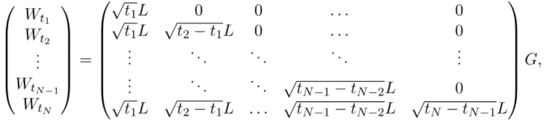
matrix involved in the Cholesky decomposition C = LL∗. To simulate W on the time-grid 0< t1 < t2 < . . . < tN, we need d×N independent standard normal variables and set
Wt1 Wt2 .. . WtN−1 WtN = √ t1L 0 0 . . . 0 √ t1L √ t2−t1L 0 . . . 0 .. . . .. . .. . .. ... .. . . .. . .. √tN−1−tN−2L 0 √ t1L √ t2−t1L . . . √ tN−1−tN−2L √ tN −tN−1L G,
where G is a normal random vector in Rd×N. The maturity time and the interest rate are respectively denoted byT >0 andr >0. The local volatility functionσ we have chosen is of the form
σ(t, x) = 0.6(1.2−e−0.1te−0.001(xert−s)2)e−0.05
√
t, (5.2)
withs > 0. We know that there exists a duality between the variables (t, x) and (T, K) in Dupire’s framework. Hence for formula (5.2) to make sense, one should choosesequal to the spot price of the underlying asset so that the bottom of the smile is located at the forward money. We refer to Figure 1 to have an overview of the smile.
Figure 1: Local volatility function
Basket option We consider options with payoffs of the form (Pd
deal with Put like options. With no surprise, we can see on Figure 2 that multilevel esti-mators always outperform their classical Monte Carlo counterpart. The comparison for very little accurate estimators may be meaningless as it is pretty difficult to reliably measure short execution times and the empirical variance of the estimator is in this case even less accurate than the estimator itself. Note that the points on the extreme right hand side are obtained for multilevel estimators withL = 2, respectively for Monte Carlo estimators with 256samples. For RMSE between 0.1 and 0.005, our MLIS estimator is 10 times faster than the standard ML estimator. When a very high accuracy is required, namely when RMSE is smaller than 0.001, the MLIS estimator remains between 3 and 4 times faster than the standard multi-level estimator, which is already a great achievement since for this multi-level of accuracy, the ML estimator may need several dozens of minutes to yield its result.
-3.5 -3.0 -2.5 -2.0 -1.5 -1.0 -2 0 2 4 log10(RMSE) lo g1 0(C PU ti me ) ML ML + IS Crude MC MC +IS
Figure 2: √M SE vs. CPU time for a basket option in the local volatility model with I = 5,
r= 0.05,T = 1,S0 = 100,K = 100,m= 4.
5.5 Multidimensional Heston model
The multidimensional Heston model can be easily written by specifying on the one hand that each asset follows a 1-D Heston model and on the other hand the correlation structure between the involved Brownian motions. The asset price process S = (S1, . . . , Sd) and the volatility
processσ = (σ1, . . . , σd) solve dSti=rSitdt+ q σi tStidBti dσti=κi(ai−σit)dt+νti q σi t(γidBti+ q 1−(γi)2dB˜i t)
where all the components ofB= (B1, . . . , Bd)andB˜ = ( ˜B1, . . . ,B˜d)are real valued Brownian motions. The vectors κ= (κ1, . . . , κd) and a= (a1, . . . , ad) denote respectively the reversion rate and the mean level of each volatility process, while the vector ν is the volatility of the volatility process. The vectorγ¯= (γ1, . . . , γd)embodies the correlations between an asset and its volatility process, withγi ∈]−1,1[ for all 1≤i≤d. The vector valued processes B and
˜
B are independent and satisfy
dhBit= ΓSdt and dhB˜it=Iddt
where we assume for our experiments that the covariance matrixΓS has the structure
ΓS= 1 ρ . . . ρ ρ 1 . .. ... .. . . .. ... ρ ρ . . . ρ 1 (5.3) withρ ∈i−1 I−1,1 h
, such that the matrixΓS is positive definite. The processes B and B˜ are
Wiener processes with covariance matrices given byΓS and Id respectively.
For the sake of simplicity, we decided not to add any extra correlation between the com-ponents of B˜, hence the choice dhB˜i =Iddt and we assume in the following that for all the γi’s are equal for 1 ≤ i ≤ d, γi = γ. The correlations between the volatilities are entirely specified by the correlations between the assets. Even though we do not aim at discussing the correlation structure of the multidimensional Heston model, we believe it is important to make precise the underlying correlation structure in the multidimensional model so that the experiments are easily reproducible.
The model can be equivalently written
dSti =rStidt+ q σi tSitdBti dσti =κi(ai−σit)dt+νti q σi tdWti
where the processesW and B are Wiener processes satisfying
dhBit= ΓSdt; dhB, Wit=γΓSdt; dhWit= (γ2ΓS+ (1−γ2)Id)dt.
The process(B, W) with values in R2dis a Wiener process with covariance matrix
Γ = ΓS γΓS γΓS γ2ΓS+ (1−γ2)Id .
factor-Basket Option We consider a basket option as in the local volatility model. Figure 3 looks very much the same as in the case of the local volatility model (see Figure 2). The MLIS estimator always outperforms all the ML estimator by a factor of 3to 4. Note that for small RMSE, the computational time can go beyond several hours, hence cutting it down by two or three times represents a real improvement.
-3.5 -3.0 -2.5 -2.0 -1.5 -1.0 -0.5 -2 -1 0 1 2 3 4 log10(RMSE) lo g1 0(C PU ti me ) ML ML + IS Crude MC MC +IS
Figure 3: √M SE vs. CPU time for a best of option in the multidimensional Heston model with I = 10, r = 0.03, T = 1, S0 = 100, K = 100, ν = 0.01, κ = 2, a = 0.04, γ = −0.2,
ρ= 0.3and m= 4.
Best of option We consider options with payoffs of the form (max1≤i≤dSTi −K)+. The payoff of this option does obviously not satisfy the assumptions of Theorem 3.2 as the payoff of the “best of” options is not Hölder withα≥1. Nonetheless, the multilevel approach beats the standard Monte Carlo technology by far (see Figure 4). Moreover, coupling importance sampling with the multilevel approach improves the accuracy. For a fixed RMSE, we can expect MLIS to be3faster that ML. This example shows the robustness of the method, which performs well whereas the theoretical assumptions are not satisfied.
6
Conclusion
We have presented a new estimator making the most of the recent works on multilevel Monte Carlo and on adaptive importance sampling. As expected, this new estimator outperforms the