Index Option Pricing Models with Stochastic Volatility and Stochastic Interest Rates

Center for

Economic Research

No. 2000-36

INDEX OPTION PRICING MODELS WITH STOCHASTIC VOLATILITY AND STOCHASTIC

INTEREST RATES

By George J. Jiang and Pieter J. van der Sluis

March 2000

Index Option Pricing Models with Stochastic Volatility and

Stochastic Interest Rates

George J. Jiang

Schulich School of Business

York University

Pieter J. van der Sluis

y

Department of Econometrics/CentER

Tilburg University

March 13, 2000

George J. Jiang, Finance Area, Schulich School of Business, York University, 4700 Keele Street, Toronto, Ontario, Canada M3J 1P3. Tel: (416) 736-2100 ext. 33302, (416) 736-5073 and Fax: (416) 736-5687. E-mail: gjiang@ssb.yorku.ca. George J. Jiang is also a SOM research fellow of the Faculty of Business and Economics at the University of Groningen in The Netherlands.

y

Pieter J. van der Sluis, Department of Econometrics/CentER, Tilburg University, P.O. Box 90153, NL-5000 LE Tilburg, The Netherlands, phone +31 13 466 2911, fax +31 13 466 3280, email: sluis@kub.nl.

Index Option Pricing Models with Stochastic Volatility and Stochastic Interest Rates

Abstract: This paper specifies a multivariate stochastic volatility (SV) model for the

S&P500 index and spot interest rate processes. We first estimate the multivariate SV model via the efficient method of moments (EMM) technique based on observations of underlying state variables, and then investigate the respective effects of stochastic interest rates, stochastic volatility, and asymmetric S&P500 index returns on option prices. We compute option prices using both reprojected underlying historical volatilities and the implied risk premium of stochastic volatility to gauge each model’s performance through direct comparison with observed market option prices on the index. Our major empirical findings are summarized as follows. First, while allowing for stochastic volatility can reduce the pricing errors and allowing for asymmetric volatility or “leverage effect” does help to explain the skewness of the volatility “smile”, allowing for stochastic interest rates has minimal impact on option prices in our case. Second, similar to Melino & Turnbull (1990), our empirical findings strongly suggest the existence of a non-zero risk premium for stochastic volatility of asset returns. Based on the implied volatility risk premium, the SV models can largely reduce the option pricing errors, suggesting the importance of incorporating the information from the options market in pricing options. Finally, both the model diagnostics and option pricing errors in our study suggest that the Gaussian SV model is not sufficient in modeling short-term kurtosis of asset returns, an SV model with fatter-tailed noise or jump component may have better explanatory power.

Keywords: Stochastic Volatility, Efficient Method of Moments (EMM), Reprojection,

Option Pricing.

1

Introduction

Numerous recent studies on option pricing have acknowledged the fact that volatility changes over time in time series of asset returns as well as in the empirical variances implied from option prices through the Black & Scholes (1973) model. Many of these studies focused on modelling the asset-return dynamics through stochastic volatility (SV) models1

. Due to analytically intractable likelihood functions and hence the lack of available efficient estimation procedures, SV models were until re-cently viewed as an unattractive class of stochastic processes compared to other time-varying volatility processes, such as ARCH/GARCH models. Moreover, to calculate option prices based on SV models we need, besides parameter estimates, a representation of the unobserved historical volatility, which is again far from being straightforward to obtain. Therefore, while the SV generalization of option pric-ing has, thanks to advances in econometric estimation techniques, recently been shown to improve over the Black-Scholes model in terms of the explanatory power for asset-return dynamics, its empiri-cal implications on option pricing itself have not yet been adequately tested due to the aforementioned lack of a representation of the unobserved volatility. Can the SV generalization of the option pric-ing model help resolve the well-known systematic empirical biases associated with the Black-Scholes model, such as the volatility “smile” (e.g. Rubinstein (1985)), asymmetry of such “smile” or “smirk” (e.g. Stein (1989))? How substantial is the gain, if any, from such generalization compared to rel-atively simpler models? The purpose of this paper is to answer the above questions by studying the empirical performance of SV models in pricing options on the S&P500 index, and investigating the re-spective effect of stochastic interest rates, stochastic volatility, and asymmetric asset returns on option prices in a multivariate SV model framework.

The structure of this paper is as follows. Section 2 outlines our model and methodology. Section 3 discusses estimation of our model. Section 4 reports our estimation results for our general model and various submodels. Section 5 compares among different models the performance in pricing options and analyses the effect of each individual factor. Section 6 concludes.

2

The Model and Methodology

2.1

The Model

We specify and implement a dynamic equilibrium model for asset returns extended in the line of Amin & Ng (1993). Our model incorporates the effect of stochastic volatility of the underlying asset returns into option valuation and at the same time allows interest rates to be stochastic. In addition, we model the short-term interest rate dynamics and asset return dynamics simultaneously and allow for asym-metry in both asset return and interest rate dynamics.

1

Let

S

t

denote the S&P500 index at time

t

2f

1

;:::;T

gand

r

t

the interest rate at time

t

, we model

the dynamics of daily S&P500 returns and daily interest-rate changes simultaneously as a multivariate Gaussian SV process. For simplicity, the conditional mean of asset returns is assumed to be constant and the de-meaned or the unexplained stock percentage return

y

s;t

is defined as

y

s;t

:= 100

(ln

S

t

,

S

)

(1)

To allow for mean reversion in the interest rate process, an autoregressive term for the conditional mean is assumed and the de-meaned or unexplained interest-rate change

y

r;t

is defined as

y

r;t

:= 100

(ln

r

t

,

r

,

r

ln

r

t

,1

)

(2)

and,

y

s;t

and

y

r;t

are modeled as SV processes

y

s;t

=

s;t

s;t

;

ln

2

s;t

+1

=

!

s

+

s

ln

2

s;t

+

s

s;t

;

j

s

j

<

1

(3)

y

r;t

=

r;t

r;t

;

ln

2

r;t

+1

=

!

r

+

r

ln

2

r;t

+

r

r;t

;

j

r

j

<

1

(4) where 2 4

s;t

r;t

3 5

IIN

(

2 4

0

0

3 5

;

2 4

1

1

1

1

3 5

)

;

j

1 j

1

(5) so thatCor

(

s;t

;

r;t

) =

1

:

Here

IIN

denotes identically and independently normally distributed.

When

1

= 0

, we have two independent asset return and interest rate processes. The asymmetry, i.e.

the correlation between

s;t

and

s;t

and between

r;t

and

r;t

;

is modelled through

2and

3as follows

s;t

=

2

s;t

+

q

1

,

2 2

u

t

;

r;t

=

3

r;t

+

q

1

,

2 3

v

t

(6) where

u

t

and

v

t

are assumed to be

IIN

(0

;

1)

withj

2

j

1

andj

3

j

1

and are uncorrelated with

s;t

and

r;t

respectively. For simplicity and ease of identification, we assume that

u

t

is uncorrelated with

v

t

. This implies

Cor

(

s;t

;

s;t

) =

2

;

Cor

(

r;t

;

r;t

) =

3 (7)

which imposes the restrictionCor

(

s;t

;

r;t

) =

1

2

3.

The SV model specified above offers a flexible distributional structure in which the correlation be-tween volatility and stock returns or interest-rate movements serves to control the level of asymmetry and the volatility variation coefficients serve to control the level of kurtosis. The above model setup is specified in discrete time and can be viewed as approximations of continuous-time SV models. The interest rate model (2) admits possible mean-reversion in the drift and allows for stochastic conditional volatility. Since the model deals with logarithmic interest rates the nominal interest rates are restricted to be positive. As a multivariate process, the above model specification allows the movements of de-meaned asset return and interest rate processes to be correlated through random noises

s;t

and

r;t

via

their correlation

1. 2

Finally, since

s;t

and

s;t

are allowed to be correlated with each other, the model can pick up the kind of asymmetric behaviour which is often observed in asset price changes and to a lesser degree in index returns and interest rate movements. In particular, a negative correlation be-tween

s;t

and

s;t

(

2

<

0

) induces the leverage effect; see Black (1976). It is noted that the above

model specification will be tested against alternative nested specifications.

Statistical properties of discrete-time SV models are discussed in Taylor (1994) and summarized in Ghysels et al. (1996) and Shephard (1996). Notably,

y

s;t

is stationary if and only if

ln

2

s;t

is stationary and

y

r;t

is stationary if and only if

ln

2

r;t

is stationary. Since

s;t

and

r;t

are assumed to be normally distributed,

ln

2

s;t

and

ln

2

r;t

are also normally distributed. The unconditional moments of

y

s;t

and

y

r;t

are given by E

[

y

s;t

] =

E

[

s;t

]exp

f

E

[ln

2

s;t

]

=

2 +

2 Var

[ln

2

s;t

]

=

8

g (8) and E

[

y

r;t

] =

E

[

r;t

]exp

f

E

[ln

2

r;t

]

=

2 +

2 Var

[ln

2

r;t

]

=

8

g (9)

which are zero for odd

. In particular, Var

[

y

s;t

] = exp

fE

[ln

2

s;t

] +

Var

[ln

2

s;t

]

=

2

g, Var

[

y

r;t

] =

exp

fE

[ln

2

r;t

] +

Var

[ln

2

r;t

]

=

2

g, and more interestingly, the kurtosis of

y

s;t

and

y

r;t

are given by

3exp

fVar

[ln

2

s;t

]

gand

3exp

fVar

[ln

2

r;t

]

gwhich are greater than

3

, so that both

y

s;t

and

y

r;t

exhibit

excess kurtosis and thus fatter tails than

s;t

and

r;t

respectively. This is true even when

s

=

r

= 0

.

2.2

Advantages of the Model and Testing Methodology

Advantages of the proposed model include: First, the model explicitly allows for stochastic interest rates. Existing work of extending the Black-Scholes model has moved away from considering either stochastic volatility or stochastic interest rates. Examples of considering both stochastic interest rates and stochastic volatility include Bailey & Stulz (1989), Amin & Ng (1993), and Scott (1997). Simu-lation results show that there can be a significant impact of stochastic interest rates on option prices; see e.g. Rabinovitch (1989). Second, the above proposed model allows the study of the simultaneous effects of stochastic interest rates and stochastic index-return volatility on the valuation of options. It is documented in the literature that when the interest rate is stochastic the Black-Scholes option-pricing formula tends to underprice the European call options (Merton (1973)), while in the case that

2

Empirical findings, in e.g. Bakshi, Cao & Chen (1997), suggest that stochastic interest rates have minimal impact on S&P 500 index option prices. However, the available empirical analysis has in general assumed that there is no correlation between asset returns and interest rates. Our findings in Section 3 that

1is insignificantly different from zero not only offers

certain justification for the above assumption but also offers further explanations to why the stochastic behaviour of interest rates has no significant impact on option prices. Moreover, the available empirical analysis has also in general assumed that the volatility of the interest rate process is constant, e.g. a diffusion process with constant volatility. However, empirical results in Andersen & Lund (1997) suggest that the volatility of short-term interest rate is stochastic. The multivariate SV model specified in this paper offers a more general framework to investigate the impact of stochastic interest rate on option prices.

the index return’s volatility is stochastic, the Black-Scholes option pricing formula tends to overprice at-the-money European call options (Hull & White (1987)). The combined effect of both factors de-pends on the relative variability of the two processes (Amin & Ng (1993)). Finally, when the asset return distribution is symmetric, i.e. there is no correlation between return and conditional volatility or

2

= 0

, the closed-form solution of the option-pricing formula is available and preference free

under quite general conditions. Let

C

0 represent the value of a European call option at

t

= 0

with

exercise price

K

and expiration date

T;

Amin & Ng (1993) derive that

C

0

=

E 0

[

S

0

(

d

1

)

,

K

exp(

,

T

,1 X

t

=0

r

t

)(

d

2

)]

(10) where

d

1

= ln(

S

0

=

(

K

exp(

, P

Tt

=0

r

t

)) +

1 2 P

Tt

=1

s;t

(

P

Tt

=1

s;t

)

1

=

2

; d

2

=

d

1 ,

T

X

t

=1

s;t

(11)

and

(

)

is the CDF of the standard normal distribution, where the expectation is taken with respect to

the risk-neutral measure and can be calculated from simulations. As Amin & Ng (1993) point out, sev-eral option-pricing formulas in the literature are special cases of the above option formula, including the Black & Scholes (1973) formula with both constant conditional volatility and interest rate, the Hull & White (1987) stochastic volatility option valuation formula with constant interest rate, the Bailey & Stulz (1989) stochastic volatility index option-pricing formula with stochastic interest rates, and the Merton (1973), Amin & Jarrow (1992), and Turnbull & Milne (1991) stochastic interest-rate option-valuation formula with constant conditional volatility. The model we study in this paper contains all above models, including the Amin & Ng (1993) model, as special cases.

The testing strategy in this paper is different in spirit from the implied methodology often used in the finance literature. As Bates (1996b) points out, the major problem of the implied estimation method is the lack of associated statistical theory, thus the implied methodology based on solely the information contained in option prices is purely objective driven. It is rather a test of stability of cer-tain relationship (the option pricing formula) between different input factors (the implied parameter values) and the output (the option prices). Instead of implying parameter values from market option prices through option pricing formulas, in this paper we directly estimate the model specified under the objective measure from the observations of underlying state variables. By doing so, the underlying model specification can be tested in the first hand for how well it represents the true data generating process (DGP), and various risk factors, such as systematic volatility risk and interest rate risk, can be identified from historical movements of underlying state variables.

We employ the EMM estimation technique of Gallant & Tauchen (1996) to estimate some candi-date multivariate SV models for daily S&P500 index returns and daily short-term interest rates. The EMM technique shares the advantage of being valid for a whole class of models with other moment-based estimation techniques, and at the same time it achieves the first-order asymptotic efficiency of

likelihood-based methods. In addition, the method provides information for the diagnostics of the un-derlying model specification. We further examine the effects of different elements considered in the model on S&P500 index option prices through direct comparison with observed market option prices. All comparisons are based on out-of-sample performance. We first compute option prices for stochas-tic volatility model based on the reprojected underlying historical volatilities and the assumption of diversifiable volatility risk, i.e. a zero volatility risk premium, and then based on the reprojected un-derlying historical volatilities and the implied stochastic volatility risk premium.3

In gauging the em-pirical performance of alternative option pricing models, we use the relative difference to measure option pricing errors.

Our methodology is also different from other research based on observations of underlying state variables. First, different from the method of moments or GMM4

used in Wiggins (1987), Scott (1987), Chesney & Scott (1989), Jorion (1995), and Melino & Turnbull (1990), the efficient method

of moments (EMM) used in this paper yields efficient estimates of SV models as we shall see below,

and the parameter estimates are not sensitive to the choice of particular moments. Second, our model allows for a richer structure for the state variable dynamics, for instance the simultaneous modeling of index returns and interest rate dynamics and asymmetry in both asset return and interest rate distri-butions.

3

Estimation and Reprojection

In this paper we employ EMM of Gallant & Tauchen (1996). This is a recent simulation-based es-timation technique for models for which standard direct maximum likelihood techniques are infea-sible or analytically intractable, but from which one can simulate sampling observations. Examples are general-equilibrium models, auction models and Stochastic Volatility (SV) models. As is apparent from its name EMM is a moment-based estimation technique. The adjective efficient is motivated by the fact that for a specific choice of the moments the EMM estimator is first-order asymptotically ef-ficient: so EMM is a GMM-type estimation technique that does as well as maximum likelihood. The common practice in the GMM literature is to select a few low-order moments on an ad hoc basis. Rec-ognizing the need for higher statistical efficiency, Gallant and Tauchen propose EMM in an article

en-3

The use of reprojected underlying volatility series in our testing is justified by at least the following two reasons. First, as the specification of underlying model varies, the volatility series is always model dependent and thus should be reprojected based on specific models. Second, in the option pricing stage, with the volatility series reprojected from underlying state variables, the risk premium of stochastic volatility is implied from option prices observed in the options market. Following this procedure, the information contained in the observed market option prices (i.e. the derivative information) is distangled from that contained in the underlying state variables (i.e. the primitive information). Compared to the case that both volatility and its risk premium are implied from option prices, the implied risk premium in our case is obviously a more sensible measure of investors’ preference toward risk.

4

titled — “Which Moments to Match?” —. The answer to this question is given in the paper: the score vector of an auxiliary probability model that fits the data well. In Gallant & Long (1997) it is shown that when this auxiliary model is chosen well, the maximum-likelihood efficiency can be obtained. In the EMM jargon the auxiliary model is also called score generator. One way to obtain efficiency for EMM is to require that the auxiliary model embeds the structural model. This embedding is hard to verify in practice. However, in Gallant & Long (1997) additional results regarding efficiency for EMM estimators are provided. Here it is shown that when the score generator has a specific data-dependent expansion, it can closely approximate the actual distribution of the data and therefore provides under very general conditions nearly fully efficient estimators. Monte Carlo studies for this specific and more general SV models in van der Sluis (1999) confirm the efficiency claim for finite samples, provided a proper leading term is chosen in the expansion. The choice of this leading term will be explained in the next subsections.

3.1

EMM Estimation

In short the EMM method is as follows5

: The sequence of densities for the structural model, namely in our case the SV model specified in Section 2.1, is denoted by

f

p

1

(

x

1 j

)

;

f

p

(

y

t

j

x

t

;

)

g 1

t

=1 g (12)

The sequence of densities for the auxiliary model is denoted by

f

f

1

(

x

1 j

)

;

f

f

(

y

t

j

x

t

;

)

g 1

t

=1 g (13)

where

x

t

is a vector of observable endogenous variables. In our case

x

t

is a vector of lagged

y

t

:

Here

is a

k

-dimensional vector of structural parameters and

an

l

-dimensional vector of auxiliary param-eters (

l

k

). Define

m

(

;

)

as

m

(

;

) =

Z Z

@

@

ln

f

(

y

j

x;

)

p

(

y

j

x;

)

dyp

1

(

x

j

)

dx

(14)

i.e. the expected score of the auxiliary model under the structural model. Since we do not have a closed form expression for (14), we determine this integral by standard Monte Carlo techniques as

m

N

(

;

) = 1

N

X

N

=1

@

@

ln

f

(

y

(

)

j

x

(

)

;

)

(15)

where

y

(

)

denote simulations from the structural model. Here

N

will typically be large. Recall that

T

denotes sample size, the EMM estimator

b

T

(

I

T

)

is defined as b

T

(

I

T

) = arg min

2

m

0

N

(

;

b

T

)(

I

T

)

,1

m

N

(

;

b

T

)

(16) 5

where I

T

is a weighting matrix and b

T

denotes a consistent estimator for the parameter of the auxiliary model to be specified below. The optimal weighting matrix here is I

0

=

lim

T

!1

V

0

[

1 p

T

P

Tt

=1 f

@@

ln

f

(

y

t

j

x

t

;

)

g

]

, where

is a (pseudo) true value. A consistent estima-tor forI

0is given by the outer product gradient. Finally, Gallant & Tauchen (1996) prove consistency

and asymptotic normality of the resulting EMM estimator

b

T

in (16), i.e. p

T

(

b

T

,

0

)

!

N

(0

;

[

M 0 0 I ,1 0 M 0

]

,1

)

where in the notation the dependence of

b

T

onI

T

will be dropped in case the optimalI

T

is used. Here M

0

=

@@

0

m

(

0

;

)

and

0denotes the true value of

:

As argued above to justify the efficiency claim6

, it is required that the auxiliary model embeds the structural model (Gallant & Tauchen (1996)) or that the structural model is located in e.g. the SNP hierarchy, which is a data-dependent expansion. The SNP density has been used in conjunction with SV models in several studies see e.g. Gallant & Tauchen (1996) and Gallant & Long (1997). For the efficiency claim to hold in our case we need Assumptions 1 to 4 from Gallant & Long (1997) to hold. Assumptions 1 and 2 can be easily verified for the SV model considered in this paper provided the parameters are such that the model is stationary and ergodic, i.e.j

s

j

<

1

andj

r

j

<

1

. Assumption 3

for the SV model is not so easy to verify at first sight and requires a formal proof that would fall outside the scope of this paper. For this assumption we refer to Andersen & Lund (1997) and Gallant, Hsieh & Tauchen (1997) where it was claimed –without explicit proof– for similar SV models that Assumption 3 holds. Assumption 4 holds because we use the SNP density as our auxiliary model. This is explicitly proved in Gallant & Long (1997).

The SNP hierarchy is built as follows. Let

y

t

be the process under investigation, let

t

=

E

t

,1

[

y

t

]

be the conditional mean of some auxiliary model, let

H

t

=

Cov

t

,1

[

y

t

,

t

]

be the conditional variance

matrix of this auxiliary model and let

z

t

=

R

,1

t

[

y

t

,

t

]

be the standardized process derived from this

auxiliary model, where

R

t

R

0

t

=

H

t

:

Here

R

t

is typically a lower or upper triangular matrix. The SNP density takes the following form

f

(

y

t

;

) =

1

j

det(

R

t

)

j

[

P

K

(

z

t

;x

t

)]

2

(

z

t

)

R

[

P

K

(

u;x

t

)]

2

(

u

)

du

(17) where

denotes the standard multinormal density,

x

t

= (

y

t

,1

;:::;y

t

,

M

)

(18)

and the polynomials are defined as

P

K

(

z;x

t

) =

K

z X

i

=0

a

i

(

x

t

)

z

i

=

K

z X

i

=0

[

K

x X

j

=0

a

ij

x

j

t

]

z

i

(19) 6

For the polynomials we use orthogonal Hermite polynomials7

. We refer to Gallant, Hsieh & Tauchen (1991) for details on the above SNP density. In the SNP terminology the parametric auxiliary model

y

t

=

N

n

(

t

;H

t

)

is labelled the leading term of the Hermite expansion. The leading term is used to relieve the Hermite expansion of some of its task. Using a proper leading term dramatically improves the small sample properties of EMM. In Andersen & Lund (1997) it is argued that in case a good leading term is used, we can set

M

= 1

in (18). We follow their advice here. Note that the vector of auxiliary parameters

consists of the parameters from the conditional mean

t

and covariance process

H

t

(the leading term parameters) and the parameters

a

ij

from the Hermite polynomials.

The problem of picking the right leading term and the right order of the polynomial

K

x

and

K

z

remains an open issue in EMM estimation. A choice that is advocated in Gallant & Tauchen (1996) is to use model specification criteria such as the Akaike Information Criterion (AIC), the Schwarz Criterion (BIC) or the Hannan-Quinn Criterion (HQC). However, the theory of model selection in the context of SNP models is not very well developed yet. In this paper the choice of the leading term and the order of the polynomials will be guided by Monte Carlo studies in van der Sluis (1999). In these Monte Carlo studies it is shown that with a good leading term for this specific and more general SV models there is no reason to employ high order Hermite polynomials, if at all, for efficiency. We will return to this issue in Section 4.1 where the leading term for our specific implementation of EMM is presented. Note that in case

K

x

= 0

, letting

K

z

>

0

induces a time-homogeneous non-Gaussian error structure. The case

K

x

>

0

induces heterogeneous innovation densities beyond that of the leading term. In applications

K

x

>

0

will often not be necessary since we will pick the leading term in such a way that it captures virtually all heterogeneity. This is also very much supported by our empirical findings.

One may deduce an omnibus test from the EMM criterion function similar to the

J

-test for overi-dentifying restrictions in the GMM literature. Under the null hypothesis that the structural model is true, we have

T

m

0

N

(

b

T

;

b

T

)(

b I

T

)

,1

m

N

(

b

T

;

b

T

)

!

d

2

l

,

k

(20)

where we recall that

k

denotes the dimension of

and

l

denotes the dimension of

. The direction of the misspecification may be indicated by the quasi-t ratios

QT

d

T

defined as d

QT

T

=

S

b ,1

T

p

Tm

N

(

b

T

;

b

T

)

(21) where b

S

T

=

f

diag[

b I

T

, c M

T

(

c M 0

T

b I ,1

T

c M

T

)

,1 c M 0

T

]

g 1

=

2 (22) and c M

T

=

@m

( b

T

;

b

T )

@

:

Note that each component of

QT

d

T

has a standard normal asymptotic distribu-tion. In particular, if a component of

QT

d

T

corresponding to a parameter in the Hermite polynomial

7 Whenzis a vector(z1;:::;zk) 0 , the expressionz i should be read asz i =z i 1 1 z i 2 2 z i k k where P k j=1 ij = iand ij0forj2f1;:::;kg:

causes rejection of the model, we know this is due to unexplained non-Gaussianity beyond that con-tained in the leading term and if a component corresponding to a specific parameter in the auxiliary leading term causes the rejection, we have an indication for the direction of misspecification of the structural model.

In principle for full efficiency one should simultaneously estimate all structural parameters, in-cluding the mean parameters

S

;

r

and

r

in (1) and (2) and all volatility parameters in (3) to (7). However, for simplicity and computational ease, we carried estimation out in the following way. First, we estimate

S

and retrieve

y

s;t

, estimate

r

and

r

and retrieve

y

r;t

, using standard regres-sion techniques in both cases. In the case that the model is covariance stationary this will yield the most efficient linear estimators for

S

and

r

and

r

:

In the literature this procedure is called

pre-whitening and is a common procedure in the literature on SV model estimation, see e.g. Sandmann

& Koopman (1998) and Harvey & Shephard (1996). Next, we simultaneously estimate parameters

= (

!

s

;!

r

;

s

;

r

;

s

;

r

;

1

;

2

;

3

)

0

of the SV model via EMM.

EMM estimation of stochastic volatility models can be rather time-consuming. Moreover many of the above stochastic volatility models have never actually been efficiently estimated. Therefore to prevent from a plethora of parameters to be estimated through EMM we use the auxiliary model, which will be a multivariate generalization of the EGARCH model of Nelson (1991), as a guidance to help to determine which of the parameters in the above SV models could be set a priori to zero for our data set. Specifically, when a parameter in this multivariate EGARCH model is estimated insignificantly different from zero and there exists a clear correspondence to a parameter in the SV model we set this SV parameter equal to zero a priori. The multivariate EGARCH (MEGARCH) model we employ as a leading term in the SNP density is the following.

2 4

y

s;t

y

r;t

3 5

=

2 4

h

s;t

0

0

h

r;t

3 5 2 4

z

s;t

z

r;t

3 5 (23)

ln

h

2

s;t

=

0

s

+

ss

ln

h

2

s;t

,1

+

sr

ln

h

2

r;t

,1

+

(1 +

s

L

)[

1

;s

z

s;t

,1

+

2

;s

(

j

z

s;t

,1 j, q

2

=

)]

(24)

ln

h

2

r;t

=

0

r

+

rr

ln

h

2

r;t

,1

+

rs

ln

h

2

s;t

,1

+

(1 +

r

L

)[

1

;r

z

r;t

,1

+

2

;r

(

j

z

r;t

,1 j, q

2

=

)]

(25) 2 4

z

s;t

z

r;t

3 5

=

IIN

(0

;

2 4

1

1

3 5

)

(26)

Here

L

denotes the lag operator. As in (17) the MEGARCH model is expanded with the Hermite polynomials which allow for nonnormality. The parameter

in the MEGARCH model corresponds to

1in the SV model. The

’s, possibly in combination with some of the parameters of the polynomial,

correspond to

2and

3

:

This latter correspondence is further investigated in a Monte Carlo study in

exists a clear correspondence from the EGARCH model to the SV model, e.g.

ss

corresponds to

s

and

0

s

corresponds to

!

s

:

We report estimation results in Section 4.1 below.

3.2

Volatility Reprojection

One of the criticisms on EMM and on moment-based estimation methods in general has been that the method does not provide a representation of the unobservables in terms of their past, which can be obtained from the prediction-error-decomposition in likelihood-based techniques. In the context of SV models this means that we lack a representation of the unobserved volatilities f

s;t

g

Tt

=1 and f

r;t

g

Tt

=1 as we need these series in our option pricing formula (10). The reprojection technique of

Gallant & Tauchen (1998) overcomes this problem.

Reprojection is projecting a long simulated series from the estimated structural model

p

on the auxiliary model

f

. In short reprojection is as follows. We define the estimator

;

e

different from

;

b as follows e

:= arg max

E b

T

f

(

y

t

j

x

t

;

)

(27)

where as in Section 3

x

t

contains observable endogenous variables. In our case

x

t

is a vector of lagged

y

t

:

NoteE b

T

f

(

y

t

j

x

t

;

)

is calculated using one set of simulations f

y

(

b

T

)

g

N

=1 from the structural

model in the same vein as (15). Results in Gallant & Long (1997) show that

lim

K

!1

f

(

y

t

j

x

t

;

e

K

) =

p

(

y

t

j

x

t

;

b

)

(28)

where

K

is the overall order of the leading term and the Hermite polynomials should grow with the sample size

T;

either adaptively as a random variable or deterministically, similarly to the estimation stage of EMM. Due to (28) the (conditional) moments under the structural model in

b

T

can be calcu-lated using the auxiliary model in

e.

A more common notion of filtration is to use the information on the observables

y

t

up to and in-cluding time

t

, instead of

t

,

1

, since we want a representation for unobservables in terms of the past

and present observables. Indeed for option pricing it is more natural to include the present observables

y

t

, as we have current stock price and interest rate in the information set. Following Gallant & Tauchen (1998) we can repeat the above derivation with

y

t

replaced by

ln

2

t

, and

y

t

included in the informa-tion set at time

t

. In this case we need a different auxiliary model

f

(ln

2

t

j

y

t

;y

t

,1

;:::;y

t

,

L

;

)

from

the one used in the estimation stage,

f

(

y

t

j

x

t

;

)

, where we note that

x

t

only contained lagged values

of

y

t

:

More precisely, we need to specify an auxiliary model for

ln

2

t

using information up till time

t;

instead of

t

,

1

;

as in the auxiliary EGARCH model. Since with the sample size in this application

projection on pure Hermite polynomials may not be a good idea due to small sample distortions and issues of non-convergence, we use the following intuition to build a useful leading term. Omitting the

subscripts

s

and

r;

we can write (3) or (4) as

ln

y

2

t

= ln

2

t

+ ln

2

t

(29)

As argued in Harvey, Ruiz & Shephard (1994) the process for

ln

y

2

t

is a non-Gaussian ARMA

(1

;

1)

process. We therefore consider the following auxiliary model for

ln

2

t

ln

2

t

=

0

+

L

r X

i

=1

i

ln

y

2

t

,

i

,1

+

error

(30)

where the lag-length

L

r

will be determined by AIC. For model (30), expressions for

ln

b 2 0

=

E

(ln

2 0 j

y

0

;:::;y

,

L

r

+1

)

follow straightforwardly. Formula (30) can be viewed as the update equation

for

ln

2

t

of the Gaussian Kalman filter of Harvey et al. (1994). In this update equation we have ex-tra restrictions on the coefficients

0 to

L

r

:

Since we are able to determine these coefficients with

arbitrary precision by Monte Carlo simulation there is no need to work out these restrictions. Note that the original Harvey et al. (1994) Kalman filter approach is sub-optimal for the SV models that are considered here: an exact filter would require a non-Gaussian Kalman filter approach. In this case the update equation for

ln

2

t

is not a linear function of

ln

y

2

t

and lagged

ln

y

2

t

:

It will basically downweight outliers so the weights are data-dependent. The fact that the restrictions on the coefficients on

0 till

L

r are not those imposed by the sub-optimal Gaussian Kalman Filter but estimated using the true SV

model will have the effect that the linear approximation used here is based on the right model instead of the wrong model as in the Harvey et al. (1994) case. Though, an Hermite expansion of the model (30) as in the estimation stage should asymptotically overcome the suboptimality of the proposed fil-ter, we will in this paper not use the Hermite expansion. We do this for the following reasons: (i) Since

e

in (27) must be determined by ML in case an SNP density is specified with (30) as a leading term where

L

r

is large, the resulting problem is a very high dimensional optimization problem resulting in all sorts of problems (ii) In some simulation experiments we investigated the differences between the reprojected volatilities

ln

b

2

t

using no Hermite expansion and the true volatilities

ln

2

t

. There was very strong evidence that these errors are normally distributed, without any systematic error components. Further research should be conducted to address these issues. Also note that our reprojection approach is similar to the approach taken in Chernov & Ghysels (1999) though they reproject on lagged Black Scholes volatilities implied from the option prices, rather than on lagged

ln

y

2

t

:

For the asymmetric model, we should, as in the EGARCH model, include components able to capture the asymmetry. Therefore we propose to consider

ln

2

t

=

0

+

0

+

L

r X

i

=1

i

ln

y

2

t

,

i

,1

+

L

s X

j

=1

j

y

t

,

j

t

,

j

+

error

(31)

Here there is no known relation between the update formula for

ln

2

t

from the Kalman Filter and the

y

t,j

t,j

terms. However since the coefficients of

j

are highly significant in the applications and in sim-ulation studies, this model is believed to be a good leading term for reprojection. This is backed up by

the fact that in simulation experiments (not reported) the same properties of the errors

ln

b 2

t

,

ln

2

t

were observed as in the symmetric model above.

For reprojecting volatility series in the multivariate case we can use ideas described in van der Sluis (1999): first transform the correlated

y

r;t

and

y

s;t

to uncorrelated series (which can be achieved by means of a Choleski-decompostion) and then apply the univariate reprojection method described above to each of the uncorrelated series.

4

Empirical Results

4.1

Description of the Data

The time-series observations of the S&P 500 index consist of daily observations over the period from 1980 to 1995. The data observed over 1980 through 1994 are used to estimate the model for the pur-pose of pricing options on the index. We set aside the last year of data (1995) in order to perform the out-of-sample tests. To adjust for dividends of the S&P 500 index, a continuously compound rate of

2%

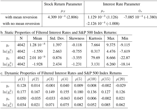
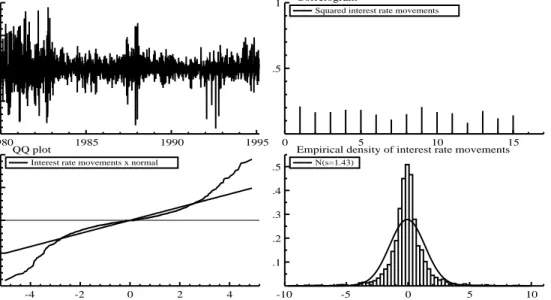
was used for simplicity, which is consistent with the practice in Boyle, Broadie & Glasserman (1997). To estimate the spot interest rate model, the US 3-month T-bill rates are used as proxy of the “instantaneous” rates. The data are also daily, covering the same sampling period 1980 to 1995. As justified in Jiang (1998), the use of a 3-month rate is a necessary compromise between literately taking an “instantaneous” rate, say overnight rates, and avoiding some of the associated spurious microstruc-ture effects.

The summary statistics of both static and dynamic properties of daily S&P 500 index and 3-month T-bill rates over 1980 to 1995 are reported in Table 1, a time-series plot and salient features of both data sets can be found in Figures 1 and 2. Estimates of conditional mean parameters are also reported in Table 1. For logarithmic interest rates, there is an insignificant linear mean-reversion, which is consis-tent with many findings in the literature. In our estimation, the conditional mean is assumed constant. From Table 1, we can see that both the de-meaned returns of S&P 500 index and interest rates are skewed to the left and have positive excess kurtosis (

>>

3

) suggesting skewed and fat-tailed distribu-tions. Obviously, the 1987 crash contributes to both the negative skewness and positive excess kurto-sis. However, the logarithmic squared filtered series, as proxy of the logarithmic conditional volatility, only have small excess kurtosis and appear to justify the Gaussian stochastic volatility process. As far as dynamic properties, the filtered interest rates and index returns as well as logarithmic squared fil-tered series are all temporally correlated. For the logarithmic squared filfil-tered series, the first order autocorrelations are in general low, but higher order autocorrelations are of similar magnitudes as the first order autocorrelations. This would suggest that all series are roughly ARMA

(1

;

1)

or equivalently AR

(1)

with measurement error, which is consistent with the first order autoregressive SV model spec-ification.

Since the score generator should give a good description of the data, we further look at the data through specification of the score generator or auxiliary model. As explained in the previous section we use the score generator as a guide for the structural model, as there is a clear relationship between the parameters of the auxiliary model and the structural model. If some auxiliary parameters in the score generator are not significantly different form zero, we set the corresponding structural parameters in the SV model a priori equal to zero. Various model selection criteria and

t

-statistics of individual parameters in class of auxiliary models that was proposed in Section 3 indicate that (i) On the basis of the model selection criteria and the

t

–values of the parameter

the multivariate EGARCH(1,1) model was found to be marginally useful. We therefore include

1in our analysis; (ii) The cross terms

rs

and

sr

were significantly different from zero albeit small, again on the basis of the BIC inclusion of these parameters was not justified. Therefore our exclusion of cross terms between

ln

2

s;t

and

ln

2

r;t

in (3) and (4) is justified; (iii) Regarding the choice of a suitable order for the Hermite polynomial in the SNP expansion, we find

K

x

= 0

for all models. As argued in Section 3 this indicates that we have chosen a proper leading term in the expansion, because

K

x

>

0

would indicate that not all time-dependent non-Gaussianity is captured by the leading term. Regarding

K

z

we find that according to the most conservative model selection criterion, i.e. the BIC we should take up a considerable high order of the Hermite polynomial corresponding to the time-homogeneous non-Gaussianity. This is undesirable because Monte Carlo results in van der Sluis (1999) indicate that for sample sizes encountered here the order of the Hermite polynomial should be low, say 4 or 5 and that under the null of a Gaussian SV model, setting the order to zero will yield virtually efficient estimates. It was also found in van der Sluis (1999) that for estimating a symmetric SV model

(

2

= 0)

the use of a symmetric score generator

(

2

= 0)

slightly improves over an asymmetric score generator. However it is important to consider

the auxiliary model with

K

z

>

0

. Consider the conditional density implied by the ML estimates using optimal values for

K

z

for both data sets in Figures 3 and 4. Clearly, there is evidence in the data that a Gaussian EGARCH model does not fully capture the time-homogeneous excess kurtosis. It also appears that for

K

z

>

10

the SNP density puts probability mass at outliers. For descriptive purposes such high orders in the auxiliary model can be desirable, however, since under the null of Gaussian SV we cannot get such outliers, there is no need to use high-order polynomials in the score generator. Therefore we decided for these sample sizes to set the Hermite polynomial equal to zero. To check the validity of this argument we performed EMM estimation using a moderate size of

K

z

= 6

to see whether the results would differ from the ones with

K

z

= 0

, and it turns out that the parameter estimates differ only slightly. As argued above, inspection of the individual components

QT

d

T

of the

J

-test provide information of the source of misspecification of the model. So with

K

z

= 0

the

J

-test will have no power against non-Gaussianity in the data beyond the non-Gaussianity captured by the MEGARCH model. Therefore in the next we will also consider the

J

-test for

K

z

>

0

:

4.2

Structural Models and Estimation Results

The general model: the model specified in Section 2.1 assumes stochastic volatility for both the asset returns and interest rate dynamics. This model nests the Amin & Ng (1993) model as a special case when

2

= 0

. Following are three alternative model specifications:

Submodel 1: No stochastic interest rates, i.e. interest rate is constant,

r

t

=

r

, as in the Hull &

White (1987), Johnson & Shanno (1987) and Wiggins (1987) models;

Submodel 2: Constant asset return volatility but stochastic interest rate,

s;t

=

, as in the

Merton (1973), Turnbull & Milne (1991) and Amin & Jarrow (1992) models;

Submodel 3: Constant asset return volatility and constant interest rate,

s;t

=

;r

t

=

r

, as in

the Black-Scholes model.

The results reported here are all for the MEGARCH(1,1)-H(0,0) model, where, as argued above, for estimating symmetric SV models we set

2

= 0

;

and for univariate models we set

= 0

:

As argued

in Section 4.1 the models have also been estimated setting

K

z

= 6

but no substantial differences were found in the estimation results.

The general multivariate SV (MSV) model: The estimates for the mean terms are given in Table

1 and the estimates of the multivariate SV model for both symmetric stochastic volatility and asymmetric volatility are given in Table 2. It is noted that similar to other financial time series, the persistence parameter is close to, but significantly different from, unity. The asymmetry is moderate for both series and significantly different from zero. The leverage effect is somewhat higher for the S&P500 returns than for the interest rate changes. In the reprojection stage we set the lag lenght

L

s

= 30

for both the interest rate and the S&P500 series. For reprojection with the asymmetric SV model, we set

L

s

= 30

and

L

r

= 30

for both series. These settings are based on previous experimentation. It was found that for the parameter values and sample size encountered here, AIC advocates about these lag lengths. We found it too time-consuming to determine the optimal AIC for each and every reprojection and advocate as a rule of thumb to use

L

r

=

L

s

= 30

. The filtered series for the asset returns using the symmetric and asymmetric models are displayed in Figure 5. Filtered series for the interest rates are displayed in Figure 6.

Submodels 1, 2 & 3: The estimation results of submodels 1 and 2 are also reported in Table 2.

The estimation of univariate SV models is straightforward as it is equivalent to impose

1

=

0

in the multivariate SV model. Thus submodel 1 takes the SV part of the asset returns, and submodel 2 takes the SV part of the interest rates. The estimate of the constant volatility for the non-stochastic volatility model of S&P 500 index returns in submodel 2 and submodel 3 is obtained from its sample variance.

Table 3 reports the results of the Hansen

J

-test using EMM. As we see all the models have been accepted at a 5% level. Though a

P

-value is a monotone function of the actual evidence against

H

0

;

it is very dangerous to choose the best model of these specifications on the basis of the

P

-values; see Berger & Delampady (1987). An LR test of the asymmetric SV model versus the symmetric SV model cannot be deduced from the difference in criterion values, since the criterion values are based on dif-ferent score generators. The

t

-values corresponding to the asymmetry parameter are asymptotically equivalent to a LR test using common score generators and indicate that the null hypothesis of sym-metry is rejected in favour of the alternative asymmetric model.

For the

J

-test with one degree of freedom it is not useful to consider the individual components of the test statistic as in (21)8

. In case we set

K

z

= 6

a

J

-test from the auxiliary model leads to rejection of all Gaussian SV models. By inspection of the individual components of this

J

-test (not reported) we find that in this case the rejection can completely be attributed to the Hermite polynomial. This essentially means that the Gaussian SV model cannot account for the time-homogeneous error structure beyond the EGARCH structure that is imposed by the Hermite polynomials. the values of the individual components of the

J

-test corresponding to the parameters of the Hermite polynomial cause rejection of the SV model by the

J

-test. Further research should therefore include this fact by using a structural model with fatter-tailed noise or jump component. Since such a non-Gaussian SV model will make option pricing much more complicated, we leave this for future research. The conclusion is that a Gaussian SV model may not be adequate and one should consider a fatter-tailed SV model or a

jump process. This can also be seen by comparing the sample properties of the data with the sample

properties of the SV model in the optimum.

5

Empirical Performance of Alternative Option Pricing Models

The effects of SV on option prices have been examined by simulation studies9

as well as empirical studies10

. In this paper we will investigate the implications of model specification on option prices through direct comparison with observed market option prices. As Bates (1996b) points out, funda-mental to testing option pricing models against time series data is the issue of identifying the rela-tionship between the true process followed by the underlying state variables in the objective measure and the “risk-neutral” processes implied through option prices in an artificial measure. Representative agent equilibrium models such as Rubinstein (1976), Brennan (1979), Bates (1988, 1991), and Amin & Ng (1993) among others indicate that European options that pay off only at maturity are priced as if investors priced options at their expected discounted payoffs under a model that incorporates the

8

In this case the individualt-values are all about the same. This is a consequence of the fact that the individualt-values

are asymptotically equal with probability one in case of only one degree of freedom in the test.

9

Hull & White (1987), Johnson & Shanno (1987), Bailey & Stulz (1989), Stein & Stein (1991) and Heston (1993)

10

appropriate compensation for systematic asset, volatility, interest rate, or jump risks. Similarly, the no-arbitrage models show that option prices are discounted future payoffs at the riskfree rate of inter-est under an equivalent martingale measure or the ”risk-neutral” measure, see Cox & Ross (1976) and Harrison & Kreps (1979). Thus, the corresponding “risk-neutral” specification of the general model specified in Section 2 involves compensation for various risks. More specifically, in the ”risk-neutral” specification the expected index return would be equal to the riskfree rate of interest, the drift of the interest rate process would be adjusted to incorporate the risk premium of stochastic interest rate, and the drift terms of the stochastic volatility processes for both interest rate and index return would be adjusted to incorporate the risk premiums of stochastic volatility, as we shall see later in Section 5.3. Standard approaches for pricing systematic volatility risk, interest rate risk, and jump risk have typ-ically involved either assuming the risk is nonsystematic and therefore has zero premium, or by im-posing a tractable functional form on the risk premium (e.g. the factor risk premiums are proportional to the respective factors) with extra (free) parameters to be estimated from observed options prices or bond prices (for interest rate risk).

Under the “risk-neutral” distribution of the general framework, a European call option on a non-dividend paying asset that pays off

max(

S

T

,

X;

0)

at maturity

T

for exercise price

X

is priced as

C

0

(

S

0

;r

0

;

r

0

;

S

0

;

T;X

) =

E 0

[

e

, R T 0

r

t

dt

max(

S

T

,

X;

0)

j

S

0

;r

0

;

r

0

;

S

0

]

(32) whereE

0is the expectation with respect to the “risk-neutral” specification for the state variables

con-ditional on all information at

t

= 0

. In particular, when

2

= 0

in the general model setup, i.e.

As-sumption 2 of Amin & Ng (1993) is satisfied as assumed in Hull & White (1987), the option pricing formula can be derived as in (10). Furthermore, if asset volatility is also constant, we obtain the Black-Scholes formula. Our analysis for the implications of model specification on option prices is outlined as follows:

Two different tests are conducted for alternative models. First we assume, as in Hull & White (1987) among others, that stochastic volatility risk is diversifiable and therefore has zero risk premium. Based on the reprojected underlying stochastic volatility for SV models and estimated volatility pa-rameter for constant volatility models, we calculate option prices with given maturities and moneyness. The model-generated option prices are compared to the observed market option prices in terms of rel-ative percentage differences. Second, we assume a non-zero risk premium for stochastic volatility of asset returns. As pointed out in Section 2.2, the reprojected volatility is still used, while the risk pre-mium of SV is estimated from observed option prices in the previous day. The estimates are used in the following day’s volatility process to calculate option prices, which are also compared to the observed market option prices. Throughout the comparison, all the models only rely on information available at a given time, thus the comparison is based on the out-of-sample performance. In particular, in the first comparison, all models rely only on information contained in the underlying state variables, while in

the second comparison, the models use information contained in both the underlying state variables and the observed (previous day’s) market option prices. Our study is clearly different from those which use option prices to imply all parameter values of the “risk-neutral” model, e.g. Bakshi et al. (1997). In their analysis, all the parameters and underlying volatility are estimated through fitting the option pricing model into observed option prices. Then these implied parameters and underlying volatility are used to predict the same set of option prices. In our comparison, the risk factors are identified from underlying asset return process and the preference parameters for option traders are inferred from ob-served market option prices.

5.1

Description of the Option Data

The options data set of the S&P 500 index is obtained from the CBOE for the sample period January 3, 1995 to December 29, 1995, which extends one year from the estimation sample period. Since we do not rely solely on option prices to obtain the parameter estimates through fitting the option pricing formula, such a sample size is adequate for our comparison purpose. S&P 500 Index Options (SPX) are European-type and among the most actively traded financial derivatives in the world. S&P 500 index options and options on S&P 500 futures have been the focus of many existing investigations in-cluding, among others, A¨ıt-Sahalia & Lo (1998), Bakshi et al. (1997), Bates (1996a), Dumas, Fleming & Whaley (1998), Madan, Carr & Chang (1998), Nandi (1998), and Rubinstein (1994).

The original data set contains both call options and put options. However, all the in-the-money options for both puts and calls are very infrequently traded relative to at-the-money and out-of-the-money options, in-the-out-of-the-money option prices are thus notoriously unreliable. Another issue is that the index typically pays a dividend and the future rate of dividend payment is difficult, if not impossible, to determine. As A¨ıt-Sahalia & Lo (1998) point out, even though Standard and Poor’s does provide daily dividend payments on the S&P 500, by nature these data are backward-looking, and there is no reason to assume that the actual dividends recorded ex-post correctly reflect the expected future dividends at the time the option is priced. To circumvent these problems, we use the ideas in A¨ıt-Sahalia & Lo (1998). First, we derive the implied futures

F

t;T

,

t

of the index based on the most at-the-money (i.e.

smallestj

Ke

,

r

t;T,t (

T

,

t

)

,

S

t

j) put and call option prices, as they both are actively traded options,

using the put-call parity relationship,

C

(

S

t

;t

;

K;T;r

t;

;d

t;

) +

Ke

,

r

t;

=

P

(

S

t

;t

;

K;T;r

t;

;d

t;

) +

F

t;

e

,

r

t;

(33) which must hold if arbitrage opportunities are to be avoided, regardless what option pricing model being used, where

P

(

)

is the put option price at time

t

with strike price

K

and maturity date

T

. With

the implied futures at each date

t

and options’ maturity date

T

, the dividend yield can be backed out from the following spot-futures parity,

F

t;T

,

t

=

S

t

e

(

r

t;T,t ,

d

t;T,t )(

T

,

t

) (34)

Our results show that the backed out dividend rates over the sample period are in general quite stable cross time and maturity, with its average approximately 1.8% annually. Secondly, given the implied future prices

F

t;T

,

t

, we replace the prices of all illiquid call options, i.e. the deep in-the-money

op-tions, with the prices of liquid put options at the relevant strike prices via the put-call parity. The put options are by construction out-of-the-money options and thus liquid. After this procedure, all the in-formation contained in liquid put prices has been extracted and resides in corresponding call prices. Therefore, put prices may now be discarded without any loss of reliable information.

The data set consists of intra-daily bid-ask quotes for the index options with various strike prices and expiration dates. To ease computational burden, for each business day in the sample only the last reported bid-ask quote during the trading session (i.e. prior to 3:02 PM Central Standard Time) of each option contract is used in the empirical test. The index is simultaneously observed as the option’s bid-ask quote. Therefore they are not transaction data, which avoids the issue of non-synchronous prices. A few filters are further applied to the data set. First of all, the data only include options with at least 5 days to expiration to reduce biases induced by liquidity-related issues; Secondly, option quotes which do not satisfy arbitrage restrictions are excluded. We noticed that these options are mostly those very illiquid ITM call/put options, which are all replaced by the corresponding OTM put/call option prices through the put-call parity; Thirdly, options with prices below $3/8 are also excluded as for these options the market microstructure issues, such as price discretization, demand and supply imbalance, can have strong impact on the bid and ask. Moreover, in our implied parameter estimation procedure these options carry only a minimal weight in the minimization problem.

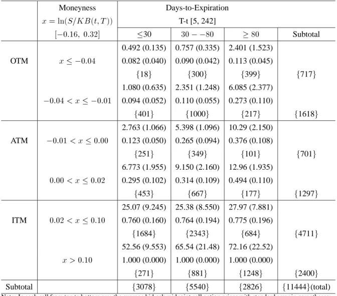
We divide the option data into several categories according to either moneyness or time to expira-tion. In this paper, we use a slightly different definition of moneyness for options from the conventional one11

. Following Ghysels et al. (1996), we define

x

t

= ln(

S

t

=Ke

, R T t

r

d

)

(35) Technically if

x

t

= 0

, the current stock price

S

t

coincides with the present value of the strike price

K

, the option is called at-the-money; if

x

t

>

0

(respectively

x

t

<

0

), the option is called in-the-money (respectively out-of-the-money). In our partition, a call option is said to be at-the-money (ATM) if

,

0

:

01

< x

0

:

02

; out-of-the-money (OTM) if

x

,

0

:

01

; and in-the-money (ITM) if

x >

0

:

02

.

A finer partition resulted in six moneyness categories as in Table 4. According to the time to expi-ration, an option contract can be classified as: i) short-term (

T

,

t

30

days); ii) medium-term

(

30

< T

,

t <

80

days); and iii) long-term (

T

,

t

80

days). The partition according to moneyness

and maturity results in 18 categories as in Table 4. For each category, the average bid-ask midpoint

11

In practice, it is more common to call an option as at-the-money/in-the-money/out-of-the-money whenSt=K =St> K =S

t

<Krespectively. For American type options with possibility of early exercise, it is more convenient to compareS t

withK, while for European type options and from an economic point of view, it is more appealing to compareStwith the

price and its standard error, the average effective bid-ask spread (i.e. the ask price minus the bid-ask midpoint) and its standard deviation, as well as the number of observations in the category are re-ported. Note that among 11,444 total observations, about 20.40% are OTM options, 17.46% are ATM options, 62.14% are ITM options; 26.90% are short-term options, 48.41% are medium-term options, and 24.69% are long-term options. The average price ranges from $0.492 for short-term deep out-of-the-money options to $72.16 for long-term deep in-the-money options, and the average effective bid-ask spread ranges from $0.082 for short-term deep out-of-the-money options to $1.000 for long-term deep in-the-money options.

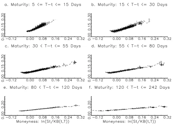
Figure 7 plots the implied Black-Scholes volatility against moneyness for options with different terms of maturity. The implied Black-Scholes volatilities are backed out from each option quote using the corresponding stock price, time to expiration, and the current yield of US treasury instruments with maturity closest to the maturity of the option. Namely, we use the 3-month T-bill rates for options with maturity less than 4 months, and 6-month T-bill rates for options with maturity longer than 4 months. All discount rates are converted to annualized compound rates. It is noted that the Black-Scholes im-plied volatility exhibits obvious shape of “smirk” as the call option goes from deep OTM to ATM and then to deep ITM, with the deepest ITM call option implied volatilities taking the highest values. The volatility “smirk” is more pronounced and more sensitive to the term to expiration for short-term op-tions than for the medium-term and long-term opop-tions. Furthermore, the volatility “smirk” is skewed to the left, as observed for most asset and index option prices. These observations indicate that the short-term options are the mostly severely mispriced ones by the Black-Scholes model and present perhaps the greatest challenge to any alternative option pricing model. These findings are consistent with those in the aforementioned studies on S&P 500 index options and studies on other securities in the literature; see e.g. Rubinstein (1985), Clewlow & Xu (1993), Taylor & Xu (1994).

5.2

Comparison based on Diversifiable Stochastic Volatility Risk

In this section, we assume that the risk premiums in both interest rate and asset return processes as well as the conditional volatility processes are all zero. That is, the risk-neutral process is assumed to be the same as the objective underlying process. The SV option prices are calculated based on Monte Carlo simulation using (32) for asymmetric models and both (10) and (32) for symmetric models, the reported results are all based on simulations. In both (10) and (32), the reprojected current underlying volatility (at the time the options are priced) is used for the SV models and the estimated historical volatility is used for the constant volatility models.12

The only approximation error involved is the

12

As the referee correctly points out, the reprojection technique can also be used for constant volatility models based on the historical observations of asset returns. However, to be consistent with the model specification of constant volatility, we use the efficient estimator of the constant volatility parameter in our application. Furthermore, in order to reproject the un-derlying stochastic volatility, ideally the model should be re-estimated each day. Due to the intensive computation involved

Monte Carlo error which can be reduced to any desirable level by increasing the number of simulations. The estimation error involved in our study is also minimal as we rely on large number of observations over long sampling period to estimate model parameters. In our simulation, 100,000 sampling paths are simulated to reduce the Monte Carlo error and to reflect accurately the fat-tail behaviour of the asset return distributions, and the antithetic variable technique is used to reduce the variation of option prices; see Boyle et al. (1997). The results show that option prices generated using different methods are almost the same, with the largest differences less than a penny for even long term deep ITM options. The accuracy is further reflected in the small standard derivations of the simulated option prices.

Option pricing biases are compared to the observed market prices based on the mean relative per-centage option pricing error (MRE) and the mean absolute relative option pricing error (MARE), given by

MRE

= 1

n

X

n

i

=1

C

i

,

C

~

i

C

i

(36)

MARE

= 1

n

X

n

i

=1 j

C

i

,

C

~

i

j

C

i

(37)

where

n

is the number of options used in the comparison,

C

~

i

and

C

i

represents respectively the ob-served market option price and the theoretical model option price. The MRE statistic measures the average relative biases of the model option prices, while the MARE statistic measures the dispersion of relative biases of the model prices. The difference between MARE and MRE suggests the direc-tion of the bias of the model prices, namely when MARE and MRE are of the same absolute values, it suggests that the model systematically misprices the options to the same direction as the sign of MRE, while when MARE is much larger than MRE in absolute magnitude, it suggests that the model is in-accurate in pricing options but the mispricing is less systematic. Since the percentage errors are very sensitive to the magnitude of option prices which are determined by both moneyness and length of ma-turity, we also calculate MRE and MARE for each of the 18 moneyness-maturity categories in Table 4.

Table 5 reports the relative pricing errors (%) for alternative models in terms of option prices. In each cell, from top to bottom are the MRE (mean relative error) and MARE (mean absolute relative er-ror) statistics for: 1. the asymmetric general SV model (aMSV) with

2

6

= 0

;

3

6

= 0

; 2. the symmetric general SV model (sMSV) with

2

=

3

= 0

; 3. the asymmetric submodel 1 (SVCI) with

2

6

= 0

and constant interest rates; 4. the asymmetric submodel 2 (CVSI) with

3

6

= 0

and constant asset return volatility; and 5. submodel 3 with constant asset return volatility and constant interest rates,

in estimating the SV model using EMM, this is infeasible. Thus the reprojection of underlying volatility is based on the model estimated using the asset returns over the sample period from 1980 to 1994. Re-estimating the model based on the extended sample period from 1980 to 1995 (i.e. including the sample period of options data), we obtained virtually the same parameter estimates, suggesting there is no significant structural break for the asset return proc