The University of Bradford Institutional
Repository
http://bradscholars.brad.ac.uk
This work is made available online in accordance with publisher policies. Please refer to the
repository record for this item and our Policy Document available from the repository home
page for further information.
To see the final version of this work please visit the publisher’s website. Access to the
published online version may require a subscription.
Link to publisher’s version:
http://dx.doi.org/10.3847/0004-637X/829/2/89
Citation:
Barnes G, Leka KD and Schrijver CJ et al. (2016) A comparison of flare forecasting
methods, I: results from the “All-clear” workshop. The Astrophysical Journal. 829(2).
Copyright statement:
© 2016 American Astronomical Association. Reproduced in accordance
with the publisher's self-archiving policy.
A COMPARISON OF FLARE FORECASTING METHODS, I: RESULTS FROM THE “ALL-CLEAR” WORKSHOP
G. Barnes and K.D. Leka
NWRA, 3380 Mitchell Ln., Boulder, CO 80301, USA
C.J. Schrijver
Lockheed Martin Solar and Astrophysics Laboratory, 3251 Hanover St., Palo Alto, CA 94304, USA
T. Colak, R. Qahwaji, O.W. Ashamari
School of Computing Informatics and Media, University of Bradford, Bradford, UK
Y. Yuan
Space Weather Research Laboratory, New Jersey Institute of Technology, Newark, NJ 07102, USA
J. Zhang
Department of Physics and Astronomy, George Mason University, 4400 University Dr., Fairfax, VA 22030, USA
R.T.J. McAteer
Department of Astronomy, New Mexico State University, P.O. Box 30001, MSC 4500, Las Cruces, NM 88003-8001, USA
D.S. Bloomfield1, P.A. Higgins, P.T. Gallagher
Astrophysics Research Group, School of Physics, Trinity College Dublin, College Green, Dublin 2, Ireland
D.A. Falconer
Heliophysics and Planetary Science Office, ZP13, Marshall Space Flight Center, Huntsville, AL 35812, USA ; Physics Department, University of Alabama in Huntsville, AL 35899, USA ; Center for Space Plasma and Aeronomic Research, University of Alabama in
Huntsville, AL 35899, USA
M.K. Georgoulis
Research Center for Astronomy and Applied Mathematics (RCAAM), Academy of Athens, 4 Soranou Efesiou Street, Athens 11527, Greece
M.S. Wheatland
Sydney Institute for Astronomy, School of Physics, The University of Sydney, NSW 2006, Australia
C. Balch
T. Dunn and E.L. Wagner
NWRA, 3380 Mitchell Ln., Boulder, CO 80301, USA
1
Department of Physics and Electrical Engineering, Northumbria University, Newcastle Upon Tyne, NE1 8ST, UK
ABSTRACT
Solar flares produce radiation which can have an almost immediate effect on the near-Earth environ-ment, making it crucial to forecast flares in order to mitigate their negative effects. The number of published approaches to flare forecasting using photospheric magnetic field observations has prolifer-ated, with varying claims about how well each works. Because of the different analysis techniques and data sets used, it is essentially impossible to compare the results from the literature. This problem is exacerbated by the low event rates of large solar flares. The challenges of forecasting rare events have long been recognized in the meteorology community, but have yet to be fully acknowledged by the space weather community. During the interagency workshop on “all clear” forecasts held in Boulder, CO in 2009, the performance of a number of existing algorithms was compared on common data sets, specifically line-of-sight magnetic field and continuum intensity images from MDI, with consistent definitions of what constitutes an event. We demonstrate the importance of making such systematic comparisons, and of using standard verification statistics to determine what constitutes a good prediction scheme. When a comparison was made in this fashion, no one method clearly outperformed all others, which may in part be due to the strong correlations among the parameters used by different methods to characterize an active region. For M-class flares and above, the set of methods tends towards a weakly positive skill score (as measured with several distinct metrics), with no participating method proving substantially better than climatological forecasts.
Keywords: methods: statistical – Sun: flares – Sun: magnetic fields
1. INTRODUCTION
Solar flares produce X-rays which can have an almost immediate effect on the near-Earth environment, especially the terrestrial ionosphere. With only eight minutes delay between the event occurring and its effects at Earth, it is crucial to be able to forecast solar flare events in order to mitigate negative socio-economic effects. As such, it is desirable to be able to predict when a solar flare event will occur and how large it will be prior to observing the flare itself. In the last decade, the number of published approaches to flare forecasting using photospheric magnetic field observations has proliferated, with widely varying evaluations about how well each works (e.g.,Abramenko 2005; Jing et al. 2006;Leka & Barnes 2007;McAteer et al. 2005a;Schrijver 2007;Barnes & Leka 2008;Mason & Hoeksema 2010; Yu et al. 2010; Yang et al. 2013; Boucheron et al. 2015; Al-Ghraibah et al. 2015, in addition to references for each method described, below).
Some of the discrepancy in reporting success arises from how success is evaluated, a problem exacerbated by the low event rates typical of large solar flares. The challenges of forecasting when event rates are low have long been recognized in the meteorology community (e.g., Murphy 1996), but have yet to be fully acknowledged by the space weather community. The use of climatological skill scores (Woodcock 1976;Jolliffe & Stephenson 2003), which account for event climatology and in some cases for underlying sample discrepancies, enables a more informative assessment of
[email protected], [email protected] [email protected]
[email protected], [email protected], [email protected] [email protected]
[email protected] [email protected]
[email protected], [email protected], [email protected] [email protected]
forecast performance (Barnes & Leka 2008;Balch 2008;Bloomfield et al. 2012; Crown 2012).
Comparisons of different studies are also difficult because of differences in data sets, and in the definition of an event used. The requirements and limitations of the data required for any two techniques may differ (e.g., in the field-of-view required, imposed limits on viewing angle, and the data required for a training set). Event definitions vary in the temporal window (how long a forecast is applicable), the latency (time between the observation and the start of the forecast window), and more fundamentally in what phenomenon constitutes an event, specifically the flare magnitude. A workshop was held in Boulder, CO in 2009 to develop a framework to compare the performance of different flare forecasting methods. The workshop was sponsored jointly by the NASA/Space Radiation Analysis Group and the National Weather Service/Space Weather Prediction Center, hosted at the National Center for Atmospheric Research/High Altitude Observatory, with data preparation and analysis for workshop participants performed by NorthWest Research Associates under funding from NASA/Targeted Research and Technology program. In addition to presentations by representatives of interested commercial entities and federal agencies, researchers presented numerous flare forecasting methods.
The focus of the workshop was on “all-clear” forecasts, namely predicting time intervals during which no flares occur that are over a given intensity (as measured using the peak GOES 1–8 ˚A flux). For users of these forecasts, it can be useful to know when no event will occur because the cost of a missed event is much higher than the cost of a false alarm. However, most forecasting methods focus on simply predicting the probability that a flare will occur. Therefore, the results presented here focus on comparing flare predictions and are not specific to all-clear forecasts.
The workshop made a first attempt at direct comparisons between methods. Data from the Solar and Heliospheric Observatory/Michelson Doppler Imager (SoHO/MDI;Scherrer et al. 1995) were prepared and distributed, and it was requested that participants with flare-prediction algorithms use their own methods to make predictions from the data. The data provided were for a particular time and a particular active region (or group in close proximity). That is, the predictions are made using single snapshots and do not include the evolution of the active regions. Thus, the data were not ideal for many of the methods. Using time-series data likely increases the information available and hence the potential for better forecasts, but at the time of the workshop and as a starting point for building the infrastructure required for comparisons, only daily observations were provided (however, see Barnes et al. 2016, where time series data were presented).
The resulting predictions were collected, and standard verification statistics were calculated for each method. For the data and event definitions considered, no method achieves values of the verification statistics that are significantly larger than all the other methods, and there is considerable room for improvement for all the methods. There were some trends common to the majority of the methods, most notably that higher values of the verification statistics are achieved for smaller event magnitudes.
The data preparation is described in Section2, and Section3provides an overview of how to evaluate the performance of forecasts. The methods are summarized in Section 4, with more details given in AppendixA, and sample results are presented in Section5. The results and important trends are discussed in Section6. Finally, AppendixBdescribes how to access the data used during the workshop, along with many of the results.
2. WORKSHOP DATA
The data prepared and made available for the workshop participants constitutes the basic level of data that was usable for the majority of methods compared. Some methods could make use of more sophisticated data or time series or a different wavelength, but the goal for this particular comparison is to provide all methods with the same data, so the only differences are in the methods, not in the input data.
The database prepared for the workshop is comprised of line-of-sight magnetic field data from the newest MDI calibration (Level 1.81) for the years 2000–2005 inclusive. The algorithms for region selection and for extracting
sub-areas are described in detail below (§2.1). The event data are solar flares with peak GOES flux magnitude C1.0 and greater, associated with an active region (see §2.2). All these data are available for the community to view and test new methods2 (see AppendixBfor details).
2.1. Selection and Extraction of MDI data
The data set provided for analysis contains sub-areas extracted from the full-disk magnetogram and continuum images from the SoHO/MDI. These extracted magnetogram and intensity image files, presented in FITS format,
1Seehttp://soi.stanford.edu/magnetic/Lev1.8/.
are taken close to noon each day, specifically daily image #0008 from theM 96mmagnetic field data series, which was generally obtained between 12:45 and 12:55 UT, and image #0002 from theIc 6hcontinuum intensity series, generally obtained before 13:00 UT.
To extract regions for a given day, the list of daily active-region coordinates was used, as provided by the National Oceanic and Atmospheric Administration (NOAA), and available through the National Center for Environmental Information (NCEI)3. The coordinates were rotated to the continuum image/magnetic field time using differential
rotation and the synodic apparent solar rotation rate. A box was centered on the active region coordinates whose size reflects the NOAA listed size of the active region in micro-hemispheres (but not adjusted for any evolution between the issuance and time of the magnetogram or continuum image). A minimum active region size of 100µH was chosen, corresponding to a minimum box size of 125′′×125′′at disk center. The extracted box size was scaled according to the
location on the solar disk to reflect the intrinsic reported area and to roughly preserve the area on the Sun contained within each box regardless of observing angle. This procedure most noticeably decreases the horizontal size near the solar east/west limbs, although the vertical size is impacted according to the region’s latitude. The specifics of the scalings and minimum (and maximum) sizes were chosen empirically for ease of processing, and do not necessarily reflect any solar physics beyond the reported distribution of active region sizes reported by NOAA.
During times of high activity, this simple approach to isolate active regions using rectangular arrays often creates two boxes which overlap by a significant amount. Such an overlap, especially when it includes strong-field areas from another active region, introduces a double-counting bias into the flare-prediction statistics. To avoid this, regions were merged when an overlapping criterion based on the geometric mean of the regions’ respective areas and the total was met. If two or more of these boxes overlap such that A/p(area box1×area box2) >0.95, where A is the area of
overlap (in image-grid pixels) of the two boxes, then the two boxes were combined into one region or “merged cluster”. Clustering was restricted to occur between regions in the same hemisphere. No restrictions were imposed to limit the clustering, and in some cases more than two (at most six) regions are clustered together. In practice, in fewer than 10 cases, the clustering algorithm was over-ridden by hand in order to prevent full-Sun clusters, in which case the manual clustering was done in such a way as to separate clusters along areas of minimum overlap. The clustering is performed in the image-plane, although as mentioned above the box sizes took account of the location on the observed disk. When boxes merged, a new rectangle was drawn around the merged boxes. The area not originally included in a single component active region’s box was zeroed out. An example of the boxes for active regions and a 2-region cluster for 2002 January 3 is shown in Figure1. JPEG images of all regions and clusters similar to Figure1 (top) are available at the workshop website. Note that a morphological analysis method based on morphological erosion and dilation has been used as a robust way to group or reject neighboring active regions (Zhang et al. 2010) although it is not implemented here.
The final bounds of each extracted magnetogram file are the starting point for extracting an accompanying continuum file. The box was shifted to adjust for the time difference between the acquisition time of the magnetogram and that of the continuum file. If the time difference was greater than four hours, continuum extracted files were not generated for that day. Also, if the MDI magnetogram 0008file was unavailable and the magnetogram nearest noon was obtained more than 96 min from noon, then neither the continuum nor the magnetogram extracted files were made for that day.
Data were provided as FITS files, with headers derived from the original but modified to include all relevant pointing information for the extracted area and updated ephemeris information. Additionally, the NOAA number, the NOAA-reported area (inµH) and number of spots, and the Hale and McIntosh classifications (from the most recent NOAA report) are also included. The number of regions is included in the header, which is>1 only for clusters. In the case of clusters, all of the classification data listed above are included separately for each NOAA region in the cluster.
There was no additional stretching or re-projection performed on the data; the images were presented in plane-of-the-sky image coordinates. No pre-selection was made for an observing-angle limit, so many of the boxes are close to the solar limb. Similarly, no selection conditions were imposed for active-region size, morphology or flaring history, beyond the fact that a NOAA active region number was required. The result is 12,965 data points (daily extracted magnetograms) between 2000–2005.
2.2. Event Lists
Event lists were constructed from flares recorded in the NCEI archives. Three definitions of event were considered:
0 200 400 600 800 1000 0 200 400 600 800 1000 0 200 400 600 800 1000 0 200 400 600 800 1000 0 50 100 150 200 0 20 40 60 80 100 120 0 50 100 150 200 0 20 40 60 80 100 120
Figure 1. Examples of the active region patches extracted from full-disk images for 2002 January 3.Top: each white rectangle includes a single NOAA numbered active region; each black rectangle includes a single NOAA numbered active region which is judged to be part of a cluster of active regions and subsequently treated together. The clustering criterion is a function of the relative box sizes of the regions in question, hence while other boxes overlap, the overlap and respective areas do not meet the criterion. Left: MDI full-disk continuum intensity image with extracted areas indicated. Right: MDI full-disk line of sight magnetic field image, scaled to±500 G with the same extracted areas indicated. Bottom: example of the extraction of a cluster. The black area in the figures above (in this case NOAA ARs 09766, 09765 on the left, right respectively) shows the cluster with the areas on the periphery of the cluster zeroed out. Left: the continuum intensity, andRight: the line of sight magnetic field image, scaled to±500 G. In the latter case, a contour indicates the non-overlap zeroed-out area.
• at least one C1.0 or greater flare within 24 hr after the observation, • at least one M1.0 or greater flare within 12 hr after the observation, and • at least one M5.0 or greater flare within 12 hr after the observation.
Table 2.2 shows the flaring sample size for each event definition. No distinction is made between one and multiple flares above the specified threshold: a region was considered a member of the flaring sample whether one or ten flares occurred that satisfied the event definition. This flaring sample size defines the climatological rate of one or more flares occurring for each definition which in turn forms the baseline forecast against which results are compared.
Table 1. Flare Event Rates
Event Definition Number in Event Sample Fraction In Event Sample
C1.0+, 24 hr 2609 0.201
Table 1(continued)
Event Definition Number in Event Sample Fraction In Event Sample
M1.0+, 12 hr 400 0.031
M5.0+, 12 hr 93 0.007
A subtlety arises because not all of the observations occur at exactly the same time of day, whereas the event definitions use fixed time intervals (i.e. 12 or 24 hr). As such it is possible for a particular flare to be double-counted. For example, if magnetograms were obtained at 12:51 UT on day #1 and then 12:48 UT on day#2, and a flare occurred at 12:50 UT on day #2 then both days would be part of the C1.0+, 24 hr flaring sample. This situation only arises for the 24 hr event interval and is likely to be extremely rare. However, it means that not all the events are strictly independent.
The NOAA active region number associated with each event from NCEI is used to determine the source of the flare. When no NOAA active region number is assigned, a flare is assumed to not have come from any visible active region, although it is possible that the flare came from an active region but no observations were available to determine the source of the flare. For large-magnitude flares, the vast majority of events (≈85% for M-class and larger flares,≈93% for M5.0 and larger, and≈93% for X-class flares) are associated with an active region, but a substantial fraction of small flares are not (≈38% for all C-class flares).
3. OVERVIEW OF EVALUATION METHODS
To quantify the performance of binary, categorical forecasts, contingency tables and a variety of skill scores are used (e.g.,Woodcock 1976;Jolliffe & Stephenson 2003). A contingency table (illustrated in Table3),4summarizes the
performance of categorical forecasts in terms of the number of true positives, TP (hits), true negatives, TN (correct rejections), false positives, FP (false alarms), and false negatives, FN (misses). The elements of the contingency table can be combined in a variety of ways to obtain a single number quantifying the performance of a given method.
Table 2. Example Contingency Table
Predicted
Observed Event No Event
Event True Positive (TP, hit) False Negative (FN, miss)
No Event False Positive (FP, false alarm) True Negative (TN, correct negative)
Note—The number of events is TP + FN, the number of non-events is FP + TN, and the sum of all entries,N= TP + FP + TN + FN, is the sample size.
One quantity that at least superficially seems to measure forecast performance is theRate Correct. This is simply the fraction correctly predicted, for both event and no-event categories,
RC = (TP + TN)/N, (1)
where N = TP + FP + FN + TN is the total number of forecasts. A perfect forecast has RC = 1, while a set of completely incorrect forecasts has RC = 0. The accuracy is an intuitive score, but can be misleading for very unbalanced event/no-event ratios (e.g., TP + FN<<FP + TN) such as larger flares because it is possible to get a very high accuracy by always forecasting no event (see, for exampleMurphy 1996, for an extensive discussion of this issue in the context of the famous “Finley Affair” in tornado forecasting). A forecast system that always predicts no event
4The reader should note that many published contingency tables flip axes relative to each other. We follow the convention ofWoodcock
has RC = TN/(TN + FN), which approaches one as the event/no-event ratio goes to zero (i.e., FN≪TN). A widely used approach to avoid this issue is to normalize the performance of a method to a reference forecast by using a skill score (Woodcock 1976;Jolliffe & Stephenson 2003;Barnes et al. 2007;Bloomfield et al. 2012)5.
A generalized skill score takes the form:
Skill = Aforecast−Areference
Aperfect−Areference
, (2)
whereAforecast is the accuracy of the method under consideration, which can be any measure of how well the forecasts
correspond to the observed outcome. Aperfect is the accuracy of a perfect forecast (i.e., the entire sample is forecast
correctly), and Areference is the expected accuracy of the reference method. Skill scores are referred to by multiple
names, having been rediscovered by different authors over spans of decades; we follow the naming convention used in Woodcock (1976). Each skill score has advantages and disadvantages, and quantifies the performance with slightly different emphasis, but in general, Skill = 1 is perfect performance, Skill = 0 is no improvement over a reference forecast, and Skill<0 indicates worse performance than the reference.
For binary, categorical forecasts, a measure of the forecast accuracy is the rate correct,
Aforecast = (TP + TN)/N, (3)
and the corresponding accuracy of perfect forecasts is Aperfect = 1. Three standard skill scores based on different
reference forecasts are described below.
Appleman’s Skill Score(ApSS) uses the unskilled predictor (i.e., the climatological event rate) as a reference:
Areference=
TN + FP
N , (4)
for the case that the number of events is less than the number of non-events (TP + FN<TN + FP), as is typically the case for large flares. When the converse is true (TP + FN>TN + FP),
Areference=
TP + FN
N . (5)
ApSS treats the cost of each type of error (miss and false alarm) as equal.
The Heidke Skill Score (HSS) uses a random forecast as a reference. Assuming that the event occurrences and the forecasts for events are statistically independent, the probability of a hit (TP) is the product of the event rate with the forecast rate, and the probability of a correct rejection (TN) is the product of the rate of non events with the rate of forecasting non events. Thus the reference accuracy is
Areference= (TP + FN) N (TP + FP) N + (TN + FN) N (TN + FP) N . (6)
The Heidke skill score is very commonly used, but the random reference forecast has to be used carefully since the quality scale has a dependence on the event rate (climatology).
Hanssen & Kuipers’ Discriminant(H&KSS) uses a reference accuracy
Areference = FN(TN + FP)
2+ FP(TP + FN)2 N
FN(TN + FP) + FP(TP + FN) (7)
constructed such that both the random and unskilled predictors score zero. The Hanssen & Kuipers’ Discriminant, also known as the True Skill Statistic, can be written as the sum of two ratio tests, one for events (the probability of detection) and one for non-events (the false alarm rate),
H&KSS = TP TP + FN−
FP
FP + TN. (8)
As such it is not sensitive to differences in the size of the event and no-event samples, provided the samples are drawn from the same populations. This can be particularly helpful when comparing studies performed on different data sets (Hanssen & Kuipers 1965;Bloomfield et al. 2012).
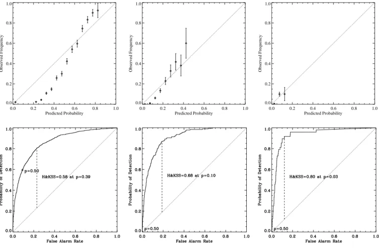
One way to visualize the H&KSS is to use a probability forecast to generate a Receiver Operating Characteristic (ROC) curve (Figure 2, left), in which the probability of detection (POD, first term on the right hand side of equa-tion (8)) is plotted as a function of the false alarm rate (FAR, second term on the right hand side of equation (8))
0.0 0.2 0.4 0.6 0.8 1.0 Predicted Probability 0.0 0.2 0.4 0.6 0.8 1.0 Observed Frequency
Figure 2. Example forecast verification plots for results using a sub-set of data (MCD#1, discussed in Section5) from one method (the machine-learning BBSO method, see §A.2), for the C1.0+, 24 hr event definition. Left: A Receiver Operating Characteristic (ROC) plot shows the probability of detection as a function of the false alarm rate by varying the threshold above which a region is predicted to produce a flare. Example thresholds withp∈[0.07,0.12,0.25,0.45,0.75] are labeled. In this case the maximum H&KSS occurs for p= 0.13, and is indicated by a dashed vertical line. Right: A reliability plot in which the observed frequency of flaring is plotted as a function of the forecast probability. Perfect reliability occurs when all points lie on thex=yline. For this case, there is a slight tendency to overprediction (i.e., points lying below and to the right of thex=y) in the three largest probability bins. The error bars are based on the sample sizes in each relevant bin.
by varying the probability threshold above which a region is predicted to flare. When the threshold is set to one, all regions are forecast to remain flare quiet, hence TP = FP = 0, which corresponds to the point (0,0) on the ROC diagram; when the threshold is set to zero, all regions are forecast to flare, hence FN = TN = 0, which corresponds to the point (1,1) on the ROC diagram. For perfect forecasts, the curve consists of line segments from (0,0) to (0,1) then from (0,1) to (1,1). A method that has an ROC curve that stays close to POD=1 while the FAR drops will be good at issuing all-clear forecasts; a method that has an ROC curve that stays close to FAR=0 while the POD rises will be good at forecasting events.
The flare forecasting methods discussed here generally predict the probability of a flare of a given class occurring, rather than a binary, categorical forecast. A measure of accuracy for probabilistic forecasts is the mean square error (MSE),
Aforecast= MSE(pf, o) =h(pf−o)2i (9)
where pf is the forecast probability, and o is the observed outcome (o= 0 for no event, o= 1 for an event). Perfect
accuracy corresponds to a mean square error of zero,Aperfect= 0.
TheBrier Skill Score(BSS) uses the climatological event rate as a reference forecast with a corresponding accuracy
Areference = MSE(hoi, o) (10)
thus
BSS = MSE(pf, o)−MSE(hoi, o)
0−MSE(hoi, o) . (11)
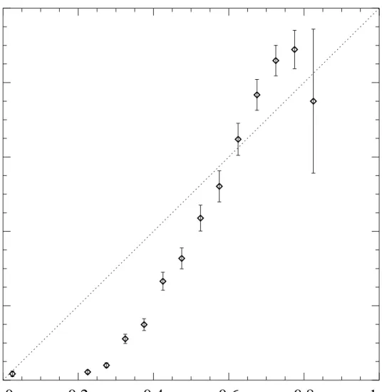
The Brier Skill Score can be complemented by a reliability plot, which compares the predicted probabilities with observed event rates, as demonstrated in Figure2, right. To construct a reliability plot, predicted probability intervals are selected, and the frequency of observed events within each interval is determined. This observed frequency is then plotted vs.the predicted probability, with error bars estimated based on the number of points which lie in each bin (e.g., Wheatland 2005). Predictions with perfect reliability lie along the x=y line, with observed frequency equal to predicted probability. Points lying above the line indicate underprediction while points lying below the line indicate overprediction. Perfect reliability isnot enough to guarantee perfect forecasts. For example, climatology has perfect reliability with a single point lying on thex=y line, but does not resolve events and non-events.
appropriate metric such as a skill score, but also to estimate the uncertainty in the metric. For the present study, no systematic attempt was made to estimate the uncertainties. However, this has been done for several individual methods using either bootstrap or jackknife approaches (e.g.,Efron & Gong 1983). For the nonparametric discriminant analysis described in§A.5, a bootstrap method estimate of the one sigma uncertainties gives values of order±0.01, ±0.02, ±0.03 for the C1.0+, 24 hr, M1.0+, 12 hr, and M5.0+, 12 hr sets, respectively. Given these values, all skill scores are quoted to two decimal places. A “+0.00” or “-0.00” result signals that there was an extremely small value on that side of zero.
All the methods produce probabilistic forecasts, so it was necessary to pick a probability threshold to convert to the categorical forecasts needed for the binary, categorical skill scores presented here. That is, a threshold probability was selected such that any forecast probability over the threshold was considered to be a forecast for an event, and anything less was considered to be a forecast for a non-event. Bloomfield et al. (2012) found that for the Poisson method, the best H&KSS and HSS are typically produced by picking a threshold that depends on the ratio FN/FP, with FN/FP≈1 giving the best HSS, and FN/FP≈Nevent/Nno event giving the best H&KSS. A similar approach to
Bloomfield et al. (2012) of stepping through the probability threshold was followed for each combination of method, skill score and event definition using the optimal data set for that method to determine the value that produced the maximum skill score. The Tables in AppendixAinclude the probability thresholds used, and ROC plots are presented for each method, with the best H&KSS shown by selecting the appropriate threshold.
4. OVERVIEW OF PREDICTION METHODS
Each participant in the workshop was invited to make predictions based on the data set provided (§2), and the event definitions described (§2.2). Generally, forecasting methods consist of two parts: (1) parameterization of the observational solar data to characterize the target active region, such as calculating the total magnetic flux, the length of strong neutral lines, etc., and (2) a statistical method by which prior parameters or flaring activity is used to evaluate a particular target’s parameters and predict whether or not it is going to flare.
The data analysis used by the methods broadly falls into two categories: those which characterize the photosphere (magnetic field and/or continuum intensity) directly (§ A.2, A.3, A.4, A.5, A.6, A.7, A.9, A.11), and those which characterize the coronal magnetic field based on the photospheric magnetic field (§A.1,A.8). These are supplemented by an event statistics approach (§A.10), which uses only the past flaring history, and thus serves as a baseline against which to compare the other methods.
A variety of statistical methods are employed to produce the forecasts from the parameterizations. At one end of this spectrum are methods based on a McIntosh-like classification (McIntosh 1990) from which a historical flaring rate is employed as a look-up table. At the other end are sophisticated machine-learning techniques that generally do not employa prioriclassifications. It may be possible to improve forecasts by combining the parameterization used by one group with the prediction algorithm of another group, but for the results presented here, no such attempt is explicitly made.
For each method, a brief description is provided here, with a more detailed description and some summary metrics of the performance of each method on its optimal subset of the data given in AppendixA. A comparison of methods on common data sets is presented in Section5.
The Effective Connected Magnetic Field - M. Georgoulis, A.1
The analysis presented inGeorgoulis & Rust(2007) describes the coronal magnetic connectivity using the effective connected magnetic field strength (Beff). TheBeff parameter is calculated following inference of a connectivity matrix
in the magnetic-flux distribution of the target active region. From the distribution ofBeff, flare forecasts are generated
using Bayesian inference and Laplace’s rule of succession (Jaynes & Bretthorst 2003).
Automated Solar Activity Prediction (ASAP) - T. Colak, R. Qahwaji, A.2
TheAutomated Solar Activity Prediction (ASAP; Colak & Qahwaji 2008, 2009) system uses a feature-recognition system to generate McIntosh classifications for active regions from MDI white-light images. From the McIntosh classifications, a machine-learning system is used to make forecasts.
Big Bear Solar Observatory/Machine Learning Techniques - Y. Yuan,A.3
The method developed at NJIT (Yuan et al. 2010, 2011) computes three parameters describing an active region: the total unsigned magnetic flux, the length of the strong-gradient neutral line, and the total magnetic energy dissi-pation, followingAbramenko et al. (2003). Ordinal logistic regression and support vector machines are used to make predictions.
Total Nonpotentiality of Active Regions - D. Falconer,A.4
based on the presence of strong gradient neutral lines,W LSG2, and the total unsigned magnetic flux. A least-squares
power-law fit to the event rates is constructed as a function of these parameters, and the predicted event rate is converted through Poisson statistics to the probability of an event in the forecast interval. The rate-fitting algorithm is best for larger flares, and so no forecasts were made for the C1.0+, 24 hr events.
Magnetic Field Moment Analysis and Discriminant Analysis - K.D. Leka, G. Barnes, A.5
The NWRA moment analysis parameterizes the observed magnetic field, its spatial derivatives, and the character of magnetic neutral lines using the first four moments (mean, standard deviation, skew and kurtosis), plus totals and net values when appropriate (Leka & Barnes 2003a). The neutral line category includes a variation on theRparameter described in SectionA.6. Nonparametric Discriminant Analysis (NPDA; e.g.,Kendall et al. 1983;Silverman 1986) is combined with Bayes’s theorem to produce a probability forecast using pairs of variables simultaneously.
Magnetic Flux Close to High-Gradient Polarity Inversion Lines - C. Schrijver, A.6
Schrijver (2007) proposed a parameter R, measuring the flux close to high gradient polarity inversion lines, as a proxy for the emergence of current-carrying magnetic flux. For the results here, theR parameter was calculated as part of the NWRA magnetic field analysis (SectionA.5), but is also included in the parameterizations by other groups (e.g., SMART, see Section A.9), with slightly different implementations (see Section 5.3). For the results presented here, predictions usingRwere made using one-variable NPDA (SectionA.5).
Generalized Correlation Dimension - R.T.J. McAteer, A.7
The Generalized Correlation (akin to a fractal) DimensionDBC describes the morphology of a flux concentration
(active region) (McAteer et al. 2010). The generalized correlation dimensions were calculated for “q-moment” values from 0.1 to 8.0. For the results presented here, predictions with these fractal-related parameterizations were made using one-variable NPDA (SectionA.5).
Magnetic Charge Topology and Discriminant Analysis - G. Barnes, K.D. Leka, A.8
In a Magnetic Charge Topology coronal model (MCT;Barnes et al. 2005, and references therein), the photospheric field is partitioned into flux concentrations with each one represented as a point source. The potential field due to these point sources is used as a model for the coronal field, and determines the flux connecting each pair of sources. This model is parameterized by quantities such as the number, orientation, and flux in the connections (Barnes et al. 2005;Barnes & Leka 2006,2008), including a quantity,φ2,tot, that is very similar to Beff (SectionA.1). Two-variable
NPDA with cross-validation is used to make a prediction (SectionA.5,Barnes & Leka 2006).
Solar Monitor Active Region Tracker with Cascade Correlation Neural Networks - P.A. Higgins, O.W. Ahmed, A.9
The SMART2 code package (Higgins et al. 2011) computes twenty parameters, including measures of the area and flux of each active region, properties of the spatial gradients of the field, the length of polarity separation lines, and the measures of the flux near strong gradient polarity inversion lines R (Section A.6, Schrijver 2007) and W LSG2
(SectionA.4,Falconer et al. 2008). These parameters are used to make forecasts using the Cascade Correlation Neural Networks method (CCNN;Qahwaji et al. 2008) using the SMART-ASAP algorithm (Ahmed et al. 2013).
Event Statistics - M.S. Wheatland, A.10
The event statistics method (Wheatland 2004) predicts flaring probability for different flare sizes using only the flaring history of observed active regions. The method assumes that solar flares (the events) obey a power-law frequency-size distribution and that events occur randomly in time, on short timescales following a Poisson process with a constant mean rate. Given a past history of events above a small size, the method infers the current mean rate of events subject to the Poisson assumption, and then uses the power-law distribution to infer probabilities for occurrence of larger events within a given time. Three applications of the method were run for these tests: active region forecasts for which a minimum of five prior events was required for a prediction, active region forecasts for which ten prior events were required, and a full-disk prediction.
Active Region McIntosh Class Poisson Probabilities - D.S. Bloomfield, P.A. Higgins, P.T. Gallagher,
A.11
The McIntosh-Poisson method uses the historical flare rates from McIntosh active region classifications to make forecasts using Poisson probabilities (Gallagher et al. 2002;Bloomfield et al. 2012). The McIntosh class was obtained for each region on a given day by cross-referencing the NOAA region number(s) provided in the NOAA Solar Region Summary file for that day. Unfortunately, forecasts for the M5.0+, 12 hr event definition could not be produced by this approach because the event rates in the historical data (Kildahl 1980) were only identified by GOES class bands (i.e., C, M, or X) and not the complete class and magnitude.
A comparison is presented here of the different methods’ ability to forecast a solar flare for select definitions of an event (as described in Section 2.2). The goal is not to identify any method as a winner or loser. Rather, the hope is to identify successful trends being used to identify the flare-productivity state of active regions, as well as failing characteristics, to assist with future development of prediction methods. The focus is on the Brier skill score, since methods generally return probability forecasts, but the Appleman skill score is used to indicate the performance on categorical forecasts. The ApSS effectively treats each type of error (misses and false alarms) as equally important, and so gives a good overall indication of the performance of a method. In practice, which skill score is chosen does not greatly change the ranking of the methods, or the overall conclusions, with a few exceptions discussed in more detail below.
5.1. Data Subsets
The request was made for every method to provide a forecast for each and every dataset provided. Many methods, as alluded to in the descriptions in AppendixA, had restrictions on where it was believed they would perform reliably, and so each method did not provide a forecast in every case. The resulting variation in the sample sizes, as shown in the summary tables, is not fully accounted for in the skill scores reported (Section3), meaning that direct comparisons between methods with different sample sets is not reliable. Even the Hanssen & Kuipers’ skill score is not fully comparable among datasets if the samples of events and non-events are drawn from different populations, for example all regions versus only those regions with strong magnetic neutral lines.
To account for the different samples, three additional datasets are considered for performance comparison. The first is all data (AD), with an unskilled forecast (the climatology, or event rate) used if a method did not provide a forecast for that particular target. In this way, forecasts are produced for all data for all methods. However, this approach penalizes methods that produce forecasts for only a limited subset of data.
The second approach is to extract the largest subset from AD for which all methods provided forecasts. Two such maximum common datasets were constructed, one (MCD#1) for all methods except the event-statistics, while the second (MCD#2) which included the additional event-statistics restrictions imposed by requiring at least ten prior events. One method (MSFC/Falconer,§A.4) did not return results for C1.0+, 24 hr, so strictly speaking these should be null sets. However, for the purposes of this manuscript, that method was removed for constructing the MCDs for C1.0+, 24 hr. A drawback to the MCD approach arises for the methods that were trained using larger data samples, i.e. samples which included regions that were not part of the MCD. For methods that trained on AD, for example, many additional regions were used for training, while for methods with the most restrictive assumptions, almost all the regions used for training are included in MCD#1, hence the impact of using the maximum common datasets varies from method to method. In the case of MCD#1, where the primary restriction is on the distance of regions from disk center, this may not be a large handicap since the inherent properties of the regions are not expected to change based on their location on the disk, although the noise in the data and the magnitude of projection effects do change. However, for MCD#2, the requirement of a minimum number of prior events means the samples are drawn from very different populations. Foranymethod, training on a sample from one population then forecasting on a sample drawn from a different population adversely affects the performance of the method.
The magnitude of the changes in the populations from which the samples are drawn can be roughly seen in the changes in the event rates shown in Table 5.1. Between AD and MCD#1, the event rates change by no more than about 10%; between AD and MCD#2, the event rates change by up to an order of magnitude for the smaller event sizes such that MCD#2 for C1.0+, 24 hr is the only category with more events than non-events. The similarity in the event rates of AD and MCD#1 is consistent with the hypothesis that they are drawn from similar underlying populations. However, based on the changes in the event rates, it is fairly certain that MCD#2 is drawn from different populations than AD and MCD#1. Despite this difference, measures of the performance of the methods are presented for all three subsets to illustrate the magnitude of the effect and the challenge in making meaningful comparisons of how well methods perform.
Table 3. Sample Sizes of All Data (AD)vs. Maximum Common Datasets (MCDs)
Event Event No Event Event No Event Event No Event
List Event Rate Event Rate Event Rate
AD MCD#1 MCD#2
C1.0+, 24 hr 2609 10356 0.201 789 3751 0.174 249 128 0.660 M1.0+, 12 hr 400 12565 0.031 102 3162 0.031 70 220 0.241 M5.0+, 12 hr 93 12872 0.007 26 3633 0.007 21 270 0.072
5.2. Method Performance Comparisons
The Appleman and Brier skill scores for each method are listed for each event definition in Tables4-6, separately for each of the three direct-comparison data sets: All Data, Maximum Comparison Datasets #1 (without the event-statistics restrictions) and #2 (with the further restrictions from event event-statistics). As described in§3, the probability thresholds for generating the binary, categorical classifications used for calculating the ApSS were chosen to maximize the ApSS computed for each event definition using each method’s optimal data set (see AppendixA)6When a method
produces more than one forecast (e.g., the Generalized Correlation Dimension,§A.7, which produces a separate forecast for eachq value), the one with the highest Brier Skill Score is presented. Using a different skill score to select which forecast is presented generally results in the same forecast being selected, so the results are not sensitive to this choice. Recalling that skill scores are normalized to unity, none of the methods achieves a particularly high skill score. No method for any event definition achieves an ApSS or BSS value greater than 0.4, and for the large event magnitudes, the highest skill score values are close to 0.2. Thus there is considerable room for improvement in flare forecasting. The skill scores for some methods are much lower than might be expected from prior published results. This is likely a combination of the data set provided here not being optimal for any of the algorithms, and variations in performance based on the particular time interval and event definitions being considered.
In each category of event definition and for most data sets, at least three methods perform comparably given a typical uncertainty in the skill score, so there is no single method that is clearly better than the others for flare prediction in general. For a specific event definition, some methods achieve significantly higher skill scores. There is a tendency for the machine learning algorithms to produce the best categorical forecasts, as evidenced by some of the highest ApSS values in Tables 4-6, and for nonparametric discriminant analysis to produce the best probability forecasts, as evidenced by some of the highest BSS values.
For rare events, most of the machine learning methods (ASAP, SMART2/CCNN, and to a lesser degree BBSO) produce negative BSS values, even when the value of the ApSS for the method is positive. This is likely a result of the training of the machine learning algorithms, which were generally optimized on one or more of the categorical skill scores with a probability threshold of 0.5. The maximum H&KSS is obtained for a probability threshold that is much smaller than 0.5 when the event rate is low (Bloomfield et al. 2012). When a machine learning algorithm is trained to maximize the H&KSS with a threshold of 0.5, it compensates for the threshold being higher than optimal by overpredicting (see the reliability plots in AppendixA). That is, by imposing a threshold of 0.5 and systematically overpredicting, a similar classification table is produced as when a lower threshold is chosen and not overpredicting. The former results in higher categorical skill score values, but reduces the value of the BSS because the BSS does not use a threshold but is sensitive to overprediction. In contrast, discriminant analysis is designed to produce the best probabilistic forecasts and so it tends to have high reliability (does not overpredict or underpredict). This results in good BSS and ApSS values.
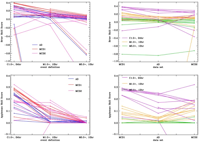
Skill scores from the different methods for the three data sets and different event definitions are shown in Figure3. Several trends are seen in the results. From the left panels, it can be seen that forecasting methods perform better on smaller magnitude events, whether evaluated based on the Brier or the Appleman skill score, with the most notable exceptions being ones for which the Brier skill score is negative for C1.0+, 24 hr, including the event statistics method. The event statistics method uses the small events to forecast the large events, and thus is not as well suited to
Figure 3. Skill scores from different methods for different data sets and different event definitions. Top: the Brier Skill Score and Bottom: the Appleman Skill Score as a function of the event definition (left) and the data set used (right). Not all methods produced forecasts for all event definitions and data sets, so a few points are missing from the plots. Several trends are clearly present in the results: methods generally perform better on smaller magnitude events, whether evaluated based on the Brier or the Appleman skill score, and most methods perform better on MCD#1 than on other datasets. The ranking of methods changes between the different data sets, showing the importance of using consistent data sets when comparing forecasting algorithms.
forecasting smaller events. The other exceptions are for the MCD#2, and thus are likely a result of a mismatch between the training and the forecasting data sets. The overall trend for most methods is likely due to the smaller sample sizes and lower event rates for the M1.0+, 12 hr and M5.0+, 12 hr categories, and holds for AD and both MCD sets. The smaller sample sizes make it more difficult to train forecasting algorithms, and the lower event rates result in smaller prior probabilities for an event to occur.
The right panels of Figure 3 show that almost all methods achieve higher skill scores on MCD#1 than on AD, although the improvement is modest. For methods that did not provide a forecast for every region, this is simply a result of the methods making better predictions than climatology. For methods providing a forecast for every region, it suggests that restricting the forecasts to close to disk center improves the quality of the forecasts, although the effect is not large. However, methods trained on AD and then applied to MCD#1 may show a more substantial improvement if trained on MCD#1. One of the main restrictions in many methods is the distance from disk center due to projection effects. Thus it is likely that improved results would be achieved by using vector magnetograms.
Most methods also achieve higher skill scores on MCD#2 than on AD, but a considerable fraction have lower skill scores, and there is more variability in the changes between AD and MCD#2, as measured by the standard deviation of the change in skill score, than in the changes between AD and MCD#1. This supports the hypothesis that AD and MCD#1 draw from similar populations, while MCD#2 draws from significantly different populations. The ranking of methods changes somewhat between AD and MCD#1, but more significantly between AD and MCD#2. This highlights the danger of using a subset of data to compare methods, particularly when the subset is drawn from a different population than the set used for training.
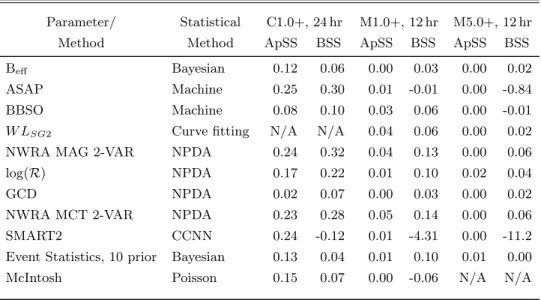
Table 4. Performance on All Data with Reference Forecast
Parameter/ Statistical C1.0+, 24 hr M1.0+, 12 hr M5.0+, 12 hr
Method Method ApSS BSS ApSS BSS ApSS BSS
Beff Bayesian 0.12 0.06 0.00 0.03 0.00 0.02
ASAP Machine 0.25 0.30 0.01 -0.01 0.00 -0.84
BBSO Machine 0.08 0.10 0.03 0.06 0.00 -0.01
W LSG2 Curve fitting N/A N/A 0.04 0.06 0.00 0.02
NWRA MAG 2-VAR NPDA 0.24 0.32 0.04 0.13 0.00 0.06
log(R) NPDA 0.17 0.22 0.01 0.10 0.02 0.04
GCD NPDA 0.02 0.07 0.00 0.03 0.00 0.02
NWRA MCT 2-VAR NPDA 0.23 0.28 0.05 0.14 0.00 0.06
SMART2 CCNN 0.24 -0.12 0.01 -4.31 0.00 -11.2
Event Statistics, 10 prior Bayesian 0.13 0.04 0.01 0.10 0.01 0.00
McIntosh Poisson 0.15 0.07 0.00 -0.06 N/A N/A
Note—An entry of N/A indicates that the method did not provide forecasts for this event definition.
Table 5. Performance on Maximum Common Dataset #1
Parameter/ Statistical C1.0+, 24 hr M1.0+, 12 hr M5.0+, 12 hr
Method Method ApSS BSS ApSS BSS ApSS BSS
Beff Bayesian 0.23 0.06 0.00 0.12 0.00 0.04
ASAP Machine 0.29 0.32 0.07 0.05 0.00 -0.81
BBSO Machine 0.24 0.30 0.12 0.17 0.00 -0.07
W LSG2 Curve fitting N/A N/A 0.14 0.24 0.00 0.10
NWRA MAG 2-VAR NPDA 0.30 0.38 0.08 0.16 0.00 0.07
log(R) NPDA 0.29 0.38 0.07 0.21 0.00 0.08
GCD NPDA 0.05 0.13 0.00 0.07 0.00 0.03
NWRA MCT 2-VAR NPDA 0.29 0.37 0.09 0.21 0.04 0.08
SMART2 CCNN 0.27 -0.22 0.03 -4.46 0.00 -12.49
Event Statistics, 10 prior Bayesian N/A N/A N/A N/A N/A N/A
McIntosh Poisson 0.12 -0.03 0.00 -0.05 N/A N/A
Note—An entry of N/A indicates that the method did not provide forecasts for this event definition.
Table 6. Performance on Maximum Common Dataset #2
Parameter/ Statistical C1.0+, 24 hr M1.0+, 12 hr M5.0+, 12 hr
Method Method ApSS BSS ApSS BSS ApSS BSS
Beff Bayesian 0.12 0.13 0.00 0.08 0.00 0.01
ASAP Machine 0.22 0.22 0.14 0.09 0.00 -0.72
BBSO Machine 0.23 0.17 0.17 0.11 0.00 -0.13
W LSG2 Curve fitting N/A N/A 0.19 0.18 0.00 0.08
NWRA MAG 2-VAR NPDA 0.38 0.29 0.11 0.08 0.00 0.04
log(R) NPDA 0.23 0.26 0.10 0.13 0.00 0.05
GCD NPDA -0.47 -0.37 0.00 -0.10 0.00 -0.02
NWRA MCT 2-VAR NPDA 0.23 0.25 0.11 0.10 0.05 0.04
SMART2 CCNN 0.15 0.18 0.03 -0.15 0.00 -1.47
Event Statistics, 10 prior Bayesian 0.05 -0.21 0.06 0.13 0.00 -0.03
McIntosh Poisson 0.02 -0.09 0.00 0.01 N/A N/A
Note—An entry of N/A indicates that the method did not provide forecasts for this event definition.
As discussed, different skill scores emphasize different aspects of performance. This is demonstrated by the results for the Beff and the BBSO methods shown in Table 5, for C1.0+, 24 hr using MCD#1. The forecasts using these
methods result in essentially the same values of the ApSS of 0.23 and 0.24, respectively. However, the corresponding BSS values of 0.06 and 0.30 are quite different. This is graphically illustrated in comparing Figure 4 with Figure2, right. TheBeff method (Fig.4) systematically overpredicts for forecast probabilities less than about 0.6, but slightly
underpredicts for larger forecast probabilities. Thus the probabilistic forecasts result in a small BSS, but by making a categorical forecast of an event for any region with a probability greater than 0.55, the method produces a much higher ApSS. The SMART/CCNN method produces a similar systematic under- and overprediction (see§A.9) while most methods (e.g., the BBSO method shown in Fig.2) have little systematic over- or underprediction, so the Brier and Appleman skill scores are similar.
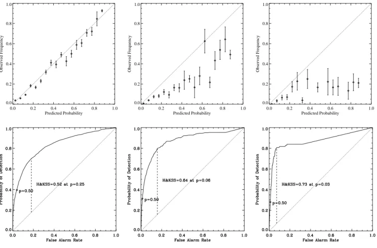
Inspection of reliability plots for a single method (Figure 5) shows a phenomenon common to most methods: the maximum forecast probability typically decreases with increasing event size, so most methods only produce low-probability forecasts for, say, M5.0+, 12 hr event definitions. This explains the small values of the Appleman skill score for larger event definitions as very few or no regions have high enough forecast probabilities to be considered a predicted event in a categorical forecast. It also suggests that all-clear forecasts have more promise than general forecasts. However, attention to the possibility of missed events would be critical from an operations point of view.
5.3. Differences and Similarities in Approach
All groups were given the same data, and many computed the same parameters. However, implementations differ significantly, so values for the same parameter are substantially different in some instances. In other cases, two parameters computed using completely different algorithms lead to parameter values that are extremely well correlated.
The total unsigned magnetic flux of a region,P
|Bz|, is often considered a standard candle for forecasting. Larger
regions have long being associated with greater propensity for greater-sized events, and the total flux is a direct measure of region size, hence it provides a standard for flare-forecast performance. Four groups calculated the total magnetic flux for this exercise, and provided the value for each target region. By necessity, since the MDI data provide only the line-of-sight component of the field vector, approximations were made, which varied between groups, and one group (NWRA) calculated the flux in two ways, using different approximations. There are also different thresholds used to mitigate the influence of noise, and different observing-angle limits beyond which some groups do not calculate this parameter. How large are the effects of these different assumptions and approximations on the inferred value of the total unsigned flux, and what is the impact on flare forecasting?
0.0
0.2
0.4
0.6
0.8
1.0
Predicted Probability
0.0
0.2
0.4
0.6
0.8
1.0
Observed Frequency
Figure 4. Reliability plot for the MCD#1, C1.0+, 24 hr forecasts based on Bayesian statistics and the Beff method, for
comparison with Figure2, right. The two forecasts have essentially identical Appleman skill scores, but very different Brier Skill scores.
Figure 5. Reliability plots for the BBSO predictions for (from left to right) the C1.0+, 24 hr, M1.0+, 12 hr, M5.0+, 12 hr event definitions and All Data treatment (reference forecast is used when no forecast was otherwise returned). Note the increasingly poor performance with event size and the increasing size of the error bars. This reflects the decreasing sample size for the larger events.
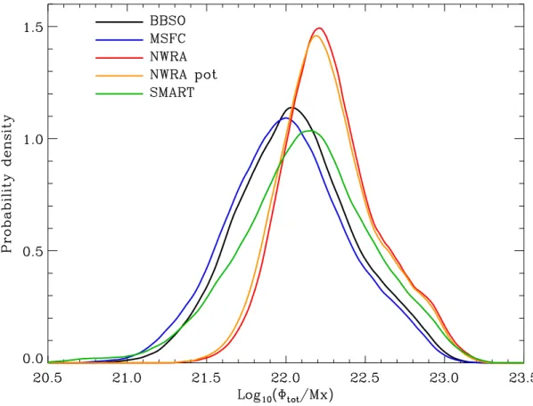
Figure 6. The distribution of the total unsigned flux, Φtot, as computed by different groups for the MCD#1. There are
considerable differences in both the width of the distribution and the location of its peak among the different implementations.
which includes the same regions. There are considerable differences among the distributions. In general, the NWRA values of the flux are larger than the other groups, although the SMART values have similar peak values, but with a tail to lower values than seen in the NWRA flux distribution. The NWRA distributions are also more sharply peaked than the other groups’ distributions.
To understand these differences, Figure7 shows the values for each group plotted versus the NWRA values, for all regions for which the flux was computed by that group. The NWRA method is used as the reference because it has a value for every region in the data set. The values for regions in the MCD#1 (black) generally show much less scatter than when all available regions are considered. However, there are systematic offsets in values for NWRA versus BBSO and MSFC even for the MCD#1. The MCD#1 only includes regions relatively close to disk center, so much of the scatter may be a result of how projection effects are accounted for. This is particularly apparent for the SMART values.
How much influence do the variations in the total flux resulting from different implementations have on forecasting flares? To separate out the effects of the statistical method, NPDA was applied to all of the total-flux related parameters. The forecast performance solely as a single-variable parameter with NPDA is summarized in Table 7. Because different approximations may not influence how well the determination of total flux works toward the limb, entries are included using both all data files (without restriction), and using only the maximum common dataset.
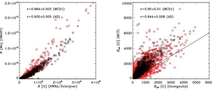
Figure 7. The total unsigned flux, Φtot, as computed by different groups, plotted as a function of Φtotcomputed by NWRA, with
the Pearson correlation coefficient shown in each plot. Black points are part of the MCD#1 used to compute the distributions in Figure 6, while red points are not. Although the values computed by some groups show strong correlation (e.g., BBSO and NWRA), others show only moderate (e.g., MSFC and NWRA) or weak correlations (e.g., SMART and NWRA). The correlations are stronger when considering only the MCD#1 points, indicating that most of the scatter is a result of the treatment of projection effects. In addition to scatter, there are systematic difference among the values from the different groups, even for the MCD#1 points.
Table 7. NPDA Forecasts from Total Flux, C1.0+, 24 hr
Group/ Appleman Skill Score Brier Skill Score
I.D. MCD#1 All Data MCD#1 All Data
BBSO 0.19±0.02 0.06±0.01 0.268±0.016 0.103±0.006 MSFC 0.19±0.02 0.13±0.01 0.265±0.015 0.182±0.008 NWRA Φlos 0.18±0.02 0.14±0.01 0.276±0.015 0.224±0.008
NWRA Φpot 0.18±0.02 0.18±0.01 0.276±0.014 0.246±0.008
Figure 8. Values of the same parameter obtained with different implementations. Left: a measure of the strong gradient polarity inversion lines, Rproposed bySchrijver(2007) as computed by two different groups. Right: a measure of the connectivity of the coronal magnetic field, Beff proposed byGeorgoulis & Rust (2007) as computed by two different groups. In both cases,
there are noticeable differences in the values of the parameter depending on implementation.
Despite differences in the inferred values of the total unsigned flux, the resulting skill scores for the MCD#1 are effectively the same for all the implementations. The AD forecasting results use a climatology forecast where a method did not provide a total flux measurement (because it was beyond their particular limits, for example). This difference can be seen in the variation between the results for AD and MCD#1, in particular for the BBSO implementation, which had the most restrictive condition on the distance from disk center for computing the total unsigned flux. Overall, the different implementations result in significantly different skill scores for AD.
There is also evidence that different approximations applied to the Blos to retrieve an estimate of Bz, the radial
field, can make a difference. The NWRA potential field implementation performs nearly as well on AD as on the MCD#1, and better than the other implementations on AD. This suggests that, for flare forecasting, the potential field approximation is better than theµ-correction when only measurements of the line of sight component are available. Details of the implementation are also important for other parameters. Figure8 illustrates the impact of imple-mentation on the measureRof the strong gradient polarity inversion lines proposed bySchrijver (2007), and on the measureBeff of the connectivity of the coronal magnetic field proposed byGeorgoulis & Rust(2007) as computed by
different groups. The difference is more pronounced in the connectivity measure. Although the same mathematical formula forBeff is used, the differences are due to the distinct approaches followed for partitioning a magnetogram to
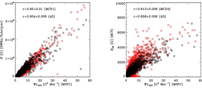
determine the point sources, and for inferring the connectivity matrix for a given set of sources, as noted in§A.8. In contrast to the differences in a parameter as implemented by different groups, parameters proposed by different researchers can also be strongly correlated. For example, the parameter Rproposed by Schrijver and the parameter W LSG2 proposed by Falconer are both measures of strong gradient polarity inversion lines. The methods by which
they are calculated are quite different, but the linear correlation coefficient between the two isr= 0.95 (Figure9, left). Perhaps even more surprising is thatW LSG2 is also strongly correlated with the parameterBeff ofGeorgoulis & Rust
(2007), which is a measure of the connectivity of the coronal magnetic field (Figure9, right).
Two conclusions can be drawn from this exercise. First, implementation details can greatly influence the resulting parameter values, although this makes surprisingly little difference in the forecasting ability of the quantities considered. Second, there may be a limited amount of information available for flare forecasting from only the line of sight magnetic field without additional modeling. Even if additional modeling is used, such as when the coronal connectivity is used to determineBeff, solar active regions that are small tend to be simpler, larger regions tend to be more complex, and
differentiating those with imminent flare potential remains difficult.
6. DISCUSSION AND SPECULATION
During the workshop and subsequent group discussions, a few salient points regarding flare forecasting methods emerged, and are discussed here.
Figure 9. Values of parameters characterizing different physical quantities. Left: two measures of the strong gradient polarity inversion lines,Rproposed bySchrijver(2007) andW LSG2proposed byFalconer et al.(2008). Right: theW LSG2 measure of
the strong gradient polarity inversion lines calculated by Falconer et al.(2008) and the Beff measure of the coronal magnetic
connectivity proposed byGeorgoulis & Rust(2007). Although these measures are based on different physical quantities, they are as strongly correlated as different implementations ofBeff (see Figure8, right).
Using NOAA ARs may be a less than optimal approach for forecasting. Sometimes there is no obvious photospheric division in the magnetic field of two NOAA ARs with clear coronal connectivity. Since the flux systems are physically interacting, they may be best treated as a single entity for the purpose of prediction. Yet identifying them thus can result in extremely large fractions of the Sun becoming a single forecasting target. Growing sunspot groups can occasionally be flare productive prior to acquiring a number by NOAA, and this will bias the results. Many groups are working on better active-region identification methods, but testing each is beyond the scope of this paper. Ideally, we would like to know where on the Sun a flare will occur, independent of the assignment of an active region number. The data used here were not ideal for any method. Each had different specific requirements on the data needed for a forecast, and it was difficult to accommodate these needs. Only by inserting a reference forecast when methods did not provide one, or by restricting the comparisons to the maximum common datasets, which relied upon only data for which all methods could provide forecasts, could a systematic comparison be made. For most combinations of event definition and data set, the best three methods resulted in comparable skill scores, so that no one method was clearly superior to the rest, and even which three methods resulted in the highest skill scores varied with event definition and data set. This result emphasizes that comparison of reported skill scores is impossible unless the underlying data, limits, treatment of missing forecasts, and event rates, are all standardized. Ideally, a common data set should be established in advance, such that all methods can train and forecast on exactly the same data, thus circumventing many of the difficulties in making a comparison.
There is a limit to how much information is available in a single line-of-sight magnetogram. Many of the param-eters used by different methods and groups are correlated with each other, meaning that they bring no independent information to the forecasts. More concerning is that parameter calculation and implementation differences, for even such a simple quantity as the total magnetic flux in a region, can significantly change the value of the parameter. Surprisingly, this had only a minor effect on forecasting ability for the cases considered. The use of vector field data and prior flare history may improve forecast performance by providing independent information.
Defining an event based on the peak output in a particular wavelength band (GOES 1-8 ˚A) is not based on the physics of flares. The soft X-ray signature (and hence magnitude) is not a direct measure of the total energy released in a reconnection event (Emslie et al. 2012), yet the parameters presently being computed are generally measures of the total energy of an active region. Considering how the energy release is partitioned between particles, thermal heating and bulk flow may lead to improved forecasts for the peak soft X-ray flux. Likewise, defining the validity period for a forecast based on a time interval related to the Earth’s rotational period (12 hr or 24 hr for the results presented here) has no basis in the physics of flares. Studies looking at either longer (Falconer et al. 2014) or shorter (Al-Ghraibah et al. 2015) validity periods do not show a substantial increase in performance. Nevertheless, considering
the evolution of an active region on an appropriate time scale may better indicate when energy will be released and thus lead to improved forecasts.
The forecast of an all-clear is an easier problem for large events than providing accurate event forecasts because there must be sufficient energy present for a large event to occur. When no active region has a large amount of free energy, and particularly during times when no active region faces the Earth, geo-effective solar activity is low in general and the possibility of a large flare is lower still. The low event rate for large events does mean that it is relatively easy to achieve a low false alarm rate. Still, during epochs when regions are on the disk, the inability of the prediction methods (admittedly, tested on old data) to achieve any high skill score values is discouraging, and shows that there is still plenty of opportunity to improve forecast methods.
In summary, numerous parameters and different statistical forecast methods are shown here to provide improved prediction over climatological forecasts, but none achieve large skill score values. This result may improve when updated methods and data are used. For those who could separate the prediction process into first characterizing an active region by way of one or more parameters, and then separately using a statistical technique to arrive at a prediction, both parameters and predictions were collected separately. It may be possible to increase the skill score values by combining the prediction algorithm from one method with the parameterization from a different method. Nonetheless, this study presents the first systematic, focused head-to-head comparison of many ways of characterizing solar magnetic regions and different statistical forecasting approaches.
This work is the outcome of many collaborative and cooperative efforts. The 2009 “Forecasting the All-Clear” Workshop in Boulder, CO was sponsored by NASA/Johnson Space Flight Center’s Space Radiation Analysis Group, the National Center for Atmospheric Research, and the NOAA/Space Weather Prediction Center, with additional travel support for participating scientists from NASA LWS TRT NNH09CE72C to NWRA. The authors thank the participants of that workshop, in particular Drs. Neal Zapp, Dan Fry, Doug Biesecker, for the informative discussions during those three crazy days, and NCAR’s Susan Baltuch and NWRA’s Janet Biggs for organizational prowess. Workshop preparation and analysis support was provided for GB, KDL by NASA LWS TRT NNH09CE72C, and NASA Heliophysics GI NNH12CG10C. PAH and DSB received funding from the European Space Agency PRODEX Programme, while DSB and MKG also received funding from the European Union’s Horizon 2020 research and in-novation programme under grant agreement No. 640216 (FLARECAST project). MKG also acknowledges research performed under the A-EFFort project and subsequent service implementation, supported under ESA Contract number 4000111994/14/D/MPR. YY was supported by the National Science Foundation under grants ATM 09-36665, ATM 07-16950, ATM-0745744 and by NASA under grants NNX0-7AH78G, NNXO-8AQ90G. YY owes his deepest gratitude to his advisers Prof. Frank Y. Shih, Prof. Haimin Wang and Prof. Ju Jing for long discussions, for reading previous drafts of his work and providing many valuable comments that improved the presentation and contents of this work. JMA was supported by NSF Career Grant AGS-1255024 and by a NMSU Vice President for Research Interdisciplinary Research Grant.
REFERENCES
Abramenko, V. I. 2005, ApJ, 629, 1141
Abramenko, V. I., Yurchyshyn, V. B., Wang, H., Spirock, T. J., & Goode, P. R. 2003, ApJ, 597, 1135
Ahmed, O. W., Qahwaji, R., Colak, T., Higgins, P. A., Gallagher, P. T., & Bloomfield, D. S. 2013, SoPh, 283, 157 Al-Ghraibah, A., Boucheron, L. E., & McAteer, R. T. J. 2015,
A&A, 579, A64
Alissandrakis, C. E. 1981, A&A, 100, 197 Balch, C. C. 2008, Space Weather, 6, 1001 Barnes, G. 2007, ApJ, 670, L53
Barnes, G. & Leka, K. D. 2006, ApJ, 646, 1303 —. 2008, ApJL, 688, L107
Barnes, G., Leka, K. D., Schrijver, C. J., Colak, T., Qahwaji, R., Yuan, Y., Zhang, J., McAteer, R. T. J., Higgins, P. A., Conlon, P. A., Falconer, D. A., Georgoulis, M. K., Wheatland, M. S., & Balch, C. 2016, ApJ, in preparation
Barnes, G., Leka, K. D., Schumer, E. A., & Della-Rose, D. J. 2007, Space Weather, 5, 9002
Barnes, G., Longcope, D., & Leka, K. D. 2005, ApJ, 629, 561
Berger, T. E. & Lites, B. W. 2003, Sol. Phys., 213, 213 Bloomfield, D. S., Higgins, P. A., McAteer, R. T. J., &
Gallagher, P. T. 2012, ApJL, 747, L41
Boser, B. E., Guyon, I. M., & Vapnik, V. 1992, in Proceedings of the Fifth Annual Workshop on Computational Learning Theory, COLT 92 (ACM)
Boucheron, L. E., Al-Ghraibah, A., & McAteer, R. T. J. 2015, ApJ, 812, 51
Chang, C.-C. & Lin, C.-J. 2011, ACM Trans. Intell. Syst. Technol., 2, 27:1
Colak, T. & Qahwaji, R. 2008, SoPh, 248, 277 —. 2009, Space Weather, 7, 6001
Conlon, P. A., Gallagher, P. T., McAteer, R. T. J., Ireland, J., Young, C. A., Kestener, P., Hewett, R. J., & Maguire, K. 2008, Sol. Phys., 248, 297
Conlon, P. A., McAteer, R. T. J., Gallagher, P. T., & Fennell, L. 2010, ApJ, 722, 577
Cortes, C. & Vapnik, V. 1995, Mach. Learn., 20, 273 Crown, M. D. 2012, Space Weather, 10, 6006