Empirical likelihood based longitudinal studies

(1)

by

c

⃝

Tharshanna Nadarajah

A thesis submitted to the School of Gradate Studies in partial fulfillment of the requirements for the degree of Doctor of Philosophy.

Department of Mathematics and Statistics

Memorial University

April 2016

(2)

Abstract

In longitudinal data analysis, our primary interest is in the regression parameters for the marginal expectations of the longitudinal responses; the longitudinal correlation parameters are of secondary interest. The joint likelihood function for longitudinal data is challenging, particularly for correlated discrete outcome data. Marginal mod-eling approaches such as generalized estimating equations (GEEs) have received much attention in the context of longitudinal regression. These methods are based on the estimates of the first two moments of the data and the working correlation structure. The confidence regions and hypothesis tests are based on the asymptotic normal-ity. The methods are sensitive to misspecification of the variance function and the working correlation structure. Because of such misspecifications, the estimates can be inefficient and inconsistent, and inference may give incorrect results. To overcome this problem, we propose an empirical likelihood (EL) procedure based on a set of estimating equations for the parameter of interest and discuss its characteristics and asymptotic properties. We also provide an algorithm based on EL principles for the estimation of the regression parameters and the construction of a confidence region for the parameter of interest. We extend our approach to variable selection for high-dimensional longitudinal data with many covariates. In this situation it is necessary to identify a submodel that adequately represents the data. Including redundant variables may impact the model’s accuracy and efficiency for inference. We propose a penalized empirical likelihood (PEL) variable selection based on GEEs; the variable selection and the estimation of the coefficients are carried out simultaneously. We discuss its characteristics and asymptotic properties, and present an algorithm for op-timizing PEL. Simulation studies show that when the model assumptions are correct, our method performs as well as existing methods, and when the model is misspecified, it has clear advantages. We have applied the method to two case examples.

(3)

varman, in gratitude for their endless love, support, and encouragement.

(4)

Acknowledgements

First, I would like to express my sincere gratitude to my advisor Dr. Asokan Mulayath Variyath, for his patience, enthusiasm, motivation, and immense knowledge. He has provided constant support during my Ph.D. research and has guided me throughout the preparation of this thesis. I could not have had a better advisor and mentor for my Ph.D.

My co-advisor, Dr. J. Concepci´on Loredo-Osti, has always been there to listen and offer advice. I am also thankful to him for encouraging the use of correct grammar and consistent notation and for carefully reading countless versions of this manuscript.

I gratefully acknowledge the financial support in the form of graduate fellow-ships and teaching assistantfellow-ships provided by Memorial University of Newfoundland’s School of Graduate Studies, the Department of Mathematics & Statistics, and my su-pervisor. I wish to thank all the faculty in our department for their support. It would not have been possible for me to complete the requirements of the graduate program without their guidance.

I would also like to thank my family, and in particular my wife and son, for their unwavering support in every way possible.

Finally, to my friends, thank you for your understanding and assistance during many, many moments of crisis. Your friendship enriches my life. I cannot list all your names here, but you are always on my mind.

(5)

List of tables

1.1 A class of stationary AR(1) correlation model for longitudinal count data. . . 9 1.2 Coverage probabilities of regression estimates for data from an AR(1)

cor-relation model under different working corcor-relation models (m=5). . . 10 1.3 Performance measures for count data with stationary covariates (m=5) . . . 18 3.1 Coverage probabilities of regression estimates for count data with stationary

co-variates for the independent, AR(1), EQC, and MA(1) models. . . 56 3.2 Coverage probabilities of regression estimates for count data with stationary

co-variates when the working correlation is misspecified for an AR(1) model. . . 57

3.3 Coverage probabilities of regression estimates for over-dispersion of count data with stationary covariates for the independent, AR(1), EQC, and MA(1) models. . . 58 3.4 Coverage probabilities of regression estimates for count data with nonstationary

covariates for the independent, AR(1), and EQC models. . . 62 3.5 Coverage probabilities of regression estimates for over-dispersion count data with

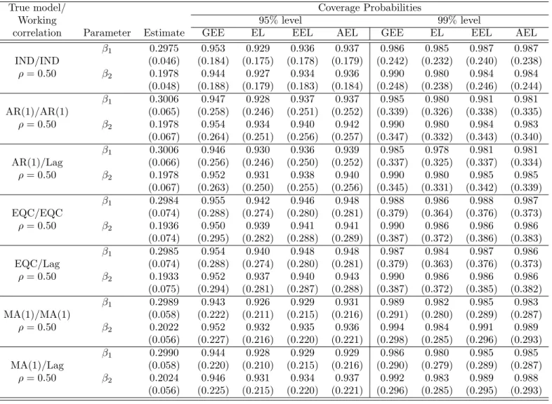
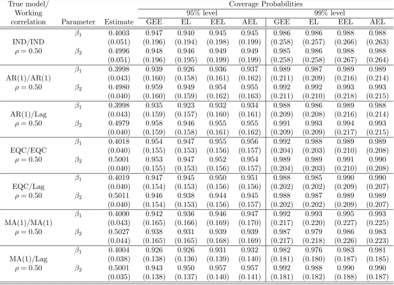
nonstationary covariates for the independent, AR(1), and EQC models. . . 67 3.6 Coverage probabilities of regression estimates for continuous data with stationary

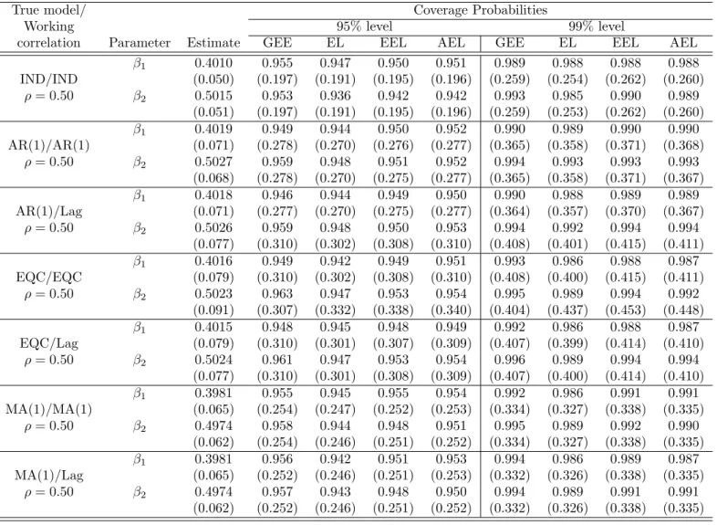
covariates for the independent, AR(1), EQC, and MA(1) models. . . 68 3.7 Coverage probabilities of regression estimates for continuous data with

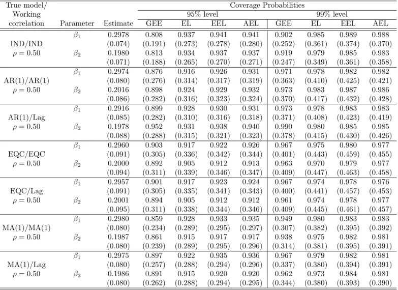
nonstation-ary covariates for the independent, AR(1), EQC, and MA(1) models. . . 69 3.8 Coverage probabilities of regression estimates for misspecified data with stationary

covariates for the independent, AR(1), EQC, and MA(1) models (k=50). . . 72 3.9 Coverage probabilities of regression estimates for misspecified data with

nonsta-tionary covariates for the independent, AR(1), EQC, and MA(1) models (k=100). . 73 4.1 Performance measures for count data with stationary covariates for the

(9)

EQC and MA(1) models. . . 89 4.3 Performance measures for count data with nonstationary covariates for the

inde-pendent, AR(1), and EQC models. . . 90 4.4 Performance measures for count data with stationary covariates when

the working correlation is misspecified for an AR(1) model. . . 91 4.5 Performance measures for count data with stationary covariates when

the working correlation is misspecified for the EQC model. . . 92 4.6 Performance measures for count data with stationary covariates when

the working correlation is misspecified for the MA(1) model. . . 93 4.7 Performance measures for over-dispersion count data with stationary

covariates for the independent and AR(1) models. . . 95 4.8 Performance measures for over-dispersion count data with stationary

covariates for the EQC and MA(1) models. . . 96 4.9 Performance measures for over-dispersion count data with nonstationary covariates

for independent, AR(1), and EQC models. . . 97 4.10 Performance measures for continuous data with stationary covariates

for the independent and AR(1) models. . . 98 4.11 Performance measures for continuous data with stationary covariates

for the EQC and MA(1) models. . . 99 4.12 Performance measures for continuous data with nonstationary

covari-ates for the independent and AR(1) models. . . 100 4.13 Performance measures for continuous data with nonstationary

covari-ates for the EQC and MA(1) models. . . 101 4.14 Performance measures for misspecified continuous data with stationary

covariates for the independent and AR(1) models. . . 102 4.15 Performance measures for misspecified continuous data with stationary

covariates for the EQC and MA(1) models. . . 103 4.16 Performance measures for misspecified continuous data with

nonsta-tionary covariates for the independent and AR(1) models. . . 104 4.17 Performance measures for misspecified continuous data with

nonsta-tionary covariates for the EQC and MA(1) models. . . 105 5.1 Regression estimates for health care utilization count data. . . 107

(10)

ferent working correlation structures. . . 109 5.3 PEL regression estimates for health care utilization data under different

working correlation structures. . . 109 5.4 Estimated coefficients for CD4 data set using AR(1) working correlation.111 5.5 Estimated coefficients for CD4 data set using EQC working correlation. 112 5.6 Estimated coefficients for CD4 data set using lag working correlation. . 113 5.7 Penalized variable selection for CD4 cell count data under different

working correlation structures. . . 113

(11)

List of figures

2.1 Construction of confidence interval using bisection. . . 49 5.1 Evolution of CD4 cell count measurements with and without drug use. 111 5.2 Evolution of square root of CD4 cell count measurements with and

(12)

Chapter 1

Introduction

1.1

Longitudinal Data

Longitudinal studies are common in areas such as epidemiology, clinical trials, eco-nomics, agriculture, and survey sampling. These studies investigate inference for data that involve repeated observations of the same subject over periods of time. The main feature of longitudinal data is that the repeated responses for each subject will likely be correlated since they relate to the same individual and consequently share the same covariates at any given point in time. In longitudinal studies, we are interested in the changes in the responses over time as a function of the covariates, generally under the assumption that observations from different individuals are independent. For ex-ample, longitudinal studies are used to characterize growth and aging, to assess the effect of risk factors on human health, and to evaluate the effectiveness of treatments. To obtain an unbiased, efficient, and reliable estimate, we must properly model the correlation between the repeated responses for each individual. However, the mod-elling of correlation, especially when the responses are discrete, is a challenging task even if the responses are collected over equi-spaced time points. The major methods

(13)

used for the analysis of longitudinal data dealing with mixed effects, transitional, and marginal regression models and the generalized estimating equation (GEE) approach.

1.2

Analysis of Longitudinal Data

Mixed effects regression is probably the most widely used methodology for the anal-ysis of longitudinal data. The most common models are linear mixed effects models (LMMs), nonlinear mixed effects models (NLMMs), and generalized linear mixed ef-fects models (GLMMs). Mixed efef-fects models incorporate the correlation within the individual responses by introducing random effects. LMMs and NLMMs are appropri-ate only for continuous responses. However, in practice, many types of responses follow non-Gaussian distributions, and in these cases GLMMs are appropriate. A potential disadvantage of mixed effects models is that they rely on parametric assumptions, which may lead to biased parameter estimates when a model is misspecified. More-over, the estimation of the parameters is challenging when the random effects have a high dimension; it typically involves integrals that do not have an explicit form. In the absence of an analytical solution, Breslow and Clayton [1993] proposed the penalized quasi-likelihood (PQL) for the GLMM; it uses a Laplace approximation to find the marginal likelihood. However, the PQL often yields biased estimates of the regression parameters since the estimators of the variance components are biased, especially for discrete longitudinal data.

Generalized linear models (GLMs) often handle longitudinal data by assuming a Markov structure that incorporates the correlation-within-individual measurements in the transitional models. In these Markov structure based GLM models, the con-ditional distribution of each response is expressed as a function of the past responses and the covariates. These models are more difficult to apply when there are missing

(14)

data and the repeated measurements are not equally spaced in time. In addition, the interpretation of the regression parameters varies with the order of the serial correla-tion, and the regression parameter estimates are sensitive to the assumption of time dependence. Because of the aforementioned difficulties in modelling and performing inference, we focus on marginal models in this thesis.

1.3

Marginal Models

The key component of the marginal model is that the mean response at each time point depends on the covariates through a known link function. The longitudinal observations consist of an outcome random variable yit and a p-dimensional vec-tor of covariates xit, observed for subjects i = 1, . . . , k at a time point t, t = 1, . . . , mi. For the ith subject, let yi = (yi1, . . . , yimi)

T _{be the response vector, and} let Xi = (xi1,xi2, ...,xit, ...,ximi)

T _{be the} _m

i × p matrix of covariates. Marginal models assume that the conditional mean of the tth response depends only on xit: E(yit|Xi) = E(yit|xi1, . . . ,ximi) = E(yit|xit). However, this assumption does not hold

when the covariate effect is time-dependent. As a result, special care is required when fitting marginal models with time-varying covariates. Marginal models describe only the (marginal) means of the outcome variables, ignoring the correlation or covariance structure of longitudinal observations.

Marginal models for longitudinal data can be extended to the GLM framework. The marginal density of yit is assumed to follow an exponential family (McCullagh and Nelder [1989]) of the form

f(yit) = exp [(yitθit−a(θit))φ+b(yit, φ)], (1.1)

(15)

of regression effects ofxit onyit, anda(∗) and b(∗) are functions that are assumed to be known. The mean and variance of yit can be written

E(yit|xit) =a′(θit) = µit and Var(yit) =a′′(θit) =v(µit)φ, (1.2)

where φ is the unknown over-dispersion parameter and v(∗) is a known variance function. For simplicity, we set the nuisance scale parameterφ to 1 in Equation (1.1) for the rest of this thesis. Let Θ be the natural parameter space of the exponential family distributions presented in (1.1) and Θ◦the interior of Θ. Let{a′(θ)}be a three times continuously differentiable function with {a′′(θ)} > 0 in Θ◦. Also, let h(η) be a three times continuously differentiable function with h′(η)>0 in g(M)◦, where M

is the image of{a′(Θ◦)}.

When the responses are continuous, the correlation can be represented by the linear dependence among the repeated responses. However, in the absence of a convenient likelihood function for discrete data, there is no unified likelihood-based approach for marginal models. Since our main interest is in modelling the relationship between the covariates and the response, we will not precisely model within-subject correlation (McCullagh and Nelder [1989]). Assuming the existence of the first two moments, Wedderburn [1974] proposed a quasi-likelihood (QL) approach for independent data. This approach is widely used to estimate regression coefficients without fully specifying the distribution of the observed data.

1.3.1

Quasi-likelihood

When there is insufficient information about the data for us to specify a parametric model, QL is often used. We can then develop the statistical analysis without fully specifying the distribution of the observed data; we first concentrate on cases where

(16)

the observations are independent. We assume that the meanµit is a function of the covariates with the regression parametersβ and covariance diagonal matrixσ2_V(_µ

it). To construct the QL, we start by looking at a single componentyit of y. The QL for complete data is Q(µ;y) = k ∑ i=1 mi ∑ t=1 Q(µit;yit), where Q(µit;yit) = ∫ µit yit yit−t

σ2_V(_t₎dt. The QL estimating equations for the regression

parametersβ are obtained by differentiating Q(µ;y): k ∑ i=1 mi ∑ t=1 [ ∂a′(θit) ∂β (yit−a′(θit)) Var(yit) ] =0.

For instance, in the Poisson case Var(yit) =a′′(θit) =a′(θit) = µit = exp(xitβ). In the longitudinal setup, the components of the response vector y_i correspond to repeated observations of the same covariates for the same subject, and they are likely correlated. LetCi(ρ) be themi×mi true correlation matrix ofyi,i= 1, . . . , k, which is unknown in practice. Our primary goal is to estimate β after taking the longitudinal correlation Ci(ρ) into account. For a knownCi(ρ), the QL estimator of β under (1.1) is the solution of the score equation

g(y;β) = k

∑

i=1

XT_i AiΣ−i 1(ρ)(yi−µi) =0, (1.3)

where Ai = diag [a′′(θi1), ..., a′′(θit), ..., a′′(θimi)] and Σi(ρ) = A

1/2

i Ci(ρ)A 1/2

i is the true covariance ofy_i.

In real applications the true correlation structure is often unknown. Ignoring the correlation of the measurements for the same individual could lead to an inefficient estimate of the regression coefficients and an underestimate of the standard errors.

(17)

If the probability distribution of the response y_i is poorly characterized, then it is obvious that we cannot use the likelihood approach. Even if it is not of primary interest, the correlation among a subject’s repeated measurements must be taken into account for proper inference. The joint distribution of the correlated discrete responses may not have a closed form when the correlation is taken into account. To avoid specifying the joint distribution of correlated discrete responses, Liang and Zeger [1986] proposed the GEE approach, an extension of GLMs to longitudinally correlated data analysis using QL.

1.3.2

Generalized Estimating Equation Approach

The GEE approach is a semiparametric method where the estimating equations are derived without a full specification of the joint distribution of the observed data. This approach to estimating the regression parameters allows the user to specify any structure for the correlation matrix of the outcomesy_i.

Liang and Zeger [1986] introduced a “working” correlation structure based on the GEE approach to obtain consistent and efficient estimators for the regression parameterβ. They solved

g(β,αˆ(β)) = k

∑

i=1

XT_i A1_i/2R−_i 1( ˆα)A−_i 1/2(y_i−µ_i) =0, (1.4)

where Ai is an mi ×mi diagonal matrix with Var(µit) as the tth diagonal element and Ri( ˆα) is the mi ×mi working correlation matrix of the mi repeated measure-ments used for Ci(ρ) in Equation (1.3). For j = 1, . . . , mi and j

′

= 1, . . . , mi, the (j, j′)th element of Ri is the known, hypothesized, or estimated correlation. The working correlation may depend on an unknown s×1 correlation parameter vector

(18)

but the correlation matrixRi(α) for theith subject is fully specified byα. The work-ing variance-covariance matrix for y_i is Var(α) = A_i1/2Ri(α)A

−1/2

i . Some common working correlation structures are independence, autoregressive of order one (AR(1)), equally correlated (EQC), moving average of order one (MA(1)), or unstructured. When Ri(α) = I in (1.4), the score equations are from a likelihood analysis, which assumes that the repeated observations from a subject are independent of one another. Liang and Zeger [1986] established the following properties of the estimator β

that satisfies g(βˆ,αˆ(β)) = 0 under the assumption that the estimating equation is asymptotically unbiased in the sense that limk→∞E[g(β₀,αˆ(β0))] =0,βˆis consistent,

and Cov(βˆ) can be consistently estimated. For a given working correlation structure,

αcan be estimated using a residual-based method of moments.

To improve the efficiency of the regression parameter estimates, Prentice and Zhao [1991] extended the GEE approach to allow for joint estimating equations for both the regression parameters β and the nuisance correlation parameters α. This approach needs the existence of the third and fourth moments of y_i, i= 1, . . . , k.

1.3.3

Limitations of GEE Approach

The GEE-based estimate ofβ is not necessarily consistent, as discussed by Crowder [1995] and Sutradhar and Das [1999]. Crowder [1995] demonstrated that in some situations the use of an arbitrary working correlation structure may lead to no solution for ˆα, which may break down the entire GEE methodology. Sutradhar and Das [1999] showed that the GEE approach may yield an estimator ofβ, that, although consistent, is less efficient than that of the independence estimating equation approach under an arbitrary working correlation structure. To overcome this difficulty, Sutradhar [2003] proposed using a stationary lag correlation structure instead of the working correlation matrix.

(19)

The estimate for β is obtained by solving the following estimating equations: g(β,ρˆ(β)) = k ∑ i=1 XT_i AiΣ−i 1(ρˆ)(yi−µi) =0, (1.5) where Σi( ˆρ) = A 1/2 i C ∗ i(ρ)A 1/2 i , with C ∗

i(ρ) the stationary lag correlation structure for the AR(1), MA(1), or EQC models, and

C∗_i(ρ) = ⎡ ⎢ ⎢ ⎢ ⎢ ⎢ ⎢ ⎢ ⎣ 1 ρ1 ρ2 . . . ρm−1 ρ1 1 ρ1 . . . ρm−2 . . . . ρm−1 ρm−2 ρm−3 . . . 1 ⎤ ⎥ ⎥ ⎥ ⎥ ⎥ ⎥ ⎥ ⎦ . (1.6)

The stationary lag correlations can be estimated via the method of moments intro-duced by Sutradhar and Kovacevic [2000]:

ˆ ρl= k ∑ i=1 m−l ∑ t=1 ˜ yity˜i,t+l/k(m−l) k ∑ i=1 m ∑ t=1 ˜ y_it2/km , (1.7)

wherel =|t−t′|, t≠ t′, t, t′ = 1, . . . , mand ˜yit is the standardized residual, defined as ˜

yit ={yit−µit}/{a′′(θit)}1/2. For an unequal number of time points, the correlation matrix given in (1.6) is estimated using the estimate of the lag correlationρl:

ˆ ρl = ∑k i=1 ∑m−l t=1 δitδi,t+ly˜ity˜i,t+l/ ∑k i=1 ∑m−l t=1 δitδi,t+l ∑k i=1 ∑mi t=1δity˜2it/ ∑k i=1 ∑mi t=1δit , (1.8)

(20)

wherem = max1≤i≤kmi, l = 1, . . . , m−1, and δiu= ⎧ ⎪ ⎪ ⎨ ⎪ ⎪ ⎩ 1, if u≤mi 0, if mi < u≤m.

Sutradhar and Das [1999] showed that the stationary lag correlation approach produces regression estimates that are consistent and more efficient than those ob-tained from the independence-assumption-based estimating equation approach. This approach assumes a known longitudinal correlation structure even though the corre-lation parameters are unknown.

We conducted a small simulation study to compare GEE with a stationary lag correlation approach when the correlation structure is misspecified. We consider a stationary correlation AR(1) model for longitudinal count data discussed by McKenzie [1988] and Sutradhar [2011]; see Table 1.1. We consider the stationary covariates ˜

xi = (˜xi1,x˜i2), where (˜xi1,x˜i2) is generated from the normal distribution with mean

0 and variance 1, and β = (0.3,0.2)T. For a given yi,t−1, ρ∗yi,t−1 is the binomial

thinning operation discussed by McKenzie [1988]. That is, ρ∗yi,t−1 = ∑ yi,t−1

j=1 bj(ρ) with Pr[bj(ρ) = 1] =ρ, Pr[bj(ρ) = 0] = 1−ρ. In our simulation we use m = 5 time points andk = 100 subjects. We simulated 1000 data sets with ρ= 0.49 and 0.70.

Model Dynamic Relationship Mean, Variance,

& Correlations AR(1) yit =ρ∗yi,t−1 +dit, t= 2, . . . , m E[yit] = ˜µi

yi1 ∼Poi( ˜µi = exp[˜xiβ]) Var[yit] = ˜µi

dit∼Poi[ ˜µi(1−ρ)], t= 2, . . . , m corr[yit, yi,t+l] =ρl =ρl

Table 1.1: A class of stationary AR(1) correlation model for longitudinal count data.

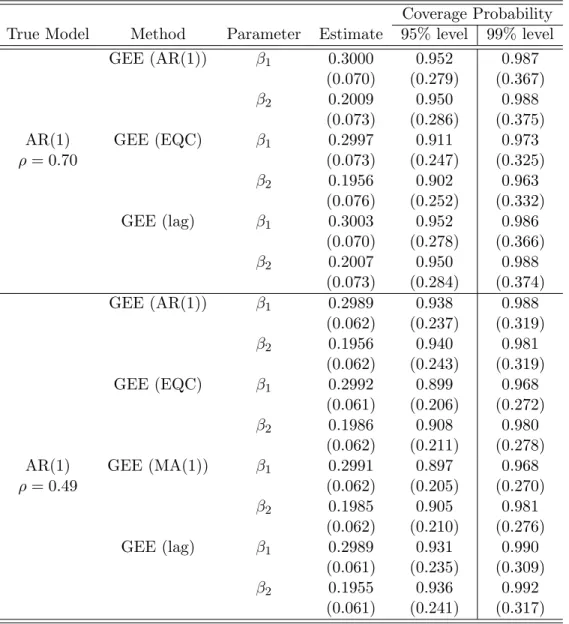
Table 1.2 gives the average estimated values of the regression coefficients and, in parentheses, the corresponding simulated standard errors. The table also gives the

(21)

coverage probabilities and the width of the confidence interval (CI) forβ1 and β2 for

the 0.95 and 0.99 confidence levels. We generated the data using an AR(1) correla-tion structure. We used AR(1), EQC, and MA(1) for the parameter estimacorrela-tion under GEEs, and we compared the results with those for GEEs with lag correlation. Table

Coverage Probability True Model Method Parameter Estimate 95% level 99% level

GEE (AR(1)) β1 0.3000 0.952 0.987 (0.070) (0.279) (0.367)

β2 0.2009 0.950 0.988 (0.073) (0.286) (0.375) AR(1) GEE (EQC) β1 0.2997 0.911 0.973

ρ= 0.70 (0.073) (0.247) (0.325) β2 0.1956 0.902 0.963 (0.076) (0.252) (0.332) GEE (lag) β1 0.3003 0.952 0.986 (0.070) (0.278) (0.366) β2 0.2007 0.950 0.988 (0.073) (0.284) (0.374) GEE (AR(1)) β1 0.2989 0.938 0.988 (0.062) (0.237) (0.319) β2 0.1956 0.940 0.981 (0.062) (0.243) (0.319) GEE (EQC) β1 0.2992 0.899 0.968 (0.061) (0.206) (0.272) β2 0.1986 0.908 0.980 (0.062) (0.211) (0.278) AR(1) GEE (MA(1)) β1 0.2991 0.897 0.968

ρ= 0.49 (0.062) (0.205) (0.270) β2 0.1985 0.905 0.981 (0.062) (0.210) (0.276) GEE (lag) β1 0.2989 0.931 0.990 (0.061) (0.235) (0.309) β2 0.1955 0.936 0.992 (0.061) (0.241) (0.317)

Table 1.2: Coverage probabilities of regression estimates for data from an AR(1) correlation model under different working correlation models (m=5).

1.2 shows that when we use the true working correlation structure, the coverage prob-abilities based on GEEs and GEEs with lag correlation are almost the same. However,

(22)

under an arbitrary working correlation structure, the GEEs with lag correlation have better performance. This indicates the loss of efficiency of the GEE estimators when the correlation structures are misspecified. We therefore recommend defining a lag correlation structure for the longitudinal responses.

The correlation structure (1.6) is quite robust, and it accommodates the AR(1), EQC, and MA(1) structures. Note, however, that the structure is unknown in prac-tice, and it is better to use a stationary lag-correlation structure to represent all three correlation structures. We did not consider all possible cases since some working corre-lation structure may lead to no solution for ˆα. For instance, under true exchangeable correlation with the MA(1) working correlation structure, the correlation parameter

ˆ

αdoes not exist.

The parameter β is defined by the estimating equations E[g(y;β)] = 0, where

g(y;β) ∈ Rr _{is an estimating function for} _β _{∈ R}p_{. When} _r ₌ _p _{the estimating} equations k−1∑k

i=1g(yi;β) = 0 have a unique solution for β. When r > p we have extra information about the parameter for improved efficiency, but it may not be possible to directly solve the estimating equations. To overcome this problem, Qu, Lindsay and Li [2000] proposed an adaptive quadratic inference function of the form

Q(β) =g′C−1_g_{, where}_g_{is a set of estimating functions based on moment assumptions}

and C is the estimated variance of g; this does not involve direct estimation of the correlation parameter. The above approaches are robust to the working correlation assumption. However, they are not robust to model misspecification.

(23)

1.4

Variable Selection for Longitudinal Data

Variable selection is an important issue in statistical modelling. It is especially im-portant for longitudinal data because of the high dimension of the explanatory vari-ables or predictors that arise in large-scale studies. A large number of predictors, (X1,X2, . . . ,Xp), are hypothesized to have an influence on the response variable y of interest. However, some predictors may have no influence or a weak influence, and may add noise to the estimation. Excluding these variables results in simpler model that may provide a better understanding of the underlying process.

Variable selection is the problem of identifying an optimal subset of predictor variables that adequately models the relationship between the response variable of interest and the predictors. The advantages of selecting a subset of the predictors are:

Simpler models are easier to interpret.

The predictive ability may be improved by eliminating irrelevant variables.

Removing redundant predictors reduces noise.

It is cheaper to measure fewer variables.

The main objective of variable selection is to identify the smallest adequate model. In GLMs, the submodel for a random variableywith mean µis a subset of components of X for which

g(x;µ)≃X(s)β(s)

where g(∗) is the link function, X(s) is a subset of the components of X, β(s) is a vector of the corresponding regression parameters, ands⊆(1,2, . . . , p). The variable selection problem is to find the best subset s such that the submodel is optimal according to some criteria that gives an adequate description of the data-generating mechanism.

(24)

Several variable selection methods for GLMs have been developed. Sequential ap-proaches such as forward selection, backward elimination, and the stepwise procedure are commonly used. These approaches are less computationally intensive than other methods, but the final model may not be optimal. The most widely used method for prediction models is the cross-validation approach (Stone [1974]). The resulting model may have a lower prediction error. However, in GLMs the concept of prediction error is not well defined (Fielding and Bell [2002]).

Two popular methods based on an information theoretic approach are Akaike’s information criterion (AIC), proposed by Akaike [1973, 1974], and the Bayesian infor-mation criterion (BIC), introduced by Schwarz [1978]. In these approaches, we need to evaluate all possible submodels and identify the best. A well-defined parametric model is necessary; if a parametric likelihood is not available, the empirical likelihood (EL) versions of AIC and BIC (Variyath, Chen and Abraham [2010]) can be used.

With high-dimensional data we cannot directly apply AIC or BIC because of the computational burden. Regularization methods have been developed to overcome the computational difficulties and to achieve selection stability. There is a large literature on the penalized likelihood approach, and two important approaches are the least ab-solute shrinkage and selection operator (LASSO; Tibshirani [1996]) and the smoothly clipped absolute deviation (SCAD; Fan and Li [2001]). Both approaches have many desirable properties. Related methods include penalized EL-based variable selection (Variyath [2006]; Nadarajah [2011]), adaptive LASSO (Zou [2006]; Zhang and Lu [2007]), least-square approximation (Wang and Leng [2007]), and the folded concave penalty method (Lv and Fan [2009]). Tang and Leng [2010] used a penalized EL framework, which is limited to mean vector estimation and linear regression models. The above methods are applicable only to GLMs.

(25)

Variable selection for longitudinal data is challenging because of the high dimen-sionality of the covariates and the need to construct a convenient joint likelihood function for correlated discrete outcome data. Pan [2001] developed the QL infor-mation criterion (QIC) under the working independence model and naive and robust covariance estimates of the estimated regression coefficients. Cantoni, Flemming and Ronchetti [2005] proposed a generalized version of Mallows’sCp, suitable for use with both parametric and nonparametric models. This approach avoids a stepwise proce-dure, and is based on a measure of the predictive error rather than on significance testing. Wang and Qu [2009] introduced a BIC-type procedure based on the quadratic inference function; it does not require the full likelihood or a QL. The implementa-tion of best-subset procedures requires the evaluaimplementa-tion of all possible submodels, which becomes computationally intensive when the number of covariates is large.

The idea of penalization is useful in longitudinal modelling and particularly in high-dimensional variable selection. Fan and Li [2004] proposed an innovative class of variable selection procedures for semiparametric models with continuous responses. Wang, Li and Huang [2008] studied regularized estimation procedures for nonparamet-ric varying-coefficient models with continuous responses; their procedures can simulta-neously perform variable selection and the estimation of smooth coefficient functions. Xiao, Zhang and Zhang [2009] investigated a double-penalized likelihood approach for selecting fixed effects in semiparametric mixed models with continuous responses. Dziak, Li and Qu [2009] discussed the application of a SCAD-penalized quadratic inference function. Xu, Wang and Zhu [2010] investigated a GEE-based shrinkage estimator with an artificial objective function. Xue, Qu and Zhou [2010] considered procedures for a generalized additive model where responses from the same cluster are correlated.

(26)

some of them are applicable only to continuous responses. To avoid specifying the full joint likelihood for correlated discrete data, Wang, Zhou and Qu [2012] proposed an approach based on penalized generalized estimating equations (PGEEs) with a nonconvex penalty function. This approach requires only the specification of the first two marginal moments and a working correlation matrix. In the next section, we will discuss PGEEs for variable selection in the context of longitudinal data analysis.

1.4.1

Penalized Generalized Estimating Equations

The approach of Wang et al. [2012] requires only the specification of the first two marginal moments and the correlation structure. This method provides computational efficiency and stability. It simultaneously performs the variable selection and the estimation of the regression parameters. That is, insignificant variables are removed by setting their regression parameters to zero. The method works reasonably well for high-dimensional problems.

In this method a penalized generalized estimating function is defined to be

U(β) = g(β,αˆ(β))−k∗p′_δ(|β|)sign(β), (1.9) whereg(β,αˆ(β)) =∑k i=1X T i A 1/2 i R −1 i ( ˆα)A −1/2

i (yi−µi) are the GEEs given in (1.4),

p′_δ(∗) is the first derivative of the penalty function, sign(β) = (sign(β1), . . . ,sign(βp))T with sign(t) = I(t > 0)−I(t < 0), and δ is the tuning parameter. Different penalty functions can be used. According to Fan and Li [2001], a good penalty function results in an estimator with the following three oracle properties:

1. Unbiasedness: The estimator is nearly unbiased when the true unknown param-eter is large.

(27)

coefficients to zero to reduce the model complexity.

3. Continuity: This property eliminates unnecessary variation in the model pre-diction.

A suitable penalty function is the SCAD penalty (Fan [1997]). Its first derivative is

p′_δ(θ) = δ

{

I(θ ≤δ) + (aδ−θ)+

(a−1)δ I(θ > δ)

}

for some a >2 and θ >0. (1.10)

Necessary conditions for the unbiasedness, sparsity, and continuity of the SCAD penalty have been proved by Antoniadis and Fan [2001]. This penalty function in-volves two unknown parameters, a and δ. Under some regularity conditions, Wang et al. [2012] show that the estimator based on the SCAD penalty satisfies the oracle properties for a certain choice ofa and δ.

PGEEs work reasonably well in high-dimensional problems, but the GEE ap-proach gives inconsistent estimators ofβunder an arbitrary working correlation struc-ture, and model misspecification limits the application of this method (see Section 1.3.3). Nadarajah, Variyath and Loredo-Osti [2016] developed penalized generalized QL (PGQL) variable selection based on the stationary lag correlation structure given in (1.6). We perform a simulation study to compare PGEEs and PGQL when the correlation structure is misspecified.

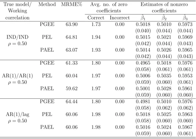
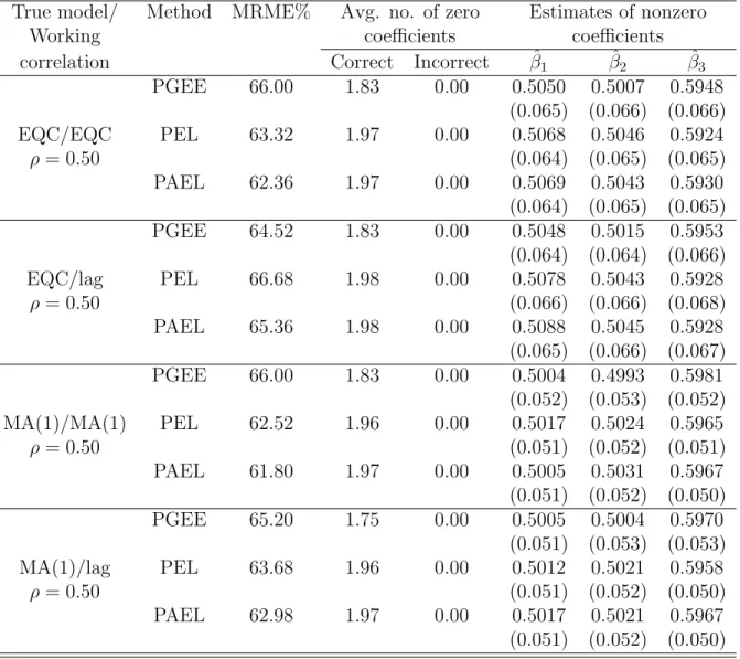
We consider the stationary AR(1) correlation model of Table 1.1. We use five covariates ˜Xi = (˜xi1, . . . ,x˜i5), where ˜xi1 ∼Bernoulli(0.5) andxi2 toxi5 are generated

from a multivariate normal distribution with mean zero, the correlation between xil and xjl is 0.5|i−j|, l = 2, . . . ,5. We set β = (0.5,0.5,0.6,0,0)T. We report (i) the median of the relative model error (MRME) and (ii) the average number of correct zero and nonzero coefficients. We also give the average estimated values of the nonzero coefficients and the corresponding simulated standard errors. The model error (ME)

(28)

is defined to be ME( ˆβ) = Ex

{

µ(Xβ)−µ(Xβˆ)}

2

, where µ(Xβ) = E(y|X), and the relative model error is RME = ME/MEfull, where MEfull is the model error when

fitting the data with the full model and ME is the model error of the selected model. We generated a sample with k = 100 individuals and m = 5 time points with three different correlation structures.

Table 1.3 shows that when we use the true working correlation structure, the MRME of the PGEEs is very close to that of PGQL. The average number of zero coefficients is close to the target of two, and the nonzero regression parameter esti-mates are close to the true values. However, under an arbitrary working correlation structure the PGEEs have a larger MRME, and the average number of zero coeffi-cients is not close to the target of two. When the working correlation is misspecified, PGQL performs better than the PGEEs. We repeated the simulation with different scenarios, and the conclusions were similar, so these results are omitted. However, the PGQL is not robust to misspecification. To handle possible misspecification of the mean, variance function, and correlation structure, a nonparametric method should be used.

1.5

Motivation and Proposed Approach for

Longi-tudinal Data Analysis

Marginal models or GEE approaches require only the specification of the first two marginal moments and a correlation structure. GEE estimators are consistent and asymptotically normal as long as the mean, variance, and correlation structure are correctly specified. Marginal models have satisfactory performance when the assump-tions are satisfied. Misspecification is a concern. Moreover, if the covariates are time-dependent the assumption limk→∞E[g(β0,αˆ(β0))] = 0 might not hold for an

(29)

True Model Method MRME% Avg. no. of zero Estimates of nonzero coefficients coefficients Correct Incorrect βˆ1 βˆ2 βˆ3 PGEE (IND) 86.86 1.25 0.0 0.5002 0.5023 0.5909 (0.068) (0.075) (0.076) PGEE (AR(1)) 65.60 1.85 0.0 0.5029 0.5058 0.5930 (0.066) (0.073) (0.071) AR(1) PGEE (EQC) 69.76 1.84 0.0 0.5030 0.5047 0.5935

ρ= 0.70 (0.066) (0.073) (0.072) PGQL 66.90 1.85 0.0 0.5034 0.5052 0.5930 (0.066) (0.073) (0.071) PGEE (AR(1)) 63.60 1.80 0.0 0.5003 0.5025 0.5968 (0.056) (0.056) (0.057) AR(1) PGEE (MA(1)) 70.57 1.65 0.0 0.5011 0.5021 0.5986

ρ= 0.49 (0.060) (0.061) (0.062) PGQL 67.64 1.79 0.0 0.5014 0.5029 0.5973 (0.059) (0.060) (0.061) PGEE (IND) 77.95 1.23 0.0 0.5059 0.5053 0.5913 (0.074) (0.076) (0.080) PGEEs (EQC) 61.43 1.87 0.0 0.5022 0.5066 0.5921 (0.073) (0.076) (0.074) EQC PGEE (AR(1)) 63.37 1.70 0.0 0.5025 0.5066 0.5914

ρ= 0.70 (0.074) (0.076) (0.076) PGQL 62.61 1.87 0.0 0.5026 0.5069 0.5916 (0.073) (0.076) (0.073) PGEE (EQC) 65.39 1.82 0.0 0.5023 0.5057 0.5922 (0.062) (0.065) (0.064) EQC PGEE (MA(1)) 75.50 1.59 0.0 0.4996 0.5022 0.5980

ρ= 0.49 (0.065) (0.068) (0.073) PGQL 66.40 1.82 0.0 0.5017 0.5046 0.5938 (0.064) (0.068) (0.069) PGEE (IND) 70.29 1.54 0.0 0.5002 0.5006 0.5994 (0.052) (0.054) (0.054) PGEEs (MA(1)) 63.56 1.72 0.0 0.5004 0.4993 0.5981 (0.052) (0.053) (0.052) MA(1) PGEE (AR(1)) 69.39 1.78 0.0 0.5018 0.5013 0.5963

ρ= 0.67 (0.052) (0.056) (0.054) PGEE (EQC) 71.37 1.71 0.0 0.5006 0.5008 0.5974 (0.052) (0.056) (0.058) PGQL 65.20 1.75 0.0 0.5005 0.5004 0.5970 (0.051) (0.053) (0.053)

Table 1.3: Performance measures for count data with stationary covariates (m=5)

arbitrary working correlation structure, and so the GEE estimate of β is not neces-sarily consistent; see Hu [1993], Pepe and Anderson [1994], Emond, Ritz and Oakes

(30)

[1997], Pan, Louis and Connett [2000], and Diggle, Heagerty, Liang and Zeger [2002]. The GEE estimator of β with the independent working correlation is always consis-tent so Pepe and Anderson [1994] recommended using this correlation as a safe choice. The independent working correlation is often efficient for the estimation of coefficients associated with time-independent covariates (Fitzmaurice [1995]). However, it may be much less efficient when the covariates are time-dependent (Fitzmaurice [1995]).

In practice, the true correlation structure is unknown, and using an arbitrary working correlation structure limits the application of marginal models. Misspecifica-tion can cause estimates based on marginal models to be inefficient and inconsistent, and inference in this situation can be completely inappropriate. Confidence regions and hypothesis tests are based on asymptotic normality, which may not hold since the finite-sample distribution may not be symmetric. These problems motivate us to investigate a nonparametric likelihood method. Instead of using marginal models, we define a subject-wise EL, based on a set of GEEs for the parameter of interest.

1.5.1

Proposed Approach to Longitudinal Data Analysis

Owen [1988] introduced the EL. The EL is a nonparametric method for statistical inference; that is, we need not assume that the data come from a particular distribu-tion. The EL combines the reliability of nonparametric methods with the flexibility and effectiveness of the likelihood approach. The EL has many nice properties parallel to those of parametric likelihood, including the ability to carry out hypothesis tests and construct confidence intervals without estimating the variance. The shape of EL confidence regions automatically reflects the emphasis of the observed data set. These regions are invariant under transformations and often behave better than confidence regions based on asymptotic normality when the sample size is small. The EL method also offers advantages in parameter estimation and the formulation of goodness-of-fit

(31)

tests. Moreover, it is possible to have more estimating equations than the number of parameters, i.e., r > p, where g(y;β) ∈ Rr _{is an estimating function for the} param-eter β ∈ Rp_{. For instance, let} _y

1, . . . , yn be independent and identically distributed univariate observations from a member of a semiparametric family F for which the first two moments are equal. If our aim is to estimateθ, the information aboutF is ex-pressed in the form of the estimating equationsg1(y, θ) =y−θ;g2(y, θ) = y2−θ−θ2.

In this example, r = 2 > p = 1. In this situation, we can estimate θ by maximizing the EL subject to the constraintE[g(y, θ)] = 0. The EL has been successfully applied in areas such as linear models, GLMs, survey sampling, variable selection, survival analysis, and time series.

We investigate the use of a nonparametric EL in longitudinal data analysis. We explore the asymptotic properties of the method and assess the performance of the method based on a large number of simulations. Our procedure provides consistent estimators, and has comparable performance to marginal models when the model assumptions are correct. It is superior to marginal models when the variance function and correlation structure are misspecified.

This result motivates us to extend the EL to the penalized EL-based variable se-lection with carrying out the estimation of the coefficients simultaneously. Simulation studies show that when the model assumptions are correct, its performance is com-parable to that of existing methods, and when the model is misspecified, our method has clear advantages.

1.6

Outline of Thesis

The main goal of this thesis is to explore longitudinal data analysis based on a non-parametric approach. We focus on the EL via a set of GEEs. In Chapter 2, we

(32)

develop the subject-wise EL via a set of GEEs of the parameter of interest, and discuss its characteristics and asymptotic properties. We also provide an algorithm based on EL principles for the estimation of the regression parameters and the con-struction of a confidence region for the parameter of interest. In Chapter 3 we present a performance analysis of our method in the context of count and continuous lon-gitudinal data. In Chapter 4, we extend this EL to penalized EL variable selection for high-dimensional longitudinal data. We discuss its characteristics and asymptotic properties, and provide an algorithm. We also present a performance analysis of the penalized EL variable selection in the context of count and continuous longitudinal data. In Chapter 5 we apply our method to two case examples. In Chapter 6 we provide concluding remarks, and discuss future research.

(33)

Chapter 2

Empirical Likelihood

The EL method is a powerful inference tool with promising applications in many areas of statistics. It is a nonparametric-likelihood-based approach, introduced by Owen [1988] that is an alternative to parametric likelihood and bootstrap methods. This method enables us to fully employ the information available from the data for making asymptotically efficient inference about the population parameters. In this chapter, we introduce the basic concept of EL for a mean vector and discuss EL-based longitudinal modelling.

2.1

Empirical Likelihood for Mean

For a given random sample y1, y2, . . . , yn from a known density f(y,µ), let L(µ) =

∏n

i=1f(yi,µ) be the likelihood function for the parameterµ, and let ˆµ= arg maxµL(µ)

be the maximum likelihood estimator. Suppose we wish to test the hypothesisH0 : µ=µ0.

Let

R(µ₀) = L(µ0)

(34)

be the likelihood ratio statistic. Wilks’ theorem (Wilks [1938]) states that under some regularity conditions−2 logR(µ₀) converges in distribution to a chi-square with degrees of freedom equal to the dimension ofµ.

Consider a random sample y1, y2, . . . , yn from an unknown distribution function

F(y) with pi = P r(Yi = yi), i = 1, . . . , n, where pi ≥ 0 and

∑n

i=1pi = 1. Since

P r(Y1 =y1, . . . , Yn=yn) =p1. . . pn, the likelihood function of F can be written

Ln(F) = n

∏

i=1

pi,

which is called an EL. The maximum EL estimator (MELE) forF gives an equal mass probability 1/n for the n observed values. The corresponding cumulative empirical distribution function ofy1, y2, . . . , yn is Fn(y) = 1 n n ∑ i=1 I(yi ≤y),

where I(∗) is the indicator function and the inequality is expressed componentwise. The log EL is of the form

ln(F) = n

∑

i=1

log(pi), (2.1)

subject to the constraints n

∑

i=1

pi = 1 and pi ≥0, i= 1,2, . . . , n.

Suppose that we are interested in the parameter µ=T(F) under the assumption that F is a member of a unknown distribution family F, for some functional T of the distribution. The purpose of the profile likelihood is to find the F at which the EL attains its maximum value over the set {F : T(F) = µ}. Define the profile EL

(35)

function to be

Ln(µ) = sup{Ln(F)| T(F) =µ, F ∈ F }.

We can make likelihood inference on µ based on Ln(µ). This likelihood has similar properties to its parametric counterpart. Since Ln(µ) ≤ n−n, it is convenient to standardizeLn(µ) by defining the likelihood ratio function to be

R(F) = nnLn(µ),

and it is easily shown that this can be written

R(F) = n

∏

i=1

npi.

To obtain confidence regions for µ= (µ1, µ2, . . . , µd), we define the profile empirical log-likelihood to be ℓ(µ) = sup { ln(F) : pi ≥0, i= 1,2, . . . , n; n ∑ i=1 pi = 1, n ∑ i=1 pi(yi−µ) = 0 } . (2.2)

We can computeℓ(µ) by maximizing ln(F) given in (2.1) as a constrained optimiza-tion problem using the Lagrange multiplier method. Making use of the first-order conditions of the Lagrangian function with respect to thepi and the constraint onpi, we see that the likelihood is maximized when

ˆ

pi =

1

n{1 + ˆλT(yi−µ)

(36)

and the Lagrange multiplier ˆλ= ˆλ(µ) is the solution of n ∑ i=1 (yi−µ) 1 +λT(yi−µ) =0.

Therefore, we can write the profile EL function as

ℓ(µ) =−nlog(n)− n

∑

i=1

log(1 + ˆλT(µ)(yi−µ)).

Consequently, the profile empirical log-likelihood ratio function becomes

W(µ) = n ∑ i=1 log(npˆi) = n ∑ i=1 log[1 + ˆλT(µ)(yi −µ) ] .

Owen [1990] showed that when µ₀ is the true population mean, 2W(µ₀) −→D χ2 d asn −→ ∞; similar to the parametric likelihood ratio function of Wilks [1938]. This result is useful for testing the hypothesisH0 :µ0 =T(F0) and for the construction of

100(1−α)% confidence regions, defined by

{

µ: 2W(µ)≤χ2_d(1−α)},

whereχ2_d(1−α) is the (1−α)th quantile of the chi-square distribution withddegrees of freedom. These are different from the CIs based on a normal approximation. Note that there is no need to estimate the scale parameters in the construction of the CI, and the confidence regions are not necessarily symmetric because of the data-driven approach. Because of these properties, the EL method has become popular in the statistical literature.

(37)

2.2

Empirical-Likelihood-Based Longitudinal

Mod-elling

Owen [1991] first considered the EL for linear models. EL confidence regions for regression coefficients in linear models were studied by Chen [1994]. The EL method can also be used to estimate the parameters defined by a set of estimating equations (Qin and Lawless [1994]). Owen [2001] provides a comprehensive overview of the EL and its properties. EL methods have attracted increasing attention over the last two decades, and the literature is extensive.

You, Chen and Zhou [2006] were the first to apply the EL to longitudinal data, using a subject-wise working independence model. This method ignores the within-subject correlation structure. Xue and Zhu [2007] proposed a within-subject-wise EL by centering the longitudinal data and obtained asymptotic normality of the MELE of the regression coefficients. They did not consider the within-subject correlation structure. It is well known that the working-independence assumption may lead to a loss of efficiency in estimation when within-subject correlation is present. Wang, Qian and Carroll [2010] showed how to incorporate the within-subject correlation structure of continuous repeated measurements into the EL. To estimate the within-subject covariance matrices, they used the nonparametric sample covariance matrix obtained from the residuals of a GEE using the working-independence assumption. In this thesis, we show how to incorporate the within-subject correlation structure of the repeated measurements into the EL.

We propose a subject-wise EL that assigns a probabilitypi to subjecti. For theith subject, lety_i = (yi1, . . . , yit. . . , yimi)

T _{be the response vector,}_X

i = (xi1,xi2, . . . ,ximi)

T

themi×pmatrix of covariates, andβ ∈ Rp the vector of the regression effects ofxon y. We assume that all the subjects are independent and the repeated measurements

(38)

yit taken on each subject are correlated.

Assuming the existence of the first two moments ofy, we can estimate the regres-sion parameters using the unbiased estimating equation

g(Yi;β,ρˆ(β)) = k

∑

i=1

X_iTAiΣ−i 1(ρˆ)(yi−µi) =0

as given in (1.5). Following Owen [1991] and Qin and Lawless [1994], we can extend the EL inference to longitudinal data based on a set of estimating functionsg(Y;β,ρˆ(β)). We incorporate the within-subject correlation structure of the repeated measurements into the EL using the well-known method of moments estimators given in (1.7) and (1.8) for a given value of β. The profile empirical log-likelihood function of β is defined by ℓ(β) = sup [ _k ∑ i=1 log(pi) : pi ≥0, i= 1,2, . . . , k; k ∑ i=1 pi = 1, k ∑ i=1 pigi(β,ρˆ(β)) = 0 ] .

The EL is maximized when

ˆ

pi =

1

k{1 + ˆλTgi(β,ρˆ(β))

}, i= 1,2, . . . , k, (2.3)

where the Lagrange multiplier ˆλ= ˆλ(β) is the solution of k ∑ i=1 gi(β,ρˆ(β)) 1 +λTgi(β,ρˆ(β)) =0. (2.4)

This result leads to the profile empirical log-likelihood function

ℓ(β) =−klog(k)− k

∑

i=1

(39)

and the profile empirical log-likelihood ratio function Wl(β) = − k ∑ i=1 log(kpˆi) = k ∑ i=1 log[1 + ˆλT(β)gi(β,ρˆ(β))]. (2.5)

Under some regularity conditions, we have 2Wl(β0) D −→χ2

p as k−→ ∞ if

E[g(β₀,ρˆ(β0))gT(β0,ρˆ(β0))

]

is full rank whereβ₀ is the true parameter value. This conclusion is similar to that for the parametric likelihood ratio function. The vectorβcan be estimated by minimizing

Wl(β) = k

∑

i=1

log(1 + ˆλT(β)g(β,ρˆ(β))) (2.6)

with respect toβ. Note that the profile log-likelihood ratio function can be minimized with respect toβ whenρis known. In practice, ρis unknown, but can be consistently estimated using the method of moments; see Section 1.3.3.

The computation of the profile EL function is a key step in EL applications, and it involves constrained maximization. In some situations, the algorithm may fail because of poor initial values of the parameters. Moreover, the poor accuracy of EL confidence regions has been reported by several authors, including Qin and Lawless [1994], Hall and La Scala [1990], Corcoran, Davison and Spady [1995], Owen [2001], Tsao [2004], and Chen, Variyath and Abraham [2008]. In the next subsection we will discuss how to address these problems in the context of longitudinal data.

(40)

2.2.1

Adjusted Empirical Likelihood

The computation of the profile EL ratio functionWl(β) given in (2.6) is a key step in EL applications. The solution for λ must satisfy {1 + ˆλT(β)gi(β,ρˆ(β))} > 0 for all

i= 1, . . . , k. A necessary and sufficient condition for its existence is that the vector

0 is an interior point of the convex hull of {gi(β,ρˆ(β)), i= 1, . . . , k}. Under some moment conditions on g(β,ρˆ(β)) (Owen [2001]), the convex hull contains 0 as an interior point with probability 1 ask → ∞. However, whenβ is not close to the true parameter valueβ₀ or whenk is small, it is possible that the solution of (2.4) does not exist. To avoid this problem, Chen et al. [2008] introduced the adjusted EL (AEL). The AEL is obtained by adding a pseudo-observation to the data set. It overcomes the difficulties arising when the estimating equations forλ have no solution.

Letgi(β) =gi(β,ρˆ(β)) andgk(β) = 1 k k ∑ i=1

gi(β) for any givenβ. For some positive constantbk, by the addition of an artificial observation

gk+1(β) =− bk k k ∑ i=1 gi(β)=−bkgk(β)

with bk = log(k)/2. The adjusted profile empirical log-likelihood ratio function is

W_l∗(β) = inf [ − k+1 ∑ i=1 log [(k+ 1)pi] :pi ≥0, i= 1,2, . . . , k+ 1; k+1 ∑ i=1 pi = 1, k+1 ∑ i=1 pigi(β) =0 ] = k+1 ∑ i=1 log[1 + ˆλT(β)gi(β) ]

with ˆλ = ˆλ(β) being the solution of k+1

∑

i=1

gi(β) 1 +λTgi(β)

=0. Note that 0 always lies inside the convex hull of{gi(β,ρˆ(β)), i= 1, . . . , k+ 1}. The adjusted profile empirical log-likelihood ratio function is well defined after adding a pseudo value gk+1(β). For

(41)

a wide range ofbk, following Chen et al. [2008], we can show that the adjusted profile EL ratio functionW_l∗(β) has the same asymptotic properties as the unadjusted profile EL ratio function Wl(β). We define the adjusted profile EL ratio estimator of β to be the minimizer of W_l∗(β) = k+1 ∑ i=1 [ log(1 + ˆλT(β)gi(β,ρˆ(β)) ] (2.7) with respect toβ.

The adjustment is particularly useful because, even for some undesirable values of

β, the algorithm guarantees a solution. The confidence regions constructed via the AEL are found to have better coverage probabilities than those for the regular EL, and the algorithm provides a promising solution for λ particularly when the sample size is small. The improved coverage probability is achieved without resorting to more complex procedures such as Bartlett correction or bootstrap calibration.

2.2.2

Extended Empirical Likelihood

One of the advantages of the EL is that we can use more information about the parameters. In other words, we can use more estimating equations than the number of parameters. The extra information should improve the accuracy of the estimates. In such cases, EL-based confidence regions can have undercoverage (Qin and Lawless [1994]). This is mainly because the parameter space is Rp_{, and the domain is a} bounded subset of Rp _{(Tsao [2013]; Tsao and Wu [2013]). This mismatch is a result} of the convex hull constraint set for the formulation of the EL. As a result, the values ofβ ∈ Rp_{that violate this constraint are excluded from the domain. To overcome this} problem, Tsao [2013] and Tsao and Wu [2013] expand the EL domain geometrically. This extended EL (EEL) for parameters based on estimating equations is a natural

(42)

generalization of the regular EL to the full parameter space. Similar to AEL, EEL have the same asymptotic properties as the EL.

For longitudinal data the EL domain is

Θk={β:β ∈ Rp such that k

∑

i=1

pigi(β,ρˆ(β)) = 0},

where g(β,ρˆ(β)) is given in (1.5). Tsao and Wu [2013] expand Θk to Rp through a composite similarity mappinghC

k : Θk → Rp. They define hCk(β) to be

hC_k(β) = ˜β+γ(k, Wl(β))(β−β˜), β ∈Θk, (2.8)

where ˜β is the MELE for β, and the function γ(k, Wl(β)) is the expansion factor, given by

γ(k, Wl(β)) = 1 +

Wl(β)

k .

Under the regularity conditions discussed by Tsao and Wu [2013], hC

k : Θk → Rp is surjective. Thus, s(β) = {β′ : hC

k(β ′

) = β}, ∀β ∈ Rp _{is nonempty. If} _s₍_β_{) contains} more than one point and hC_k does not have an inverse, then hC_k is surjective. Hence, a generalized inverseh−_kC : Rp _→_Θ

k is

h−_kC(β) = arg min

β′∈s(β)

{∥β′−β∥}.

The extended profile empirical log-likelihood ratio function W∗∗(β) under h−_kC is defined to be

W_l∗∗(β) =W(h_k−C(β)) for β ∈ Rp_,

which is well-defined throughout Rp_{. Tsao and Wu [2013] highlight the first-order} version of this EEL, which is easy to use and substantially more accurate than the

(43)

regular EL. It is also more accurate than available second-order EL methods. In our performance analysis in Chapter 3, we will explore the coverage probabilities based on the EEL, EL, and AEL.

In the next section, following Qin and Lawless [1994], we state and prove the results on the distributional properties of the adjusted profile EL estimates of βˆ. We construct these theorems based on the GEE with lag correlation given in (1.5), since the GEE estimate ofβ under an arbitrary working-correlation structure is not necessarily consistent; see Sections 1.3.3 and 1.4.1.

2.3

Distributional Properties

In this section, we present the first-order asymptotic properties ofβˆand the adjusted profile empirical log-likelihood ratio statistics. We first introduce some notation and regularity conditions that are used in the theorems and lemma.

Regularity Conditions:

A1: E{g(β₀,ρˆ(β0))}= 0, whereβ0is the true value ofβ,g(β,ρˆ(β)) =

∑k i=1D T i Σ −1 i (ρˆ)(yi−

µ_i) be the estimating function forβ∈ Rp_{(defined in (1.5)),} _D

i =∂{a′i(θ)}/∂β, Σi( ˆρ) =A 1/2 i C ∗ i( ˆρ)A 1/2

i , andAi = diag{a′′i(θ)}fori= 1,2, . . . , k. Letgk(β,ρˆ(β)) = 1

k

∑

i=1

gi(β,ρˆ(β)) andgk+1(β,ρˆ(β)) =−bkgk(β,ρˆ(β)), wherebk is a positive con-stant.

A2: {a′(θ)} is three times continuously differentiable and {a′′(θ)} >0 in Θ◦, where Θ be the natural parameter space of the exponential family distributions pre-sented in (1.1) and Θ◦ the interior of Θ. Also, h(η) is three times continuously differentiable and h′(η)>0.

(44)

A3: Eβ0 { ∂gk(β, ρ) ∂β } and Vk(β0,ρˆ(β0)) = Eβ0 { gk(β,ρˆ(β))gTk(β,ρˆ(β)) } are posi-tive definite.

A4: The rank of E

{

∂gk(β, ρ)

∂β

}

isp in a neighbourhood of β₀.

A5: There exist functionsG(y,X) such that in a neighbourhood ofβ₀.

⏐ ⏐ ⏐ ⏐ ∂gk(β, ρ) ∂β ⏐ ⏐ ⏐ ⏐ < G(y,X),∥gk(y,X,β,ρˆ(β))∥3 < G(y,X) with E[G(y,X)]<∞.

Lemma 2.3.1 Under regularity conditions A1-A5, suppose (y_i,Xi), i= 1,2, . . . , k is

a set of independent and identically distributed random vectors. Let

2W_l∗(β) = 2 k+1 ∑ i=1 log [ 1 + ˆλT(β)gi(β,ρˆ(β)) ] (2.9)

be the adjusted profile empirical log-likelihood ratio function. Then, as k → ∞, ρˆ(β)

is a consistent estimator in the neighbourhood of β; the correlation matrix of y_i is

C_i∗(ρ), defined in (1.5) and W_l∗(β) attains its minimum value at some point βˆ in

the interior of ∥βˆ−β₀∥ < k−1/3 _{in probability. In addition,} _β_ˆ _and _λ_ˆ₍_β₎ _{satisfy the}

equations Q1,k+1(βˆ,λˆ,ρˆ(β)) =0 and Q2,k+1(βˆ,λˆ,ρˆ(β)) =0 where Q1,k+1(β,λ, ρ(β)) = 1 k k+1 ∑ i=1 gi(β, ρ(β)) 1 +λT(β)gi(β, ρ(β)) , Q2,k+1(β,λ, ρ(β)) = 1 k k+1 ∑ i=1 1 1 +λT(β)gi(β, ρ(β)) ( ∂gi(β, ρ) ∂β )T λ. Proof of Lemma 2.3.1:

(45)

the repeated count responses which can be generalized for any repeated responses. Second, we are going to show that the Lagrange multiplier λ(β) = Op(k−1/3) for β such that ∥β−β0∥ ≤ k−1/3 and then going to show the consistency of the minimum

adjusted profile empirical likelihood ratio estimatorsβˆ.

Letyi1, . . . , yit, . . . , yim be the repeated count responses with the variance and the lag 1 covariance are given by

E(yit−µit)2 =σitt

and

E[(yit−µit)(yi,t+1−µi,t+1)] =σi,t,t+1 =ρµit+µitµi,t+1

respectively. Let ˜yit be the standardized residual, defined as ˜yit={yit−µit}/ √

σitt. Then it follows that

E [ _k ∑ i=1 m ∑ t=1 ˜ y2_it/km ] = 1 (2.10) and E [ _k ∑ i=1 m−1 ∑ t=1 ˜ yity˜i,t+1/k(m−1) ] =ρ k ∑ i=1 m−1 ∑ t=1 µit(σittσi,t+1,t+1)−1/2/k(m−1) + k ∑ i=1 m−1 ∑ t=1

µitµi,t+1(σittσi,t+1,t+1)−1/2/k(m−1). (2.11)

By using (2.10) and (2.11), we can write the first order approximate expectation

(46)

where w1 = k ∑ i=1 m−1 ∑ t=1 ˜ yity˜i,t+1/k(m−1) k ∑ i=1 m ∑ t=1 ˜ y2_it/km

is the lag 1 correlation as discussed in Section 1.3.3, and

h1 = k ∑ i=1 m−1 ∑ t=1 µit(σittσi,t+1,t+1)−1/2/k(m−1), and f1 = k ∑ i=1 m−1 ∑ t=1

µitµi,t+1(σittσi,t+1,t+1)−1/2/k(m−1).

We then obtain an approximate unbiased moment estimator ofρ

ˆ ρ= w1−f1 h1 . Now consider, E [( yit−µit √ σitt ) ( yi,t+1−µi,t+1 √ σi,t+1,t+1 )]

=σi,t,t+1(σittσi,t+1,t+1)−1/2 for all i and j.

That is, E [_m₋₁ ∑ t=1 ˜

yity˜i,t+1−σi,t,t+1(σittσi,t+1,t+1)−1/2

]

= 0 for alli= 1, . . . , k,

where ˜yit is the standardized residual. If µij’s and m are bounded, it is easy to see that E ⎡ ⎣ (_m₋₁ ∑ t=1 [ ˜

yity˜i,t+1−σi,t,t+1(σittσi,t+1,t+1)−1/2

] )2⎤

⎦< M

(47)

large numbers for independent random variable we can conclude that k ∑ i=1 m−1 ∑ t=1 [ ˜

yity˜i,t+l−σi,t,t+1(σittσi,t+1,t+1)−1/2

]

/k(m−1)−→P 0 as k → ∞.

Now, (2.11) can be written

k ∑ i=1 m−1 ∑ t=1 ˜ yity˜i,t+1/k(m−1) =ρ k ∑ i=1 m−1 ∑ t=1 µit(σittσi,t+1,t+1)−1/2/k(m−1) + k ∑ i=1 m−1 ∑ t=1

µitµi,t+1(σittσi,t+1,t+1)−1/2/k(m−1) +Op(1). (2.13)

Similarly, consider,

E[

˜

y_it2]

= 1 for alli and j.

That is, E [ _m ∑ t=1 ( ˜ y_it2 −1) ] = 0 for alli= 1, . . . , k.

Then ifµij’s and m are bounded,

E ⎡ ⎣ ( _m ∑ t=1 [ ˜ y_it2 −1] )2⎤ ⎦< M

for someM for alli= 1, . . . , k and y_i’s are independent. By the law of large numbers for independent random variable we can again conclude that

k ∑ i=1 m−1 ∑ t=1 [ ˜ y_it2 −1]/km−→P 0.

From this we can write

k ∑ i=1 m−1 ∑ t=1 ˜ y_it2/km= 1 +Op(1). (2.14)

(48)

By using (2.13) and (2.14), we can obtain w1(1 +Op(1)) = ρh1 +f1 +Op(1) ⇒ ˆ

ρ= w1−f1

h1

=ρ+Op(1) as k → ∞, where w1, f1, and h1 are defined in (2.12). So

ˆ ρ= w1−f1 h1 P −→ρ as k → ∞. (2.15) Let Vk(β,ρˆ(β)) = _k1 ∑k_i₌₁gi(β,ρˆ(β))giT(β,ρˆ(β)) and σ1k ≥ σ2k, . . . , σpk > 0 be eigenvalues of Vk(β0,ρˆ(β))). Without loss of generality, we assume σ1k →1. We will claim that ˆλ = Op(1). Let g∗(β,ρˆ(β)) = max1≤i≤k∥gi(β,ρˆ(β))∥. By condition A5,

g∗(β,ρˆ(β))≤max{G1/3₍_y i,Xi)

}

, i= 1,2, . . . , k+ 1 in the neighborhood of β₀. Following by Owen [2001] Lemma 11.2 (page 218), we obtain,g∗(β,ρˆ(β)) =Op(k1/3). We now consider the order of g_k(β,ρˆ(β)).

g_k(β,ρˆ(β)) = 1 k k ∑ i=1 gi(β,ρˆ(β)) = 1 k k ∑ i=1 gi(β0,ρˆ(β)) + 1 k(β−β0) k ∑ i=1 ∂gi(β∗,ρˆ(β)) ∂β ,

whereβ∗ is in the neighborhood ofβ₀.

By condition A1E[g(β₀,ρˆ(β))] =0 and V[g(β₀,ρˆ(β))]<∞, we have

g_k(β₀,ρˆ(β)) = 1 k k ∑ i=1 gi(β0,ρˆ(β)) = Op(k−1/2). (2.16)

Also by condition A5,

⏐ ⏐ ⏐ ⏐ ∂gi(β, ρ) ∂β ⏐ ⏐ ⏐ ⏐

< G(y,X) such that E[G(y,X)]<∞, we have

1 k k ∑ i=1 ∂gi(β∗,ρˆ(β)) ∂β =Op(1).

(49)

Therefore, uniformly in the region of∥β−β₀∥< k−1/3_{, we have}

g_k(β,ρˆ(β)) = Op(k−1/3).

Note that ˆλ(β) is the solution of the equation k+1 ∑ i=1 gi(β,ρˆ(β)) 1 +λT(β)gi(β,ρˆ(β)) =0. (2.17) Letξ=∥λ∥ˆ and ϑ= λ ξ. Multiplying (2.17) by ϑT k , we get 0= ϑ T k k+1 ∑ i=1 gi(β,ρˆ(β)) 1 +λT(β)gi(β,ρˆ(β)) = ϑ T k k+1 ∑ i=1 gi(β,ρˆ(β))− ξ k k+1 ∑ i=1 {ϑTgi(β,ρˆ(β))}2 1 +ξϑTgi(β,ρˆ(β)) . ≤ϑTg_k(β,ρˆ(β))(1−bk/k)− ξ k(1 +ξg∗₍_β_,_ρ_ˆ₍_β₎₎₎ k ∑ i=1 {ϑTgi(β,ρˆ(β))}2 . =ϑTg_k(β,ρˆ(β))− ξ k(1 +ξg∗₍_β_,_ρ_ˆ₍_β₎₎₎ k ∑ i=1 {ϑTgi(β,ρˆ(β))}2+Op(k−4/3bk). (2.18) Since 1 +ξg∗(β,ρˆ(β))≥0, we have ϑTg_k(β,ρˆ(β))≥ ξ k[1 +ξϑTg∗₍_β_,_ρ_ˆ₍_β_))] k ∑ i=1 {ϑT_g i(β,ρˆ(β))}2+Op(k−4/3bk).

For some 0< ϵ <1, the variance assumption on g(β,ρˆ(β)) in condition A3 gives 1 k k ∑ i=1 {ϑTgi(β,ρˆ(β))}2 ≥(1−ϵ)σ12k= (1−ϵ)

(50)

in probability. Therefore, as long as bk =op(k), (2.18) implies that ξ [1 +ξg∗₍_β_,_ρ_ˆ₍_β_))] ≤ϑ T g_k(β,ρˆ(β))× 1 (1−ϵ) =Op(k −1/3₎_.

From this, we can arrive ξ=Op(k−1/3) and hence λ(β) =Op(k−1/3). Next, 0= 1 k k+1 ∑ i=1 gi(β,ρˆ(β)) 1 +λT(β)gi(β,ρˆ(β)) = 1 k k+1 ∑ i=1 gi(β,ρˆ(β))− 1 k k+1 ∑ i=1 λT(β)[gi(β,ρˆ(β))gTi (β,ρˆ(β)) ] +op(k−1/3) =g_k(β,ρˆ(β))(1−bk/k)−λT(β)Vk(β,ρˆ(β))(1 +b2k/k) +op(k−1/3), (2.19)

where gk+1(β,ρˆ(β)) =−bkgk(β,ρˆ(β)) and bk is a positive constant. Hence, when

k→ ∞,

λ(β) =V−_k1(β,ρˆ(β))g_k(β,ρˆ(β)) +op(k−1/3). (2.20)

This result corresponds to Lemma 1 in Qin and Lawless [1994] which is about the consistency of maximum empirical likelihood estimates for independent and identically distributed data. By following Qin and Lawless [1994], under the regularity conditions A2-A5 and using (2.20), we can obtain, ask → ∞, with probability tending to 1 the equationsQ1,k+1(β,λ, ρ(β)) andQ2,k+1(β,λ, ρ(β)) has a solution within the open ball ∥βˆ−β₀∥< k−1/3_{. It is noted that rest of the proof is similar to the proof of Lemma 1}

in Qin and Lawless [1994] and the details are omitted here. This completes the proof.

Theorem 2.3.2 In addition to the regularity conditions A1-A5, suppose that ∂

2_g₍_β_{, ρ}₎

(51)