SEPARATION
Abd Majid Darsono
A thesis submitted to the Newcastle University for the degree of
Doctor of Philosophy
School of Electrical and Electronic Engineering
Faculty of Science, Agriculture and Engineering
SCHOOL OF ELECTRICAL AND ELECTRONIC
ENGINEERING
I, Abd Majid Darsono, confirm that this thesis and work presented in it
are my own achievement.
I have read and understand the penalties associated with plagiarism.
Signed:
ABSTRACT
Single channel source separation (SCSS) principally is one of the challenging fields in signal processing and has various significant applications. Unlike conventional SCSS methods which were based on linear instantaneous model, this research sets out to investigate the separation of single channel in two types of mixture which is nonlinear instantaneous mixture and linear convolutive mixture. For the nonlinear SCSS in instantaneous mixture, this research proposes a novel solution based on a two-stage process that consists of a Gaussianization transform which efficiently compensates for the nonlinear distortion follow by a maximum likelihood estimator to perform source separation. For linear SCSS in convolutive mixture, this research proposes new methods based on nonnegative matrix factorization which decomposes a mixture into two-dimensional convolution factor matrices that represent the spectral basis and temporal code. The proposed factorization considers the convolutive mixing in the decomposition by introducing frequency constrained parameters in the model. The method aims to separate the mixture into its constituent spectral-temporal source components while alleviating the effect of convolutive mixing. In addition, family of Itakura-Saito divergence has been developed as a cost function which brings the beneficial property of scale-invariant. Two new statistical techniques are proposed, namely, Expectation-Maximisation (EM) based algorithm framework which maximizes the log-likelihood of a mixed signals, and the maximum a posteriori approach which maximises the joint probability of a mixed signal using multiplicative update rules. To further improve this research work, a novel method that incorporates adaptive sparseness into the solution has been proposed to resolve the ambiguity and hence, improve the algorithm performance. The theoretical foundation of the proposed solutions has been rigorously developed and discussed in details. Results have concretely shown the effectiveness of all the proposed algorithms presented in this thesis in separating the mixed signals in single channel and have outperformed others available methods.
ACKNOWLEDGEMENT
Alhamdulillah. Thanks to Allah SWT, whom with His willing giving me the opportunity to complete this thesis.
This thesis is a collection of not only hard work, perseverance and continuous efforts in the past four years, but also encouragement, cooperation and support from many people. I would like to take an opportunity to acknowledge these people.
First and foremost, I would like to express my utmost gratitude to my primary supervisor Dr. Wai Lok Woo and second supervisor Profesor Satnam Dlay for giving me opportunity to pursue a PhD at Newcastle University. My deepest appreciation for my supervisors who nurtures me to become an independent researcher, trained me to critically analyse scientific issues and helped me understand concepts of signal processing. I am fortunate to have them as my supervisors who are never tired in giving me invaluable support, guidance and encouragement.
I would like also to extend my gratefulness to my research colleagues Bin Gao, Imran, and Norhaslinda who really helped me in giving me ideas and constructive suggestions for my research through our discussion.
I am also appreciated very much to my employer, Universiti Teknikal Malaysia Melaka (UTeM) and Ministry of Higher Education of Malaysia for their financial support for my study which made my research possible.
Last but not least, my deepest thankfulness goes to my beloved wife, Izwanni and my daughters, Nurin and Nura for their endless love, understanding, sacrifice, care and support. Thank you very much.
ABBREVIATIONS/ACRONYMS
SS Source Separation
BSS Blind Source Separation
SCSS Single Channel Source Separation CPP Cocktail Party Problem
CASA Computational Auditory Scene Analysis ICA Independent Component Analysis PCA Principal Component Analysis ISA Independent Subspace Analysis EMD Empirical mode Decomposition IMF Intrinsic Mode Functions GMM Gaussian Mixture Model
HMM Hidden Markov Model
FHMM Factorial Hidden Markov Model PNL Post-nonlinear
PDF Probability Density Function CDF Cumulative Density Function
TF Time-Frequency
FIR Finite Impulse Response
STFT Short Time Fourier Transform
LS Least Square
KL Kullback-Leibler
GMM Gaussian Mixture Model
NMF Nonnegative Matrix Factorization
NMF2D Two-Dimensional Nonnegative Matrix Factorization
SNMF2D Sparse Two-Dimensional Nonnegative Matrix Factorization FCNMF2D Frequency Constrained Two-Dimensional Nonnegative Matrix
Factorization
FC-SNMF2D Frequency Constrained Sparse Two-Dimensional Nonnegative Matrix Factorization
ML Maximum Log-likelihood
MAP Maximum a Posterior
Fro Frobenius Norm
IBM Ideal Binary Mask
WDO Windowed Disjoint Orthogonality SIR Signal-to-Interference Ratio SDR Signal-to-Distortion Ratio SAR Source-to-Artiacts Ratio PSR Preserved Signal Ratio
LIST OF CONTENTS
ABSTRACT……… ………...i ACKNOWLEDGEMENT………...ii ABBREVIATIONS/ACRONYMS……….iii LIST OF CONTENTS………..v LIST OF PUBLICATIONS………ix LIST OF FIGURES……….x LIST OF TABLES……….xiiiLIST OF SYMBOLS ………xiv
CHAPTER 1: INTRODUCTION………1
1.1 Background of Source Separation ...……….1
1.1.1 Source Separation Problem formulation ………2
1.1.2 Classification ……….3
1.1.2.1 Linear and Nonlinear SS ………....3
1.1.2.2 Instantaneous and Convolutive SS ………....4
1.1.2.3 Overdetermined and Undetermined SS ……….5
1.1.3 Application of source separation ………...…6
1.1.4 Single channel source separation ………...7
1.2 Objective of Thesis ………11
1.3 Thesis Outline ………12
1.4 Thesis Contributions ………..14
CHAPTER 2: LITERATURE OF SINGLE CHANNEL SOURCE SEPARATION ………...18
2.1 Model-based Statistical SCSS ………...20
2.2 Independent subspace analysis ………..23
2.3 Empirical Mode Decomposition ………26
2.4 Computational Auditory Scene Analysis ………...27
2.5 Nonnegative Matrix Factorization ……….31
2.5.1 Conventional NMF ………..32
2.5.2 Convolutive NMF ………34
2.5.3 Two-dimensional nonnegative matrix factorization …………36
2.6 Summary ………38
CHAPTER 3: NONLINEAR SINGLE CHANNEL SOURCE SEPARATION IN INSTANTANEOUS MIXTURE………...41
3.1 Background ………42
3.1.1 Nonlinear single channel instantaneous mixture ……….42
3.2 Proposed Separation Method ……….45
3.2.1 Nonlinearity compensation ………..45
3.2.2 Source Estimation: Maximum Likelihood ………...47
3.3 Results and Analysis ………..52
3.3.1 Experiment setup ………..52
3.3.2 Quality Evaluation ………52
3.3.3 Evaluation of proposed algorithm ………54
3.3.3.1 Gaussianization transform ………...54
3.3.3.2 Source separation result ………...57
3.3.3.3 Experiment using nonlinear handset model ………….60
3.4 Summary ………61
CHAPTER 4: LINEAR SINGLE CHANNEL SOURCE SEPARATION IN CONVOLUTIVE MIXTURE USING QUASI-EM AND MULTIPLICATIVE UPDATE FREQUENCY CONSTRAINED NONNEGATIVE MATRIX FACTORIZATION ………...62
4.1 Background ………65
4.1.1 Single channel convolutive mixture model ……….65
4.1.2 Itakura-Saito divergence properties ……….68
4.2 Proposed Separation Method………. 69
4.2.1 Source model ………...69
4.2.2 Formulation of Quasi-EM FCNMF2D ………72
4.2.2.1 Expressions of the E- and M-step ………73
4.2.2.2 Estimation of the spectral basis and temporal code…..75
4.2.3 Formulation of Multiplicative Update FCNMF2D…………..79
4.3 Results and Analysis ………..84
4.3.1 Feature extraction of toy data ………..85
4.3.2 Blind source separation ………89
4.3.2.1 Sources estimation ………...91
4.3.2.2 Comparison between Quasi-EM FCNMF2D and MU FCNMF2D ….………..92
4.3.2.3 Effect of frequency mixing, U ……….94
4.3.2.4 Separabilty analysis ……….96
4.4 Summary ………..100
CHAPTER 5: LINEAR SINGLE CHANNEL SOURCE SEPARATION IN CONVOLUTIVE MIXTURE USING FREQUENCY CONSTRAINED SPARSE NONNEGATIVE MATRIX FACTORIZATION ………102
5.1 Background ………..103
5.1.1 Two-dimensional sparse nonnegative matrix factorization... 103
5.2 Proposed Separation Method ………...105
5.2.1 Frequency constrained SNMF2D ………..106
5.2.2 Cost function with adaptive sparseness ……….106
5.2.3 Estimation of convolutive mixing, spectral basis and temporal code ………110
5.3 Results and Analysis ………117
5.3.1 Experiment setup ………...117
5.3.2 Evaluation of proposed algorithm ……….120
5.3.2.1 Estimated of spectral bases and temporal codes ……120
5.3.2.2 Source separation results ………...121
5.3.2.3 Adaptive behaviour of sparsity parameter ………….127
5.3.2.4 Impact of convolutive mixing, U ………...128
5.3.2.5 Convergence behaviour ……….130
5.3.3 Comparison between different cost function ……….131
5.3.4 Comparison with NMF-based method in convolutive mixture ………132
5.3.5 Experiment using live recorded sound ………...134
5.3.6 Experiment on professionally produced music recordings …137 5.4 Summary ………..140
CHAPTER 6: CONCLUSION AND FUTURE WORKS ………141
6.1 Summary and Contributions ………141
6.2 Future Works ………...144
6.2.1 Development of Nonlinear SCSS in Convolutive mixture …144 6.2.2 Development of EM Based Sparse NMF2D ………..145
LIST OF PUBLICATIONS
A.M. Darsono, Bin Gao, W.L. Woo, S.S. Dlay, “Nonlinear single channel source separation”, International Symposium on communications systems, networks and digital signal processing (CSNDSP 2010), 2010, pp: 507-511.
A.M. Darsono, Bin Gao, W.L. Woo, S.S. Dlay, “Sparsity aware machine learning algorithm for single channel convolutive source separation”, Submitted to IEEE Transaction on Systems, Man and Cybernetics, Part B: Cybernetics.
A.M. Darsono, Bin Gao, W.L. Woo, S.S. Dlay, “Frequency constrained nonnegative matrix factorization for single channel convolutive mixture”,
Submitted to IEEE Transaction on Neural Networks and Learning Systems. A.M. Darsono, Bin Gao, W.L. Woo, S.S. Dlay, “ Machine learning algorithm for
frequency-constrained nonnegative matrix factorization”, Submitted to 38th International Conference on Acoustics, Speech, and Signal Processing
LIST OF FIGURES
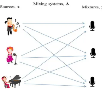
Figure 1.1: A simplified scenario of the source separation problem with three
audio sources and three microphones……….. 2
Figure 1.2: Single channel source separation problem where a single mixture of multiple sources is separated into their components………... 9
Figure 2.1: Schematic diagram of a general SCSS system……… 18
Figure 2.2: 3D-representation for W and H ……….. 37
Figure 3.1: Post-nonlinear mixing model for SCSS ………. 44
Figure 3.2: Proposed two-stage nonlinear SCSS ……….. 45
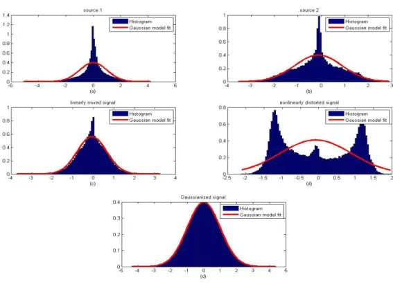
Figure 3.3: Histogram of (a) piano sound (b) flute sound (c) linearly mixed signal (d) nonlinearly distorted signal and (e) Gaussianized signal... 55
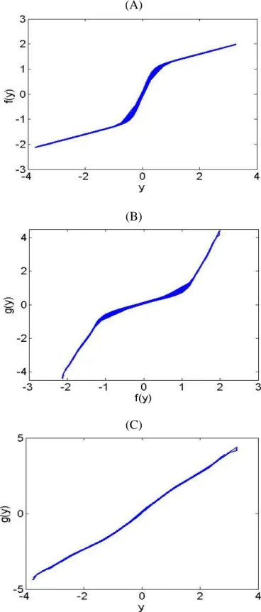
Figure 3.4: Scatter plot of (a) Nonlinear functions f(.) (b) Inverse function g(.)in relation to f(.) and (c) Gaussianized mixture……… 56
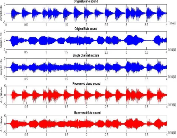
Figure 3.5: Separation results of nonlinear mixture using PNL algorithm……… 58
Figure 3.6: Separation results of nonlinear mixture using linear algorithm…….. 59
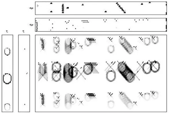
Figure 4.1: True factor of basis and code of the simulated convolutive mixed data………... 86
Figure 4.2: The estimated results using Quasi-EM FCNMF2D……… 86
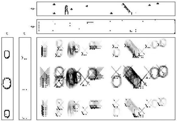
Figure 4.3: The estimated results using MU FCNMF2D………... 87
Figure 4.4: The estimated results using Quasi EM NMF2D (U=I)………... 87
Figure 4.5: The estimated results using MU NMF2D (U=I)………. 88
Figure 4.7: Log-frequency spectrogram of (A) piano, (B) trumpet and (C)
convolutive mixed signal………. 91 Figure 4.8: Separated sound in log-frequency spectrogram (A)-(B) piano and
trumpet sound using MU FCNMF2D (C)-(D) piano and trumpet
sound using Quasi-EM FCNMF2D………. 93 Figure 4.9: Separated sound in log-frequency spectrogram for the case of
without updating U (A)-(B) piano and trumpet sound using MU
NMF2D (C)-(D) piano and trumpet sound using Quasi-EM NMF2D 95 Figure 5.1: Time-domain representation and log-frequency spectrogram of
piano (top panels), trumpet (middle panels) and mixed signals
(bottom panels)………... 119
Figure 5.2: Estimated Wjand Hjfor (A) case (i), (B) case (ii), and (C) case (iii). 122 Figure 5.3: Separated signal in spectrogram. (A)-(B): piano and trumpet sound
for case (i). (C)-(D): piano and trumpet sound for case (ii). (E)-(F):
piano and trumpet sound for case (iii)………. 123 Figure 5.4: Separated signal in time domain (A)-(B): piano and trumpet sound
for case (i). (C)-(D): piano and trumpet sound for case (ii). (E)-(F):
piano and trumpet sound for case (iii)………. 124 Figure 5.5: Separation result of the sparsity parameter with different constant
value for j n, ……… 126 Figure 5.6: Trajectory of the sparsity parameters: (A) 0
1,1 , (B) 0 1,6 , (C) 0 1,11 and (D) 0 1,30 ……… 128
Figure 5.7: Separated piano and trumpet sound, respectively in TF domain using (A)-(B) Fixed Uj I (C)-(D) Proposed FC-SNMF2D……… 129 Figure 5.8: Evolution in log-log scale of the cost functions along the 1000
iterations of all 10 runs of the proposed algorithm……….. 131 Figure 5.9: Separation result in time domain. (A)-(B): Original piano and
trumpet. (C): Live recorded mixture of piano and trumpet sound.
(D)-(E): Separated piano and trumpet……….. 135 Figure 5.10: Separation result in time domain. (A)-(B): Original trumpet and
drum. (C): Live recorded mixture of trumpet and drum sound.
(D)-(E): Separated trumpet and drum……….. 136 Figure 5.11: Separation result in spectrogram for song “Make you feel my
love” by Adele. (A) music recording (B) estimated female vocal
(C) estimated piano sound……… 139 Figure 5.12: Separation result in spectrogram for song “You raised me up” by
Kenny G. (A) music recording (B) estimated saxophone sound
LIST OF TABLES
Table 3.1: Algorithm of two-stage nonlinear SCSS ………. 51
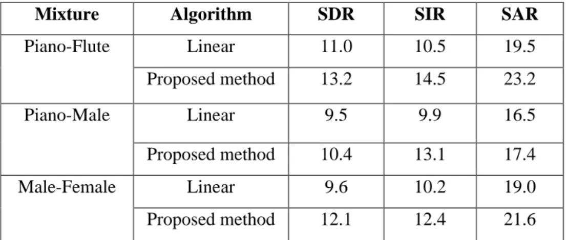
Table 3.2: Performance comparison of proposed method with linear algorithm in nonlinear mixture……… 59
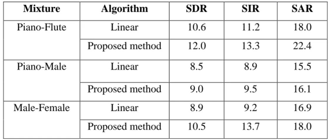
Table 3.3: Performance comparison using polynomial carbon-button nonlinearity………... 61
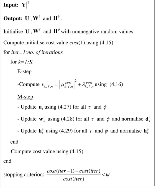
Table 4.1: Quasi-EM FCNMF2D algorithm……….. 79
Table 4.2: MU FCNMF2D algorithm……… 83
Table 4.3: Separation results for FCNMF2D methods……….. 94
Table 4.4: Separation results of proposed method with U=I………. 96
Table 4.5: Separability performance………... 100
Table 5.1: Proposed FC-SNMF2D algorithm……… 116
Table 5.2: Performance comparison between different sparsity methods (dB)…. 125 Table 5.3: Impact of U on separation performance………... 130
Table 5.4: Performance comparison between different cost functions…………. 132
Table 5.5: Performance comparison between different methods ……….. 134
Table 5.6: Source separation performances for various types of live-recorded audio mixture in terms of SDR (dB) ……… 137
LIST OF SYMBOLS
a Mixing parameter.
( )
m
c t mth intrinsic mode function (IMF) .
. ISC Itakura-Saito (IS) divergence cost function.
.KL
C Kullback-Leibler (KL) divergence cost function.
.LS
C Least square (LS) distance cost function. k
C kth component of the mixture.
e Noise.
E[.] Expectation.
f Frequency or frequency bin.
f(.) Nonlinear mixing function.
Fv(v) Cumulative density function (cdf) of v.
Fz(z) Cumulative density function (cdf) of z.
g(.) Inverse of f(.)
H Temporal code matrix.
H th slice of temporal code matrix.
j jth source. ICA
L Likelihood function of Independent Component Analysis (ICA)
m Mask.
ICA
m Basis function in ICA
iter
n Number of iterations. o
N Number of observed signals. s
N Number of independent sources.
.p Probability density function.
ML k
Q kth minus hidden-data log likelihood.
( ) EMD M
r t Final residue in empirical mode decomposition (EMD).
( )
j t
s Basis coefficient vector of source jth in ICA
Sa Amplitude similarity.
Sf Frequency similarity.
t Time or sample index.
u Mean vector.
U Frequency constrained of NMF2D ( )
v t Single channel of post-nonlinear mixture
k
V Posterior power of mixture component, Ck. ISA
w Time-varying weight in independent Subspace Analysis (ISA).
W Spectral basis matrix.
W thslice of spectral basis matrix.
,
f n
x Source signals in time-frequency (TF) domain.
x(t) Source signals in time domain.
.2
j
X Power spectogram matrix of jth source.
.2
im j
X Power spectogram matrix of j
th
,
f n
y Mixture or observation in time-frequency (TF) domain.
y(t) Mixture or observation in time domain.
.2
Y Power spectogram matrix of mixture y(t).
( )
z t Gaussianized time domain signal ISA
z Basis vector in independent Subspace Analysis (ISA).
Greek Symbols
Λ Sparsity parameters matrix
Sparsity parameter
post
Posterior variance
Σ Covariance matrix.
(. | .)
Gamma probability density function
( )
H m f
Cross spectrum of Hilbert spectrum.
( )
H m f
Spectral projection of Hilbert spectrum. θ Set of all parameter in estimation using EM.
Learning gain or learning rate.
(.)
Weighted Wiener filters. (.)
Cumulative density function of Gaussian. (.)
Gradient ascent adaptation of coefficient density.
post
Posterior mean
CHAPTER 1
INTRODUCTION
1.1 Background of Source Separation
Source separation (SS) has received wide attention and has been a topic of investigation for over two decades. SS problem refers to the statistical technique of separating a mixture of underlying source signals. Cocktail party problem (CPP) [1-2] is the classic example of SS problem to address the phenomenon associated with human auditory system that when a number of people are talking simultaneously with the present of background interferences and noise like in cocktail party, humans have the ability to focus their listening attention on a single speaker. During the last decade, many researchers and scientists have attempted to tackle this problem and remarkable developments have been achieved in the area of SS [3-12]. It has become one of the promising and exciting topics with solid theoretical foundations and potential applications in the fields of signal processing, neural computation and advanced statistics. SS has been successfully applied in various fields, such as speech enhancement, biomedical image processing, image processing, remote sensing, communication systems, exploration seismology, geophysics, econometrics, data mining and neural networks. Despite all these applications, so far there are no machines produced that can perform SS in the manner of human listening. It remains an open problem and demands further research investigation.
Figure 1.1: A simplified scenario of the source separation problem with three audio sources and three microphones
1.1.1 Source separation problem formulation
A general SS problem can be illustrated as in Figure 1.1 which is mathematically defined according to the conventional linear model as follows: A set of observations
T 1 2 ( ) ( ) ( ) ( ) o N t y t y t y t
y which are random processes is generated as a mixture of
underlying source signals ( ) 1( ) ( )1 ( ) T
s N t x t x t x t x according to: 11 12 1 1 1 2 21 22 2 2 1 2 ( ) ( ) ( ) ( ) ( ) ( ) ( ) ( ) s s o o o o s s N N N N N N N N a a a y t x t y t a a a x t t t y t a a a x t y Ax (1.1)
where A is the unknown mixing matrix of dimension NoNs and t is the time or sample index. The technique of SS aims to estimate both the original sources
T 1 1 ( ) ( ) ( ) ( ) s N t x t x t x t
x and the mixing matrix A using only the observations
T 1 2 ( ) ( ) ( ) ( ) o N t y t y t y t
y . It is noted that (1.1) represents a simplified model which may not be true representation of the real environment. In order to represent a realistic model, issues such as propagation delay of signals, nonlinear distortions, and noise should be taken into account and evaluated. Hence the need for further research has led to various branches of research in SS.
1.1.2 Classification of source separation
A literature review of current reports shows that there exist three main classifications of SS. These include: Linear and Nonlinear SS; Instantaneous and Convolutive SS; Overdetermined and Underdetermined SS.
1.1.2.1Linear and Nonlinear SS
Linear algorithms were a popular choice and dominate the SS research field because of its simplicity in analysis and its explicit separability. As defined in (1.1), linear SS assumes that the mixture is represented by a linear combination of source signals [3], [13]. Nevertheless, nonlinearity occurs in practical problems which leads to the issue of model mismatch [14-18] and this consequently led to the emergence of
models based on nonlinear SS. This model represent more accurate model of a realistic environment by taking nonlinear distorted signals into consideration.
A general nonlinear SS model can be expressed as:
( )t ( )t
y f x (1.2) where y( )t and x( )t are defined in (1.1) and f .
is the nonlinear mixing process. The nonlinear SS problem is more complicated than the linear SS problem because the principle of linear superposition of the source signals is violated. Under general nonlinear condition statistical independence is not sufficiently strong to recover the sources without any distortions and there always exist infinite solutions in nonlinear SS problems if the nonlinear mixing function f .
is not constrained [19]. Therefore, some form of constraints need to be imposed and nonlinear mixing models with constraints are generally preferred over a general model. An example of a constrained nonlinear model is the post-nonlinear model [20-22] which can be expressed as1 ( ) ( ) s N i i ij j j y t f a x t
(1.3) where fi
. is a nonlinear distortion function and1 ( ) s N ij j j a x t
is a linear mixing process.1.1.2.2Instantaneous and Convolutive SS
The convolutive mixture occurs when observed signals consist of combinations of multiple time-delayed versions of the original source signals and/or mixed signals themselves. Without the presents of time delays results in the instantaneous mixture
of observed signals which is expressed in (1.1). In linear convolutive mixture models, each element of the mixing matrix A in (1.1) becomes a filter instead of a scalar, which results in the observation signals represented by a linear combination of a set of time-delayed source signals, expressed as
11, 12, 1 , 1 1 1 2 21, 22, 2 , 2 0 1, 2, , ( ) ( ) ( ) ( ) ( ) ( ) ( ) ( ) s s o o o o s s N L N N N N N N N a a a y t x t y t a a a x t t t y t a a a x t
y A x (1.4)where A( ) is the finite-impulse response (FIR) of some causal filters and L-1 is the length of the filter. From (1.4), it can be seen that the simplest conventional linear instantaneous SS model can actually be considered as a special case of linear convolutive SS when A( ), 0 L 1 is reduced to A.
1.1.2.3Overdetermined and Undetermined SS
Overdetermined SS refers to the separation problem when the number of observed signals are more than the number of independent sources
No Ns
. On the other hand, when the number of observed signals is smaller than the number of independent sources
No Ns
, this becomes underdetermined SS. Overdetermined problem can be easily solved by reducing to determined SS as in (1.1). As for the underdetermined BSS [23-25], the separation quality in terms of interference suppression and signal distortion is still not as good as with determined SS. This isparticularly true if wideband signals such as speech signals are involved. The difficulty is that in contrast to determined SS the solution of underdetermined BSS goes beyond system identification. Even if the mixing system is fully identified, additional effort is required to separate the mixtures. The problem is even more challenging if only one channel is available where we need to imposed constraints such as sparsity and non-negativity on the observed signal in order to perform separation.
1.1.3 Applications of SS
Source separation research has attracted a substantial amount of attention in both the academic field as well as the industry area due to the diverse promising and exciting applications. Tremendous developments have been achieved in the application of SS, particularly in audio processing, wireless communication, medical signal processing, geophysical exploration and image enhancement/ recognition [26-41]. In audio processing, SS problem refers to cocktail party problem where the voice or sound is extracted from the recorded mixture of several microphones. Similar example of SS problem in the field of radio communication where it involve the observations which correspond to the outputs of several antenna elements in response to several transmitters which represents the original signals. In the analysis of medical signals, Electroenchephalogram (EEG), Magnetoencephalogram (MEG) and Electrocardiogram (ECG) [5, 13, 26, 28] data represents the observations and SS is used as a signal processing tool to assist noninvasive medical diagnosis. For example in chemometrices application such as in [13], SS has been applied to determine the
spectra and concentration profiles of chemical components in an unresolved mixture. SS has also been applied to the data analysis in other areas such as finance, seismology and telecommunications. It has even been conjectured that SS will have a role in the analysis of the cosmic microwave background [42], potentially helping to elucidate the very origins of the universe. Further evidence of the SS applications can be found in [29-41].
1.1.4 Single channel source separation
This thesis focuses on the special case of underdetermined source separation (SS) problem when only one observation is available called single channel source separation (SCSS). For many practical applications such as audio scenarios, generally only one channel recording is available in the hardware and in such cases conventional source separation techniques are not appropriate. This is the most exciting case seen from hearing instrument industry point of view such that the specific applications [43] are described as follow:
1. It is often desirable to process a single instrument in a recording. For example, in a single microphone recording of vocals and acoustic guitar, we might want to adjust the volume of the guitar or shift the pitch of the vocals. Thus, if the individual instruments can be distinguished in a mixture, they can be processed individually.
2. Speech recognition in the presence of noise, particularly heavy non-stationary noise, is a challenging problem. Speech recognition performance could improve if
the speech can be distinguished from the noise and perform recognition on the portion of the mixture that corresponds to speech.
3. It has been observed that people with the perceptive hearing loss suffer from insufficient speech intelligibility. It is difficult for them to pick up the target speech, in particular, when there exist some interfering sounds nearby. However, amplification of the signal is not sufficient to increase the intelligibility of the target speech as all signals (both target and interference) are amplified. For this application scenario, SCSS is highly desirable to produce a clean target speech to these hearing impaired people.
4. Musicians often spend large amounts of time trying to listen to a song and learn the part of a specific instrument by ear. This task becomes more difficult when the given piece of music has numerous instruments (which if often the case). If the instrument of interest can be extracted, it could simplify the task of the musician. In practice, this is common problem for guitar players that try to learn their parts from recordings of bands.
5. Automatic music transcription of polyphonic music is a challenging problem. If each of the instruments in the mixture can be modeled, they can be transcript individually.
6. A number of music information retrieval (MIR) tasks involve extracting information from individual sources. For example, guitar and piano parts could be good indicators of the key of the song. However, the percussion part will rarely have any useful information for this task. Although, the sound mixture can be directly used for many of these tasks, extracting the information from the right source could improve the performance.
Other field such as neuroscience (spike sorting) [44, 45] seeks to elucidate concerns the mechanisms used by dedicated parts of brains that perform specific tasks can also be performed by using a single channel. This leads to the SCSS research area where the problem can be treated as one observed signal mixed with several unknown sources as shown in Figure 1.2. Important inspiration can be taken from the human auditory system, which possesses a powerful ability to segregate and separate incoming sounds.
Figure 1.2: Single channel source separation problem where a single mixture of multiple sources is separated into their components.
For linear instantaneous mixing in time domain, the single channel mixture, y of the sources, x can be model as
1 ( ) ( ) J j j y t x t
(1.5) where j1,...,J denotes number of sources and the goal is to estimate the sources( )
j
x t when only the observation signal y(t) is available. SCSS is an underdetermined problem and for some cases its solution requires additional information about the
sources. For example, it is evident that in the case of linear instantaneous with two sources x1x and x2 y x is a solution for anyx, and it is necessary to use additional information about the sources to constrain the problem.
In the time-frequency domain (TF), the mixture (1.5) can be expressed as,
, , , 1 J f n j f n j y x
(1.6) where yf n, and xj f n, , denote TF components which can be obtained by applying short time Fourier transform (STFT). Here, the time slots are given by n1, 2,...,N while frequencies are given by f 1, 2,...,F. Note that in (1.6), each component is a function of n and f variables and as such, the power spectrogram is defined as the squared magnitude of (1.6): 2 , , , , , , , 1 1 1 2 Re s N K J f n j f n k f n j f n j k j y x x x
(1.7)Assuming the windowed disjoint orthogonality (WDO) of the sources i.e.
, , , , 0
j f n k f n
x x for all f and n withj k, (1.7) can be written as
2 2 , , , 1 J f n j f n j y x
(1.8) Thus a matrix representation for (1.8) is given as follows:.2 .2 1 J j j
Y X (1.9) where 1,2,..., 2 .2 , 1,2,..., f F f n n N y Y and 1,2,..., 2 .2 , , 1,2,..., f F j f n j n N x X are two-dimensional matrices
(row and column vectors represent the time and slots and frequencies or frequency bins respectively) which denotes the power TF representation of (1.6). The superscript
“.” is element-wise operation. A common choice of calculating the TF is by using
STFT but there is also alternative option for computing TF by employing a scale which has a high resolution at lower frequencies and a low resolution at higher frequencies, e.g., constant-Q transform, gammatone filterbank, or a mel scale.
1.2
Objectives of Thesis
The aims of this thesis are to investigate SCSS methods in terms of its fundamental theory, assumptions, applications and limitations as well as further develop new frameworks of single channel source separation (SCSS). In addition, three novel algorithms, one tailored specifically for SCSS of post-nonlinear instantaneous mixture and another two algorithms for linear convolutive mixture have been proposed. Rigorous mathematical derivations and simulations are carried out to validate the effectiveness of the proposed algorithms. The objectives of this thesis are listed as follows:
i.) To present a unified perspective of the widely used existing SCSS methods. The theoretical aspects of SCSS are presented to provide sufficient background knowledge relevant to the thesis.
ii.) To find useful signal analysis algorithms that have desirable properties unique to SCSS problem and how these properties can be advantaged to relax the constraints posed by the problem.
iii.) To develop a new SCSS algorithm for post-nonlinear instantaneous mixture which addresses the following:
Formulation of an iterative learning process to update model parameters and estimate source signals.
Estimation of nonlinear distortions by Gaussianization technique.
Delivery of effectiveness performance by the separation algorithm in various mixture conditions.
iv.) To develop novel methods for SCSS in linear convolutive mixture which addresses the following:
Non-stationary, spectral coherence and temporal correlation of the audio signals.
Formulation of an iterative learning process to update model parameters and estimate source signals.
Delivery of enhanced accuracy and evidence in the form of comparisons to existing counterpart algorithms based on synthesized and real audio signals.
1.3
Thesis Outline
This research is carried out with the focus predominantly on single channel in post-nonlinear instantaneous mixtures and linear convolutive mixture. Three novel generative methods for SCSS will be proposed in this thesis. Real time testing will be conducted and the results should give superior performance over other existing approaches.
In Chapter 2, an overview of recent SCSS methods is given, which is a major class of SCSS methods. The start of this chapter is by introducing SCSS general frameworks. Main current SCSS methods namely model-based SCSS, independent
subspace analysis (ISA), Empirical mode decompositions (EMD), computational auditory scene analysis (CASA) and nonnegative matrix factorization (NMF) have been reviewed in this chapter.
In Chapter 3, a new SCSS method is developed to separate source in post-nonlinear instantaneous mixture. The proposed model is a linear mixture of the independent sources followed by an element-wise post-nonlinear distortion function. In addition, the chapter develops a novel solution that efficiently compensates for the nonlinear distortion and performs source separation. The proposed solution is a two-stage process that consists of a Gaussianization transform and a maximum likelihood estimator for the sources. Simulations have been carried out to verify the theory and evaluate the performance of the proposed algorithm.
In Chapter 4, a new SCSS method is proposed for linear convolutive mixture. Novel matrix factorization algorithms are proposed to decompose an information-bearing matrix (TF representation of mixture) into two-dimensional convolution of factor matrices that represent the spectral basis and temporal code of the sources. In the proposed methods, frequency constraint is imposed onto the model in order to compensate for the distortion caused by the convolutive mixing. In addition, a family of Itakura-Saito (IS) divergence has been derived for estimation of the sources. Two new algorithms have been proposed where the first algorithm method based on expectation maximisation (EM) algorithm framework which maximising the log-likelihood of a mixed signals. As for the second algorithm, it is based on the maximum a posteriori (MAP) approach which maximises the joint probability of the mixing channel, spectral basis and temporal codes conditioned on the mixed signal using multiplicative update rules. Simulation of feature extraction and audio source
separation application have been carried out to investigate the effectiveness of the proposed method
In Chapter 5, a new SCSS method is developed to separate a linear audio convolutive mixture where the proposed method was developed to take into account the reverberation environment in real audio application. The proposed method further improved the frequency constraint two-dimensional nonnegative matrix factorization by imposing sparsity constraint to solve the ambiguity problem in matrix decomposition. An adaptive sparseness approach is derived to compute the sparsity parameter for optimising the matrix factorization. Several comparisons and simulation are carried out to investigate the accomplishment of the proposed method.
This thesis is concluded in Chapter 6. This chapter presents the closing remarks as well as future possibilities for research.
1.4
Thesis Contributions
The SCSS problem has been continually discussed and many approaches have been proposed by researchers. However, these approaches assumed that the mixture is linear instantaneous mixture and therefore are limited by restrictive assumptions which are against realistic situations. The contribution of this thesis is to generate novel solutions for SCSS in two types of mixtures which are post-nonlinear instantaneous mixture and linear convolutive mixture. Hence, the proposed methods overcome the limitations associated with the conventional approaches. This thesis presents three novel methods with a significant improvement in performance in terms of both accuracy and versatility. The following outlines the contribution of this thesis:
i.) A unified view for the existing SCSS methods based on linear mixing model. ii.) A new framework for SCSS of post-nonlinear instantaneous mixture using
two-stage approach has been derived based on underdetermined independent component analysis (ICA) approach. The proposed model is a linear mixture of the independent sources followed by an element-wise post-nonlinear distortion function using Gaussianization transform. The proposed Gaussianization transform offers a simple yet an effective solution in linearising the nonlinearity. In separation stage, the proposed algorithm used basis adapted by ICA learning rules and best characteristic features are incorporated to find a sparse solutions. iii.) A novel frequency constrained two-dimensional nonnegative matrix
factorization (FCNMF2D) for SCSS in convolutive mixture is proposed with the following features.
Most of the SCSS approaches have been proposed assume that the original sources is instantaneously mixed, which is not realistic in a real application. In audio application for example, the sound or speech signals received by microphone/receiver are exposed to the reverberations in a room which will degrade quality and characteristics of sound. Therefore, the assumption that the mixture is instantaneous adopted by the existing SCSS approaches is violated. Our research in this thesis is to remedy these drawbacks and the formulation of a SCSS model that accounts for convolutive mixing is proposed.
The proposed model allows over-complete representation by allowing many spectral and temporal shifts which are not inherent in the nonnegative matrix factorization (NMF).
A family of Itakura-Saito (IS) divergence has been developed to extract the spectral basis and temporal code. The proposed factorization is scale invariant whereby the lower energy components in the TF representation can be treated with equal importance as the higher energy components. Within the context of SCSS, this property enables the spectral-temporal features of the sources that are characterised by a large dynamic range to be estimated with higher accuracy. This is to be compared with the conventional matrix factorization based on Least Square (LS) distance and Kullback-Leibler (KL) divergence where both methods favor the high energy components but neglect the low energy components.
Two new algorithms introduced using Quasi Expectation-Maximisation (Quasi-EM) and multiplicative update (MU) method. These algorithms will respectively be termed as Quasi-EM FCNMF2D and MU FCNMF2D. The Quasi-EM FCNMF2D algorithm provides reliability in the solution where it avoids zeros in the factors which avoid the solution to be trapped at local minima. On the other hand, the MU FCNMF2D algorithm does not a priori exclude the zero coefficients in the factors. Since zero coefficients are invariant under MU FCNMF2D, if the MU FCNMF2D algorithm attains a fixed point solution with zero entries, then it cannot be determined since the limit point is a stationary point.
iv.) A novel framework to solve SCSS for convolutive mixture based on FCNMF2D with sparsity awareness is proposed. The proposed method extends the MU FCNMF2D algorithm by imposing the sparseness constraints in the model. Imposing sparseness is necessary to give unique and realistic representations of
the non-stationary signals such as an audio signal. Unlike the conventional sparsity constraint solutions in two-dimensional sparse NMF (SNMF2D) where the sparsity parameter is set manually, the proposed model imposes sparseness on temporal code H element-wise so that each individual code has its own distribution. Therefore, the sparsity parameter can be individually optimised for each code which will overcome the problem of under-sparse or over-sparse factorization. In addition, each sparsity parameter in the proposed model is learnt and adapted as part of the matrix factorization.
CHAPTER 2
LITERATURE OF SINGLE CHANNEL SOURCE SEPARATION
For the last decade, many approaches have been developed in solving SCSS problem and given the nature of its problem which is inherently underdetermined; its solution relies on making appropriate assumptions concerning the sources and can be categorised either as supervised or unsupervised. These SCSS methods whether they are supervised or unsupervised, have been proved to produce clear defined separability and provide practical applications for data processing especially for linear instantaneous case. In this chapter, existing learning approaches for SCSS are reviewed as well as the relationships among these approaches will be discussed.
A schematic diagram of a general SCSS system is illustrated in Figure 2.1. This shows general tasks in development of SCSS algorithm. Note that for unsupervised SCSS methods, the training phase block is excluded from the workflow. The input to the source separation system is the mixed signal, y(t). For supervised SCSS approaches, training data are needed for some or all of the source signals. Firstly, the mixture is transformed into an appropriate signal representation using e.g. short-time Fourier transform (STFT) or wavelet transform, in which the signal separation is performed. Signal representations can be chosen in order to highlight main characteristics in the signal that helps discriminate between sources. The transformations such as STFT and wavelet transforms are useful to produce sparse data in the transformed domain, and this can lead to effective separation algorithms. Then, the source models are either constructed directly based on knowledge of the signal sources, or by learning from training data. These models are used to capture properties of the sources and mixing process to effectively allow the sources to be separated, and have a convenient parametric form to allow efficient separation. In the separation stage, the models and data are combined to yield estimates of the sources, either directly or through a signal reconstruction step. As for unsupervised SCSS approaches, since the separation are done without relying on training information, the training phase block are not needed in the separation process.
After the signals are separated in the representation domain, separated signals must be reconstructed in the original signal domain. This can be attained using a filtering technique where the separated source is used to construct a filter that is applied to the signal mixture. This filter can be a time varying Wiener filter, binary or soft masking in a transform domain, etc. It is important to choose an appropriate
signal representation such that adequate signal reconstruction is achievable. Five main approaches in SCSS will be discussed in this chapter namely model-based SCSS, independent subspace analysis (ISA), empirical mode decomposition (EMD), computational auditory scene analysis (CASA) and nonnegative matrix factorization (NMF).
2.1 Model-based SCSS
Model-based SCSS techniques are similar to model-based single channel speech enhancement (SE) techniques [46]–[50]. In this case, SCSS can be considered as an SE problem in which both the target and interference with similar probabilistic characteristics which are non-stationary sources must be estimated. This is a supervised method and generally, the following procedures are commonly applied in model-based SCSS techniques. First, the training phase will generate the patterns of the sources. From the obtained patterns, combinations pattern that model the observation signal are chosen. Finally, the selected patterns are either directly used to estimate the sources [51]–[53] or used to build filters which when imposed on the observation signal result in an estimate of the sources [54]–[56].
Further work on model-based SCSS method has been proposed in [57] where it exploits the hidden Markov models (HMM) or other algorithms such as e.g. nonnegative matrix factorization, sparse code, etc. to generate codebook of audio signals. The HMM based methods are widely used and the heart of these frequency model based SCSS methods is the approximation of the posterior p
xj n, ,...,xJ n, yn
by Gaussian distribution [54, 58]. The posterior distribution can be expressed as:
, ,
, ,
, 1 ,..., ,..., I j n J n n n j n J n j n j p p p
x x y y x x x (2.1) where
2 , 2 1, , j j n j X n X F n x ,
2 , 2 1, , J J n J X n X F n x and
2 2 1, , n Y n Y F n y are the power
spectrum vectors. The priori information for the sources in probability density functions (pdf) is assumed as Gaussian mixture models (GMM) is defined as:
, ,
, ; , , ,
j j j j j Q j n j k gauss j n j k j k k p x
N x u Σ (2.2) where
, 1 , , , , , , , / 2 1/ 2 , 1 exp 2 ; , 2 det j j kj j j j j j n j k j n j k gauss j n j k j k F j k N T x u Σ x u x u Σ Σ (2.3) where , j j ku is the mean vector, ,
j
j k
Σ is the diagonal covariance matrix with
2
, j diag , j
j k j k f
Σ , j k, j 0is the weight (satisfying , j 1 j
j k k
),Qjdenotes number of components in the model of sources xj , „det‟ denotes determine and „T‟ ismatrix transpose. In frequency model based SCSS method, ,
j j k u and , j j k Σ of each source are trained before separation process.
In [55], Wiener filter is used to derive an estimation of the sources, given the mixture in the GMM setting. The estimation can be expressed as weighted Wiener filters where the weights are adaptive. Considered case of two sources, weighting probabilities is expressed as
1 2 1 2 1 2 2 2 , ( ) 1, 2, ( , ); 1, 2, k k k k gauss k k f n N Y f n f f
(2.4) where
1 2 2 2 1, 2, ( , ) ~ 0, diag k kY f n N f f . Then, the posterior mean estimator is used to estimate the sources such that
1 2 1 1 2 1 2 1 2 2 1, 1 , 2 2 1 1 1, 2, ˆ ( , ) ( ) ( , ) Q Q k k k k k k k f X f n n Y f n f f
1 2 2 1 2 1 2 1 2 2 2, 2 , 2 2 1 1 1, 2, ˆ ( , ) ( ) ( , ) Q Q k k k k k k k f X f n n Y f n f f
(2.5) The parameter
2, j j k is estimated in a training phase in which excerpts of each source are provided. By using Expectation-Maximisation (EM) algorithm parameter
2 , jj k
is estimated such that
2 2 , ( ) ( , ) ( ) ( ) j j j k j n j k k n n X f n f n
.In the case of GMM, the prior weights of the Gaussian densities are kept constant. Hidden Markov Models (HMM) with mixture of Gaussian conditional densities, of order L, can be seen as a generalisation of GMM, in which the prior weights at time slot n depend on the active HMM state, which corresponds to the component index
( )
j
q at previous times n 1,....,n L . The HMM density for the source xj is
given by,
2
, , ( 1),..., ( ) , ( , ) ( , ); j j j j j j Q j j k q n q n L gauss j j k k p X f n
N X f n (2.6)In [54], the factorial hidden Markov model (FHMM) was employed to separate the mixture. FHMM consists of two or more underlying Markov chains (the hidden states) which evolve independently. In this approach, a HMM/GMM is learned for each source on isolated training data, and to separate sources the most likely joint state sequence is separated. Element-wise max observation model is applied for efficient inference of a models with a large number of states. To estimate the separated sources, author in [54] proposes a re-filtering technique based on a binary mask.
For FHMM, good separation requires detailed source models that might employ thousands of full spectral states e.g. in [54], GMM with 8000 states were required to accurately represent one person‟s speech for a source separation task. The large state space required because it attempts to capture every possible instance of the signal. However, these model based SCSS techniques are computationally intensive not only for training the prior parameters but also for presenting many difficult challenges during both the learning and separation stages.
2.2 Independent Subspace Analysis
Another method in SCSS is based on independent subspace analysis (ISA) techniques [59-61] which motivate from independent component analysis (ICA) but relaxes the constraint that requires at least as many mixture observation signals as sources. ISA was originally proposed by [59] for images processing application and then was extending for SCSS by author in [61] for audio source separation application. The proposed approach in [61] extends an ISA method by extracting the statistically independent subspaces from the projection of a one-dimensional signal
onto a manifold. In addition, the approach also introduces the use of dynamics components to represent non-stationary signals where sources are tracked by similarity of dynamic components over small time steps.
In subspace analysis methods, firstly, the instantaneous mixture is transformed to the time-frequency domain using the short-time Fourier transform (STFT). Then, the time-frequency space of the mixed signal is decomposed as the sum of independent source subspaces. Given the poser spectrogram of mixture TF representation Y.2, each time frame of the mixture power spectrogram is expressed as a weighted sum of
P independent basis vectors, zISA :
, 1 P ISA ISA n wn
y z (2.7)where
1,...,P
denotes the index of basis vectors, P is the number of basis vectors, yn is the STFT transformed observed signal vector, and n is the time slot index. Each basis vector is weighted by a time-varying scalar wISA,n. The appropriate number of basis vectors ρ is found by singular value decomposition and applying a threshold on the decreasing sorted eigenvalues. Thus each source is spanned by a subset of such basis vectors that define a subspace which is a matrix with basis vectors in columns 1, ,..., i,ISA ISA ISA i i P i
Z z z . In ISA methods, the weight coefficients are obtained by projection of the input yn onto each basis component in the subspace. Assume orthonormal components, namely:
ISA ISA i i n
T T
This is the projection of ynon to the subspace spanned by the basis vectors ZiISA. By successively projecting onto each of the I sets of basis vectors, thus the ynis decomposed to sums of independent subspaces as:
1 I ISA ISA n i i i
T y Z w (2.9)To extend the method to all time frames of power spectrogram can be estimated as
.2 ISA ISA
i i i
T
X Z W where WiISA wISAi n, ,...,wi NISA, . Finally, use inverse STFT to reconstruct X.2i back to time domain source. As for approach in [3], the independent feature vectors are assigned to sources based on a similarity measure. The similarity is represented in an ixigram, which measures the mutual similarity of components in an audio segment as independent cross-entropy matrix. The pair-wise similarity measure is approximated by the symmetric Kullback-Leibler distance, resulting in a symmetric distance matrix. Grouping is performed by a clustering procedure using the dissimilarities in the distance matrix. The source signals can be reconstructed using the weights and the source dependent basis vectors.
Nevertheless, these ISA techniques employ the STFT to construct the TF plane which leads to remarkable amount of cross-spectral terms due to the harmonic assumption and the window overlapping between successive time frames. This drawback implies that it is difficult to represent the mixture as the sum of individual sources subspaces. The separation efficiency [57] is greatly affected by the cross-spectral energy introduced by STFT. In addition, this approach is only appropriate when the underlying sources have disjoint spectral support which guarantees that the ICA bases will be linearly independent. If the sources have overlapping support in
frequency, as is generally the case for mixtures of speech signals, then the separation algorithm must utilize strong prior information to obtain high quality separations. Another limitation of subspace analysis based SCSS techniques is that this process works well on extracting drums from a mixture because they tend to account for most of the variance in musical signals. However, because of the way in which model represents the data, it is limited to stationary pitch sound such as drums.
2.3 Empirical Mode Decomposition
The empirical mode decomposition (EMD) has recently gained reputation as a method for analysing nonlinear and non-stationary time series data. By combining other data analysis tools, EMD can be employed to separate the audio sources from a single mixture. Molla and Hirose [62] proposed a subspace decomposition based SCSS method using EMD and Hilbert spectrum (HS). The EMD decompose the mixture into sum of band-limited functions termed as intrinsic mode functions (IMFs), namely: 1 ( ) ( ) ( ) M EMD m M m y t c t r t
(2.10) where c tm( )is the mth IMF, M is the total number of IMFs, and rMEMD( )t is the final residue. Constructing the Hilbert spectrum for both mixed and IMFs, this gives1,2,..., , 1,2,..., s f F H H f n t N y Y and , , 1,2,..., 1,2,..., f F H H m cm f n n N
C . By computing the spectral projection vectors between the mixture and individual IMF components, this is defined as:
2 , ( ) ( ) ( ) ( ) H m H m H H y m c f f f f (2.11)
where mH( )f is the cross spectrum of y(t) and c tm( ), ,
1 ( ) N H H y f n n f Y
and , , , 1 ( ) N H H m c m f n n f c
. Thus we can arrange the spectral projection vectors as individual column of a matrix DH θ1H,...,θHM and then derive spectral independent bases from DHby applying principal component analysis (PCA) and ICA. Once these sets of spectral independent bases are obtained, the KL divergence k-means clustering is used to group the bases into (number of sources) subsets. Finally, synthesis time domain estimated sources x tj( ).The performance of the above EMD based SCSS method rely very heavily on the derived basis vectors which are only stationary over time. Therefore, good separation results can be obtained only if basis vectors are statistically independent over time. For some source (e.g. male and female speeches), the features can be very similar and hence, it becomes difficult to obtain the independent basis vectors by PCA or ICA.
2.4 Computational Auditory Scene Analysis
Another method for SCSS that has been widely studied is based on a computational model of the human auditory scene and its processing in the brain. The goal in computational auditory scene analysis (CASA) [63-69] is to incorporate as much information as the human auditory system is using and replicate the process by
exploiting signal processing approaches (e.g. notes in music recordings) and grouping them into auditory streams using psycho-acoustical cues. In CASA methods, after an appropriate transform such as the short-time Fourier transform (STFT) or cochleagram TF representation, low level perceptual cues are used to segment a time-frequency representation of a mixture into regions consistent with being generated by a single source. The grouping cues [70] can be summarised as follow:
Common onset and offset – sound component with the same onset time and to a lesser extent, the same offset time, tend to be grouped into same unit by auditory system. Since unrelated sounds seldom start or stop at exactly the same time, the auditory system assumes that components showing a “common fate” are likely to have origin in a common single source. To find the starting of musical events (e.g. notes, chords and etc.), the spectral flux can be used as the onset detection function defined as,
/2 2 2 0 ( ) , 1, H N w k SF n H X n k X n k
(2.12)where X n k
, represents the kth frequency bin of the nth frame of power magnitude in dB of the STFT,2 w
x x
H is the half-wave rectifier function
and NH is the Hamming window size. A peak at time at w
s
nH t
f
is selected as
an onset if it satisfies the following conditions:
( ) ( ) : ( ) ( ) 1 n w k n mw SF n SF k k n w k n w SF k SF n thres mw w
(2.13)where w is the size of the window used to find a local maximum, m is the multiplier so that the mean is computed over the larger range before the peak and thres is threshold relative to the local mean that the peak must reach in order to adequately prominent to be selected as an onset.
Amplitude and frequency similarity - Amplitude and frequency features of the sound components are the most ba