University of Vermont
ScholarWorks @ UVM
Graduate College Dissertations and Theses Dissertations and Theses
1-1-2014
Farmer Adoption of Best Management Practices
Using Incentivized Conservation Programs
Jennifer Christine Miller
University of Vermont, [email protected]
Follow this and additional works at:http://scholarworks.uvm.edu/graddis
Part of theAgricultural Economics Commons
This Thesis is brought to you for free and open access by the Dissertations and Theses at ScholarWorks @ UVM. It has been accepted for inclusion in Graduate College Dissertations and Theses by an authorized administrator of ScholarWorks @ UVM. For more information, please contact
[email protected]. Recommended Citation
Miller, Jennifer Christine, "Farmer Adoption of Best Management Practices Using Incentivized Conservation Programs" (2014).
FARMER ADOPTION OF BEST MANAGEMENT PRACTICES
USING INCENTIVIZED CONSERVATION PROGRAMS
A Thesis Presented
by Jennifer Miller
to
The Faculty of the Graduate College of
The University of Vermont
In Partial Fulfillment of the Requirements for the Degree of Master of Science
Specializing in Community Development & Applied Economics October, 2014
Accepted by the Faculty of the Graduate College, The University of Vermont, in partial fulfillment of the requirements for the degree of Master of Science, specializing in Community Development & Applied Economics.
Thesis Examination Committee:
____________________________________ Advisor David Conner, Ph.D. ____________________________________ Qingbin Wang, Ph.D. ____________________________________ Asim Zia, Ph.D. ____________________________________ Chairperson Heather Darby, Ph. D.
____________________________________ Dean, Graduate College Cynthia J. Forehand, Ph.D.
ABSTRACT
Many farms in the United States impose negative externalities on society. Population growth and the accompanying increase in demand for food further promote this trend of environmental degradation as a by-product of food production. The USDA’s Environmental Quality Incentives Program (EQIP) provides financial assistance to farmers who wish to address natural resource concerns by making structural improvements or implementing best management practices (BMPs) on their farms. Regional examinations of program implementation and incentive levels are needed to evaluate the effectiveness of EQIP at both the farm and environmental level. This research addresses this need in the following two ways. First, conjoint analysis was used to calculate the willingness to accept incentive levels desired by Vermont farmers for implementing three common BMPs and the relative importance of each attribute in their adoption decisions. Next, a survey was conducted to document Vermont farmers’ experiences, or choices not to engage, with EQIP. The results of the conjoint analysis indicated that farmers’ adoption decisions are most heavily influenced by the available implementation incentives and that the higher the incentive level offered, the more willing farmers are to adopt a practice. The survey results
triangulated these findings as cost was the most frequently cited challenge farmers face when implementing BMPs and one third of respondents felt the cost-share amount they had received was inadequate. Although 46% of respondents reported receiving
nonmonetary benefits, 43% had encountered challenges when enrolling or participating in EQIP. In addition, though contracts are designed to address specific resource
concerns, 30% of respondents had not fully fixed the original issues with their
contracts. This also indicates that the incentive levels offered in EQIP contracts may be lower than Vermont farmers’ preferred incentive levels, affecting the adoption rate of BMPs and subsequently the environmental health and long term sustainability of Vermont’s agricultural systems. Program areas ripe for improvement, key points for farmers weighing the costs and benefits of program participation, and future research opportunities are discussed in order to guide efforts to improve the effectiveness of EQIP in Vermont. This research also raises awareness of how much it costs to simultaneously support environmental health and food production in our current food system and who ultimately should bear this financial burden.
ii
ACKNOWLEDGEMENTS
Thank you to Dr. David Conner for all of your support and guidance. I could not have asked for a better advisor!
Thank you to Dr. Heather Darby, Dr. Qingbin Wang, and Dr. Asim Zia for the time, support, and expertise you contributed to this project and my graduate school
experience overall.
Thank you to the CDAE professors, staff, and my cohort who helped shape my experiences and offered support, and amusement, during my time at UVM.
Thank you to all of the farmers who participated in these surveys and to all the individuals who assisted with survey creation and distribution.
And last, but certainly not least, thank you to Amie for supporting me while I was in graduate school and always keeping the bigger picture in mind.
iii
TABLE OF CONTENTS
ACKNOWLEDGEMENTS ... ii
TABLE OF CONTENTS ... iii
LIST OF TABLES ... ix
LIST OF FIGURES ... x
CHAPTER 1: INTRODUCTION ... 1
1.1 Background ... 1
1.2 Article 1 Research Questions ... 2
1.3 Article 2 Research Questions ... 3
CHAPTER 2: LITERATURE REVIEW ... 4
2.1 Environmental Impacts of Agricultural Systems ... 4
2.1.1 Water & Agriculture ... 4
2.1.2 Soil & Agriculture ... 5
2.1.3 Climate Change & Agriculture ... 6
2.1.4 Brief Overview of Vermont Agriculture ... 7
iv
2.3 Best Management Practices ... 9
2.4 Farmer Adoption of Best Management Practices ... 10
2.5 Economic influences on decision-making ... 13
2.6 Incentives for BMP Implementation ... 15
2.7 Environmental Quality Incentives Program ... 17
2.7.1 EQIP: Funding ... 19
2.7.2 EQIP: Contract Approval Process ... 20
2.7.3 EQIP: Cost-share Payments ... 21
2.7.4 EQIP: Voluntary Approach to Conservation ... 23
2.7.5 EQIP: Contract Outcomes ... 24
2.7.5 EQIP: Research Needs ... 26
2.8 Cover Crops ... 27
2.9 Conservation Tillage ... 32
2.10 Conservation Buffers ... 35
2.11 Conservation practice implementation in Vermont ... 40
2.12 Research Needs ... 41
v
3.1 Stated Preference Approaches ... 43
3.2 Designing a Choice Model... 44
3.3 Validity and Reliability Issues ... 49
CHAPTER 4: METHODS ... 51 4.1 Article 1 Methods ... 51 4.1.1 Data Collection ... 51 4.1.2 Demographic Analysis ... 53 4.1.3 Conjoint Analysis ... 53 4.1.4 Question Design... 54
4.1.5 Conjoint Question Response... 55
4.1.6 Preference Model and Variable Coding ... 56
4.1.7 Weighting of Observations ... 57
4.1.8 Weighted Least Squares Regression ... 59
4.1.9 Part-worth Utilities ... 60
4.1.10 Relative Importance ... 60
4.1.11 Estimation of Willingness-to-Accept ... 61
4.1.12 Additional Data Analysis ... 62
vi 4.2.1 Data Collection ... 64 4.2.2 Demographic Analysis ... 65 4.3 NRCS Data... 65 CHAPTER 5: ARTICLE 1 ... 66 5.1 Introduction ... 66 5.1.1. Background ... 66 5.1.2 Incentivizing BMP Adoption ... 67 5.2 Methods... 69 5.2.1 Data Collection ... 69 5.2.2 Demographic Analysis ... 71
5.2.3 Conjoint Question Design... 71
5.2.4 Conjoint Analysis ... 73
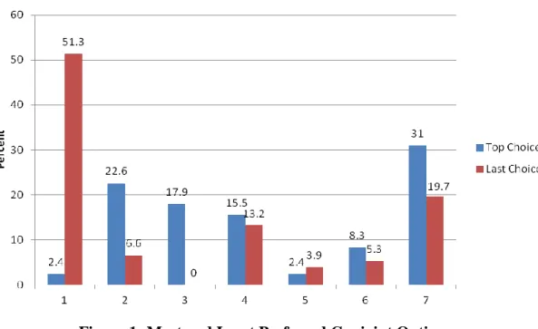
5.3 Results ... 75
5.3.1 Summary Statistics ... 75
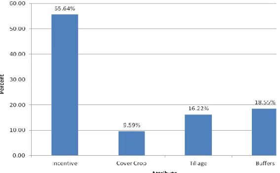
5.3.2 Conjoint Analysis ... 80
5.4 Discussion ... 87
5.4.1 Data Collection Process ... 87
vii
5.4.3 Demographic Analysis ... 91
5.4.4 Conjoint Analysis: Big Picture Conclusions ... 92
5.4.5 BMP Preferences & Part-worth Utilities ... 92
5.4.6 Relative Importance of Attributes ... 94
5.4.7 WTA Incentive Levels ... 94
5.4.8 Program Implications... 96 5.4.9 Next Steps ... 97 5.4.10 Conclusion ... 99 CHAPTER 6: ARTICLE 2 ... 100 6.1 Introduction ... 100 6.1.1 Background ... 100 6.1.2 Literature Review ... 102 6.2 Methods... 107 6.3 Results ... 108 6.4 Discussion ... 124 6.4.1 Cost-Share Amounts ... 124
6.4.2 Application Ranking & Contract Approval ... 125
viii
6.4.4 Structural Improvements vs. Management Practices ... 127
6.4.5 Understanding Program Structure ... 128
6.4.6 Summary of Program Areas to Target ... 129
6.4.7 Farmers “Need to Know” EQIP List ... 129
6.4.8 Next Steps ... 130
6.4.9 Conclusion ... 131
ix
LIST OF TABLES
Table 1: Combinations of conservation practices offered in conjoint question... 55
Table 2: Attribute names, levels, and variable types ... 57
Table 3: Frequencies of Weights ... 59
Table 4: Demographic Characteristics of Conjoint Respondents by Survey Group ... 76
Table 5: Demographic Characteristics of Conjoint Respondents (n=85) ... 78
Table 6: Respondents’ Use of Conservation Practices & EQIP (n=85) ... 78
Table 7: Comparison of Survey Respondents with Vermont Farmer Population ... 80
Table 8: WLS Regression Results ... 82
Table 9: Attribute Part-Worths ... 83
Table 10: WTA of Farmers for Implementation of Conservation Practices ... 85
Table 11: Comparison of Mean Cost/Acre for 3 BMPs ... 86
Table 12: Demographic Characteristics of Respondents (n=61) ... 109
Table 13: Comparison of Survey Respondents with Vermont Farmer Population ... 111
Table 14: Respondent opinions about conservation practices and programs ... 113
Table 15: EQIP Participation Statistics by Main Product ... 115
Table 16: Summary of Respondents’ Experiences with EQIP Contracts ... 117
Table 17: Frequency of Non-monetary Benefits & Challenges Received by Respondents ... 119
Table 18: Frequency of Reasons Respondents had Never Applied to EQIP ... 121
x
LIST OF FIGURES
Figure 1: Most and Least Preferred Conjoint Options ... 81 Figure 2: Relative Importance of Attributes in Farmer Decision-Making ... 84 Figure 3: Frequencies of Structural Improvements in Respondents’ EQIP Contracts ... 115 Figure 4: Frequencies of Management Practices in Respondents’ EQIP Contracts ... 116
1
CHAPTER 1: INTRODUCTION 1.1 Background
The environmental degradation and negative externalities imposed on society by US agricultural production systems have been steadily increasing since the end of World War II (UNCTAD, 2013). These impacts include soil erosion, pollution of waterways and groundwater, greenhouse gas emissions, loss of biodiversity, shrinking wildlife habitat, and pesticide and fertilizer run-off and leaching (Grossman, 2011). Current trends in population growth and demand for food continue to fuel the production, and exacerbate the impact, of these externalities (UNCTAD, 2013). Climate change and variability will further compound the effects of these challenges to the long-term sustainability of agricultural systems (Walthall, Hatfield, Backlund, Lengnick, & Marshall, 2013). The need to ensure the resiliency and viability of our farms and food systems is a pressing and increasingly salient issue.
To incentivize farmers to supply more positive environmental externalities and encourage adherence to environmental regulations, in 1996 the USDA established the Environmental Quality Incentives Program (EQIP). This working lands conservation program provides financial assistance to farmers who wish to address natural resource concerns on their farms by making structural improvements or implementing best
management practices (BMPs). The incentives provided include technical assistance and cost-shares of up to 75% of implementation costs. Given that farmers are navigating the cost-price squeeze and are at times unable to prioritize long-term investments that require large upfront investments, EQIP has the potential to play an important role in
2
simultaneously supporting the economic and environmental sustainability of US farms (Natural Resources Conservation Service, 2012).
In order for EQIP to prove effective at the farm-level, the program must deliver regionally appropriate programs, specifically with regard to incentive levels and technical services (Johansson & Cattaneo, 2006; Winsten et al., 2011). Farmers’ willingness-to-accept incentive levels vary with their demographic and geographic characteristics (Claassen, Cattaneo, & Johansson, 2008; Johansson & Cattaneo, 2006). It follows that determining incentive levels that are cost-effective for both farmers and the federal government is challenging, though studies have shown that setting appropriate incentive levels is a key step in designing effective conservation programs and one that needs a continued regional research focus (Claassen et al., 2008; Cooper & Signorello, 2008; Wossink & Swinton, 2007). An examination of incentive levels does not provide a complete picture of on-farm program effectiveness yet few studies have focused on the functioning of other key program areas at the regional level. This project aims to provide that regional focus, first by calculating Vermont farmers WTA for three common best management practices and then by documenting Vermont farmers’ perspectives on the realized effectiveness of EQIP. The research questions for this study are listed below.
1.2 Article 1 Research Questions
1) What is Vermont farmers’ willingness to accept (WTA) for each conservation practice?
3
3) How may the WTA results inform the implementation of cost-share programs in Vermont?
1.3 Article 2 Research Questions
1) How does EQIP support the resiliency and viability of all types of farms in Vermont? 2) Do Vermont farmers encounter challenges or barriers when enrolling and participating in EQIP?
3) What benefits and opportunities does EQIP participation provide to Vermont farmers? 4) Is the realized effectiveness of EQIP in Vermont aligned with the espoused program goals? If not, what changes could be made to improve that alignment?
4
CHAPTER 2: LITERATURE REVIEW 2.1 Environmental Impacts of Agricultural Systems
The environmental degradation and negative externalities imposed on society by US agricultural production systems have been steadily increasing since the end of World War II (UNCTAD, 2013). These impacts include soil erosion, pollution of waterways and groundwater, greenhouse gas emissions, loss of biodiversity, shrinking wildlife habitat, and pesticide and fertilizer run-off and leaching (Grossman, 2011). Current trends in population growth and demand for food continue to fuel the production, and exacerbate the impact, of these externalities (UNCTAD, 2013). Climate change further compounds these challenges; rising temperatures, increasing geographic and temporal variability of precipitation, extended growing seasons, and increasing frequency of extreme weather conditions are significantly impacting agricultural systems in a
multitude of ways (Walthall et al., 2013). The need to ensure the resiliency and viability of our farms and food systems is a pressing and increasingly salient issue.
The following sections outline the impact of agricultural production on two major natural resources- water and soil. This is followed by a brief discussion of the impacts of climate change and variability on agricultural systems and an overview of agriculture in Vermont.
2.1.1 Water & Agriculture
Agricultural systems in the United States significantly impact both water usage and water quality. US agriculture accounts for 80-90% of all water use with 37% of the total is used specifically for irrigating crops (Osteen, Gottlieb, & Vasavada, 2012).
5
Simultaneously, water bodies and groundwater are contaminated by agricultural leacheates, surface run-off, and waste water disposal. Thus there is a need to address both water use efficiency and water quality (Osteen, Gottlieb, & Vasavada, 2012). The former can be addressed by improving water management practices, for example by upgrading irrigation systems. The latter can be addressed by improving water
management practices through avenues, such as extension outreach, and policy changes, such as Vermont’s renewed focus on total maximum daily load standards for phosphorus entering Lake Champlain (Osteen, Gottlieb, & Vasavada, 2012;
http://www.epa.gov/region1/eco/tmdl/lakechamplain.html).
2.1.2 Soil & Agriculture
Soil quality is a reflection of “the capacity of soil to facilitate nutrient cycling, regulate water flow, maintain physical stability, neutralize environmental pollutants, and provide habitat, food, and fiber (Osteen, Gottlieb, & Vasavada, 2012, p.33).” The higher the quality of the soil, the higher the resiliency of the land to environmental disturbances; this greater degree to mitigate the effect of pollutants and flooding equates to fewer negative externalities being imposed on society by farms with poor soil quality (Osteen, Gottlieb, & Vasavada, 2012). Additionally, in 2007 approximately 27% of the cropland in the US was classified as highly erodible (Osteen, Gottlieb, & Vasavada, 2012). Good soil quality and management decrease the rate of erosion and thus the amount of
6
2.1.3 Climate Change & Agriculture
Climate change has had, and will continue to have, a multitude of both beneficial and detrimental impacts on US agricultural systems (UNCTAD, 2013; Walthall et al., 2013). Crop growth is a function of temperature, precipitation, water availability, carbon dioxide levels, and solar radiation. Increasing temperatures and carbon dioxide levels will allow for faster, more vigorous plant growth however weed pressure and the plants’ demand for water will simultaneously intensify (Walthall et al., 2013). Livestock health will likely be negatively impacted even as the production of their feed is positively affected (Walthall et al., 2013). The higher temperatures, resulting in more frost-free days, will likely disrupt pollination, lead to the need to shift away from crops or cultivars with certain temperature requirements, and cause changes in the
regional composition of pest, pathogen, and weed species populations (Walthall et al., 2013). As precipitation increases and becomes more variable, erosion and run-off rates may increase and become more severe, especially on farms using conventional tillage and leaving ground fallow (Walthall et al., 2013). As droughts and high temperatures become more common, water shortages may cause costs of production to increase as irrigation becomes more expensive (Walthall et al., 2013). All told, the net effects of climate change on agricultural systems are, and will remain, highly heterogenous and dependent on the many spatial, temporal, and biophysical variables of the agricultural system being examined.
7
2.1.4 Brief Overview of Vermont Agriculture
Vermont has 7,338 farms on 1,251,713 acres of cropland, woodland, and
pastureland (2012 Census of Agriculture). The mean farm size is 171 acres (2012 Census of Agriculture). The hilly, rocky terrain is composed of a wide variety of soil types suitable for growing a variety of crops, although pastures and hay are predominant. Summer temperatures typically range from 51-82°F while winter temperatures tend to remain between 0-30°F (www.agclassroom.org/vt). Dairy production accounts for 72% of the value of Vermont’s agricultural products (www.agclassroom.org/vt). Vermont’s climate, terrain, and composition of its agricultural economy are similar to that of other Northeastern states but unlike that of the rest of the country. This directly influences the scale and product type of Vermont farms and the selection of management practices employed by Vermont farmers; each is different from that of farmers in other geographic location. This fact will be especially relevant in the ensuing discussion of incentivizing the adoption of best management practices by Vermont farmers.
2.2 Resiliency in Agricultural Systems
Farmers need access to land and water in order to grow and sell their products and remain in business. The way in which each farmer chooses to manage their natural resource base is influenced by many factors including the farmers’ educational
background, public policies, and market forces (Osteen, Gottlieb, & Vasavada, 2012). In addition, farmers need to be prepared to adapt to a multitude of stimuli generated by climatic variability in the short run and climate change in the long run (Bryant et al.,
8
2000). Decisions made in all arenas and at all temporal scales will influence the viability of their operations (Smit, Burton, Klein, Richard, & Wandel, 2000). It is the hope that different temporal adaptations will be iterative and that short-term management strategies to deal with current environmental and climatic conditions will also improve farmers’ ability to adapt in the long-term (Howden et al., 2007; Adger et al., 2005).
Resiliency is defined as “the degree to which a system rebounds, recoups, or recovers from a stimulus (Smit et al., 2000, p.238)." These stimuli may include changes to the physical, political, social, or economic farm environment (Smit & Skinner, 2002). Research has shown that farmers’ adaptive responses to these changes tend to involve a modification of an existing agronomic practice they or their neighbors already employ (Smit & Skinner, 2002). Farmer demographics, market supply chains, the degree of system exposure and vulnerability, whether or not the change was anticipated, and the economic implications of the chosen strategy all influence what type and scale of
adaptation is chosen and whether the adaptation is spontaneous or planned (Bryant et al., 2000; Smit & Wandel, 2006; Smit et al., 2000). Adaptive responses can be reactive or proactive and occur on many different scales ranging from individual farmer’s’ actions to government interventions (Bryant et al., 2000; Smit & Wandel, 2006; Smit et al., 2000).
9
2.3 Best Management Practices
This research focuses on farmer adoption of best management practices (BMPs), which is one option available to farmers who wish to adapt their systems to address on-farm natural resource concerns. The USDA defines BMPs as “established soil
conservation practices that also provide water quality benefits (Gold, 2007).” Examples of common BMPs include cover cropping, stripcropping, and appropriate fertilizer application rates (Gold, 2007). Implementation of BMPs allows farmers to improve the overall resiliency of their land while simultaneously generating economic returns (Howden et al., 2007). For example, a farmer’s decision to adopt conservation tillage techniques leads to less erosion, reduced compaction, and improved moisture retention of their land; this reduces equipment, fuel, and labor costs while improving the long-term health of their soil and the resiliency of their land (Wall & Smit, 2005).
The USDA and other agricultural technical service providers are increasingly emphasizing the need for farmers to adopt BMPs to address environmental health concerns, ensure the long-term sustainability of their operations, and to use as an adaptation strategy for coping with climate change (Walthall et al., 2013). Bradshaw, Dolan and Smit (2004) emphasize the importance of regional field testing of best
management practices to ensure the strategies are a suitable match for the type and size of farm operations for which they are being recommended. This research is part of an on-going effort in Vermont to examine what types of farms are using which best
management practices, the outcomes of using those practices, and what governs farmers’ decisions to employ those adaptive strategies. The overall trends in the literature
10
examining farmer adoption of BMPs are discussed below in order to set the stage for this specific research project.
2.4 Farmer Adoption of Best Management Practices
The decision-making processes surrounding farmers’ management decisions are embedded in their social, biophysical, institutional, and economic environments (Wall & Smit, 2005). One way to understand farmers’ patterns of adoption for agricultural innovations such as BMPs is through diffusion models. The best known is Everett Rogers’ 1962 theory which outlines how innovations spread through society (Rogers, 2003). Central to Rogers’ theory are the key categories of adopters which are separated according to speed of adoption into innovators, early adopters, the early majority, the late majority, and laggards (Rogers, 2003). Four characteristics of innovations- complexity, compatibility, trialability, and observability- are also integral to Roger’s (2003)
explanation. Linking the characteristics of an innovation with the traits and avenues of communication used by adopters explains why certain innovations are adopted at a rapid rate, while others are not adopted or spread more slowly (Rogers, 2003).
Rogers’ diffusion theory is the most widely utilized, however in 1981 Lawrence Brown published an alternative theory that has also been frequently applied. Brown held that the paths of innovation diffusion are dependent on the entity that supplies the
innovation as that entity is in the position to regulate who the innovators and early adopters will be, thereby affecting the entire cycle of the diffusion process (Brown, 1981). While it is important to recognize Brown’s contribution to diffusion theory, it is
11
not generally employed by diffusion scholars examining the spread of agricultural adaptation strategies. Due to their tacit nature, adaptive agricultural innovations do not fit well into Brown’s supply management framework. In addition, adoption decisions about agricultural innovations tend to occur at the individual or household level instead of at the firm or distributor level (Feder & Umali, 1993). Therefore the majority of the literature focused on the diffusion of adaptations amongst farmers examines patterns by applying Rogers’ model.
Many studies have examined the demographic and farm characteristics as well as the motivations of farmers who adopt best management practices. Although results vary with the methods employed, many trends of significant demographic variables and character traits exist in the literature. Farmers who have obtained higher levels of education, possess a higher degree of environmental awareness, and have more
knowledge about the impacts of agricultural practices on the environmentare more likely to implement BMPs than their peers (Prokopy, Floress, Klotthor-Weinkauf, & Baumgart-Getz, 2008; Ryan, Erickson, & De Young, 2003; Saltiel, Bauder, & Palakovich, 1994; Stock, 2007). BMPs are also more likely to be adopted by farmers whose peer networks support and promote the practices (Carolan, 2005). This indicates that innovations which mesh well with farmers’ perceptions of self, socioeconomic status, and background and which preserve their primary source of social capital have a greater likelihood of being adopted (Carolan, 2005; Risbey, Kandlikar, Dowlatabadi, & Graetz, 1999). In addition, farmers with diversified operations and those who derive intangible value from the health of their land are more likely to implement BMPs (Prokopy et al., 2008; Ryan et al., 2003;
12
Wall & Smit, 2005). This is significant because sustainable agricultural practitioners by nature tend to be reflexive, rather than prescriptive, growers, a valuable quality given the unpredictability of the farming profession (Stock, 2007).
Due to the usefulness of Rogers’ diffusion theory in linking the spread of innovations to adopter characteristics, researchers have most frequently studied the demographic characteristics of farmer adopters. However, a variety of farm structure, agroclimatic, and BMP characteristics have also been identified as significant variables influencing the adoption of BMPs by farmers (Camboni & Napier, 1993; Ryan et al., 2003; Saltiel et al., 1994; Webb, 2004). Both the overall farm structure and the specific enterprises the farmer is engaged in strongly influence the ease in which a BMP is adopted and integrated into the management system (Camboni & Napier, 1993; Saltiel et al., 1994). The BMPs which are most frequently adopted are generally low in
complexity, highly compatible with the existing farm system, high in trialability, and high in observability (Webb, 2004). Farm scale is positively correlated to adoption, with larger farms more likely to adopt BMPs (Feder & Umali, 1993; Prokopy et al., 2008; Ryan et al., 2003). As scale increases, income level, capital, and hired labor also tend to increase; it follows that those three variables are usually positively correlated to BMP adoption as well (Prokopy et al., 2008; Ryan et al., 2003). The agroclimatic environment of the farm can also affect the adoption of BMPs and it follows that the relative influence of all of the variables identified above, as well as types of BMPs adopted, will vary by region (Feder & Umali, 1993; Webb, 2004). The failure of Knowler and Bradshaw (2007) to find any significant variables at the global level that could universally describe
13
adoption patterns or the motivations of farmers who adopt BMPs further suggests the need to use an appropriate scale when undertaking adoption research. This point will be important later in examining conservation program design and the need for regional specificity in order to maximize its effectiveness (Bradshaw et al., 2004; Knowler & Bradshaw, 2007).
2.5 Economic influences on decision-making
The influence of demographic, farm, agroclimatic, and BMP characteristics on farmers’ decisions to adopt BMPs should not be discounted yet the economics behind the choice to adopt influences decision-making more than any other factor. The practice needs to be profitable and the perceived risk associated with implementing the practice low enough in order for widespread adoption to occur (Camboni & Napier, 1993; Marra, Pannell, & Ghadim, 2003; Saltiel et al., 1994; Webb, 2004). Farmers implementing BMPs tend to create positive externalities in the form of ecosystem services; if the costs of implementation are greater than the private benefits produced, farmers are privately funding public goods (Kroeger & Casey, 2007; Lichtenberg & Smith-Ramirez, 2011). As public goods are non-rival and non-excludable, if farmers do not perceive enough of a threat to their farm systems to warrant adoption they will be better off financially not implementing a BMP regardless of any existing environmental concerns; this lack of proactive adoption can result in the underproduction of ecosystem services and is detrimental to both the farm operation and society (Cary & Wilkinson, 1997; Kroeger & Casey, 2007; E. Lichtenberg & Smith-Ramirez, 2011).
14
At the most basic level, a practice is profitable if the costs associated with implementation are less than the resulting benefits (Mendelsohn, 2000). Pannell (1999) takes this definition one step further and states that a practice should produce benefits that outweigh both the direct costs and opportunity costs of adopting that practice. Weighing the opportunity cost in the implementation decision can be especially important in farm systems where the value of time is at a premium. Time spent implementing a BMP may mean less time for other farm tasks and possibly less economic profit overall in the short term; this line of reasoning may be why many farmers perceive BMPs to be an “income drag” on their bottom line, regardless of whether that perception has any grounding in reality (Valentin, Bernardo, & Kastens, 2004). The difficulty in altering this perception lies in the fact that, though the costs are accrued in the short-term, the benefits of
implementing BMPs may only be tangible in the medium or long term (Bradshaw et al., 2004; Pannell, 1999; Risbey et al., 1999). Crop yields are the most visible short-term performance measure of BMP adoption; however, just as yield is not always an accurate indicator of farm profitability, that measure does not always serve as a reliable indicator of long-term success for BMPs (Risbey et al., 1999). If the BMP is being implemented by a farmer who is examining the economic, environmental, and social sustainability of their farm at all temporal scales, measures of successful BMP adoption should examine the level of resiliency and long-term sustainability of the agricultural system (Risbey et al., 1999).
The other economic factor complicating farmers’ BMP implementation decisions is the influence of the perceived risks associated with adoption. The farmer needs to
15
perceive that the risk to the viability of their business, either at the environmental or farm level, outweighs the risk of implementing a new practice (Cary & Wilkinson, 1997). This can become a significant barrier to adoption as perceived profitability tends to trump environmental concerns in farmers’ decisions (Cary & Wilkinson, 1997). If enough of a risk is perceived, the farmer then examines the realized and intangible costs, benefits, and potential effects of implementation on their operation (Marra et al., 2003). As discussed above, assessing this situation may prove challenging if it is unclear when the benefits and costs will actually accrue. This can leave the decision-making process largely dependent on the type and amount of information available about the practice and the degree of risk-averseness of the farmer (Marra et al., 2003; Mendelsohn, 2000; Pannell, 1999). As the need for adoption increases, farmers may also want to examine the possibility of joint BMP adoption in order to reduce the level of risk assumed by each individual implementing a particular practice (Mendelsohn, 2000). By taking collective action, it is possible to form a network of knowledge and technology sharing and
implement regional solutions that benefit many farmers (Mendelsohn, 2000).
2.6 Incentives for BMP Implementation
If the benefits of either individual or joint adoption do not outweigh the cost of implementation and affect the rate of BMP adoption, government intervention may be necessary. Federal incentivized conservation programs assist farmers in overcoming the economic barriers to BMP adoption, subsequently improving the long term profitability and resiliency of their operations (Bryant et al., 2000). These programs serve to
16
counteract the underproduction of public goods and encourage the prosperity of
agricultural systems without compromising the health of the environment (Lichtenberg & Smith-Ramirez, 2011; Smith, 2006).
In order to achieve these goals, conservation programs address the two main economic barriers to farmer adoption of BMPs- profitability and the perceived risks of implementation (Camboni & Napier, 1993; Marra et al., 2003; Saltiel et al., 1994; Webb, 2004). Indeed, it has been shown that farmers’ supply of conservation practices responds to changes in incentive payments. For example, Kurkalova et al. (2006) demonstrated that acreage in conservation tillage supplied increases with the level of subsidy offered per acre. Many other conservation practices, such as strip cropping, contour farming, terracing, and cover cropping have been found to have a positive elastic response to a 1% change in the cost of the practice to the farmer (Lichtenberg, 2004). This elasticity increased when complimentary combinations of practices were analyzed; incentivizing combinations proved to be cheaper, and yield more environmental benefits, than practices implemented in isolation (Lichtenberg, 2004). Farmers are also more likely to supply an ecosystem service when it is produced jointly with a marketable farm product (Wossink & Swinton, 2007). This willingness of farmers to supply ecosystem services when the practice is complementary, or even enhances, the rest of the business is further evidence that economics tends to trump social and environmental considerations in farmers’ BMP adoption decisions.
Incentive payments compensate farmers for a portion of the direct implementation costs and include a risk premium to offset the uncertainty associated with adoption
17
(Cooper & Signorello, 2008; Kurkalova et al., 2006). Required components of incentive payments will vary in quantity from farmer to farmer as will the magnitude of the weight given to risk aversion, direct costs, and opportunity costs in their decision-making process; at times an individual’s risk-aversion may be so strong that it prohibits adoption even when expected profits with BMP implementation are higher than those generated with the current management system (Kurkalova et al., 2006; Wossink & Swinton, 2007). Thus the challenge for formulating incentive levels is in finding a value high enough to increase the overall rate of adoption and low enough to maintain the cost-effectiveness of the conservation program (Feder & Umali, 1993). Few studies have calculated
percentages that can be used to formulate appropriate incentive levels (see Cooper & Signorello, 2008 and Kurkalova et al., 2006 for examples). Determining accurate figures for farmers’ willingness-to-accept (WTA) for implementing conservation practices is a key step in designing effective public policy and one that needs a continued regional research focus (Claassen et al., 2008; Cooper & Signorello, 2008; Wossink & Swinton, 2007).
2.7 Environmental Quality Incentives Program
In response to the need to address environmental health concerns and correct the temporal and distributional inequities affecting farmer adoption behavior in the failing market for ecosystem services, in 1996 the federal government authorized the
Environmental Quality Incentives Program (EQIP). The overarching goals of EQIP are to support the co-production of agricultural products and environmental quality and to
18
assist farmers in complying with the minimum standards of environmental regulations. It is important to note that EQIP is not the only USDA conservation program. The others include the Agricultural Management Assistance Program (AMA) and the Conservation Stewardship Program (CSP). This project focuses on EQIP because it has the highest rate of participation, funds the largest scope of projects, and may be utilized by a diversity of farm types.
Through EQIP, incentives are provided in the form of cost-sharing and technical assistance to farmers who wish to make structural improvements or implement BMPs. Natural resource concerns, such as water quality, soil erosion, air quality, energy
conservation, and preservation of biodiversity, must be directly addressed by the project in order to qualify for funding. EQIP contracts may be one to ten years in duration and cover up to 75% of incurred expenses with cost-share funds. Payments are made to farmers upon completion of each project in their contracts.
EQIP needs to be effective at the farm-level while producing the results the government desires within the constraints of the allocated budget. Cost effectiveness at the federal level is tracked not only through total expenditures per acre but also by environmental benefit per dollar spent but the realized effectiveness of the program is dependent on far more than these two metrics. Three specific areas- funding, contract approval, and incentive payments- influencing to the cost-effectiveness of EQIP at the farm and federal levels are addressed below. Following that, the USDA’s method of examining project results and its voluntary approach to conservation programs are discussed. This review of EQIP will conclude by identifying research needs.
19
2.7.1 EQIP: Funding
USDA incentivized conservation programs are federally funded but implemented by state NRCS offices. Both NRCS and the conservation programs it administers are entrenched in the mandatory spending category in the USDA budget while funding for conservation technical assistance, a key part of program implementation, is categorized as discretionary funding (USDA, 2013). Each year conservation projects compose about 7% ($1.4 billion in 2012) of the total USDA budget (www.nrcs.usda.gov). In fiscal year 2011, that included 38,352 EQIP contracts approved or completed for a total of
$864,860,399 obligated for conservation projects on 13,162,935 acres across the United States (www.nrcs.usda.gov). Vermont had 373 active or completed EQIP contracts on 42,589 acres funded with $9.48 million dollars of federal incentive money
(www.nrcs.usda.gov). Despite increasing levels of funding since the program began in 1996, funding gaps have become a regular occurrence in recent years which in turn has affected program delivery (Eubanks, 2009). In addition, though EQIP is projected to be minimally affected, the 2014 Farm Bill reduces aggregate spending on conservation programs by $4 billion over the next ten years. These funding gaps and reductions,
coupled with the federal government’s goal of maximizing environmental benefit per dollar expended, has contributed to the trend of NRCS targeting large farms with
conservation money; the economy of scale rule dictates that contracts for large farms are more efficient at reducing environmental harm and have lower administrative transaction costs per acre than those for small farms (Eubanks, 2009). Annual funding is one way to
20
measure program health yet it is a one-dimensional metric and other components are needed add complexity to the examination of EQIP effectiveness.
2.7.2 EQIP: Contract Approval Process
When farmers submit EQIP contracts, NRCS staff evaluate and approve
program applications according to the environmental and resource concerns prioritized by the state as targets for program initiatives. A weighted environmental index is created and utilized to rank farmers’ EQIP applications and determine which contracts will maximize environmental benefit per dollar expended. It is important to note that the environmental priorities the incentives will address are determined by government officials and state conservation service employees, not farmers (Johansson & Cattaneo, 2006; Smith, 2006). This is significant because it has been demonstrated that the form of these environmental indices affects the function and outcomes of EQIP; the weights assigned to environmental components represent trade-offs between, and government valuation of, various components of the state’s natural resource base (Johansson & Cattaneo, 2006). It follows that appropriate regional indices would help ensure enrollment of farmers who are implementing practices that address the most pertinent environmental concerns in the area (Johansson & Cattaneo, 2006). Regional policies also provide specific incentives leading to targeted results instead of approving cost-shares for practices that are more effective at solving resource concerns in other regions of the country (Smith, 2006). In addition, regional indices may also benefit farmers by funding conservation practices that fit their farm systems, leading to the joint production of
21
ecosystem services and marketable products while simultaneously increase the aggregate adoption rate of BMPs (Wossink & Swinton, 2007).
2.7.3 EQIP: Cost-share Payments
After an application is approved, a contract is offered to the farmer, outlining the cost-share and technical assistance NRCS can offer for the practices or structures the farmer wishes to implement. Economically, this is NRCS’ demand curve for particular practices, or, stated otherwise, its willingness-to-pay (WTP) as a consumer of
conservation services, and it varies according to regional environmental priorities (Kroeger & Casey, 2007). Unlike a traditional supply and demand model where the producers set the prices, in this case the farmers are price-takers and NRCS is both the consumer and the price-setter. Whether or not the farmer accepts the offer made by NRCS is largely dependent on their individual WTA. Plotting farmers’ WTA generates a supply curve that can represent either acres managed using BMPs or the quantity of agri-environmental benefits produced as a result of the BMPs implemented (Kurkalova et al., 2006; Smith, 2006; Swinton, Lupi, Robertson, & Hamilton, 2007; Wossink & Swinton, 2007). It follows that the equilibrium point of these supply and demand curves
represents the point where farmers’ aggregate WTA and the government’s WTP are equal, which would be an indication that EQIP is functioning effectively at both the farm and federal levels (Swinton et al., 2007).
As noted above, more research is needed to determine mean regional levels of WTA as demographic, geographic, farm characteristics, and degree of risk averseness directly affect the minimum support a farmer requires (Claassen et al., 2008; Wossink &
22
Swinton, 2007). If incentive payments are too low, the enrollment process might not be worth the farmers’ time and low participation rates might affect the long-term viability of conservation programs. However, the cost effectiveness of the program, number of contracts funded, and the net environmental benefit generated by the program will decrease if the government offers cost-share amounts in significant excess of farmers’ WTA (Claassen et al., 2008; Yano & Blandford, 2009). The latter situation has
previously occurred in the Conservation Reserve Program; Claassen et al. (2008) found 10-40% of payments received were above the minimum amount farmers were willing to accept.
No simple solution appears to exist that would allow a straightforward reduction in the difference, for either excess or insufficient funds, between cost-shares offered and farmers’ WTA. This is because there is inherently information asymmetry present in the relationship between farmers and NRCS staff (Cattaneo, 2003; Claassen et al., 2008; Yano & Blandford, 2009). Farmers can estimate their WTA based on their true costs, potential benefits, and expected risk. NRCS has rough estimates of costs and the awareness that a premium to offset risk should be included in the cost share (Cattaneo, 2003). Not only does this mean that NRCS’ price schedule for structures and BMPs does not work for all farmers but it creates the potential for adverse selection (Cattaneo, 2003). For example, it has been found that cost-share incentives were actually functioning like income transfers when granted to farmers for whom adoption of a BMP would have been profitable or preferable even without incentive assistance (Horan & Claassen, 2007; Kurkalova et al., 2006; Lichtenberg & Smith-Ramirez, 2011). Thus, while there is
23
evidence that cost-share programs like EQIP do in fact increase the probability that farmers will implement conservation practices, there is clearly work to be done to ensure that incentive payments are cost-effective for both farmers and taxpayers (Lichtenberg & Smith-Ramirez, 2011).
2.7.4 EQIP: Voluntary Approach to Conservation
Farmers who choose to enroll in EQIP do so voluntarily. This approach is intended to leave the power to make management decisions with farmers, potentially increasing the program participation rate and reducing government expenditures for transaction and enforcement costs compared to mandatory standards (Horne, 2006; Khanna, 2001; Lal, 2004). However, it has been called into question as to whether farmers have enough flexibility with their time and resources to make a voluntary approach to conservation effective in the current US agricultural systems (Eubanks, 2011). Effectiveness could potentially be improved if programs focused more on outcomes rather than outputs (Winsten et al., 2011). The current system provides incentives for farmers to implement projects and practices; alternatively, result-driven incentives could be provided for farmers to achieve specific environmental outcomes (Winsten et al., 2011). That change would entail overhauling EQIP to more closely resemble the structure of the CSP. Such an evaluation is beyond the scope of this research, however it appears that this could provide farmers volunteering to enroll in EQIP a higher level of motivation to meet and exceed the minimum environmental standards while simultaneously maximizing the short and long-term benefits of the program at the farm-level (Winsten et al., 2011).
24
2.7.5 EQIP: Contract Outcomes
In order to determine if the program components discussed above are generating the expected results and to improve the effectiveness of EQIP, completed contracts need to be monitored in order to determine what outcomes the program generates. Both the evaluation of environmental benefit, due largely to a lack of baseline data, and issues with contract monitoring are persistent problems for NRCS staff (Claassen et al., 2008). Performance measures currently used to evaluate EQIP include the number of nutrient management plans developed and acres of crop, grazing, and forested land managed with conservation plans (www.nrcs.usda.gov). Quantitative environmental effect values drawn from the literature are then assigned to all components of these performance measures in USDA cost-benefit program evaluations. A more direct effort to identify and measure program outputs and outcomes was launched in 2005 when the Conservation Effects Assessment Program was established (Duriancik et al., 2008; Stubbs, 2010). However, results from this multi-organizational endeavor have been limited in scope and it remains unclear as to whether that data will establish causal linkages between
implemented practices and environmental improvements at regional or farm scales
(Duriancik et al., 2008). Smith (2006) suggests that the reason for these challenges is that funded projects attempt to improve many different environmental problems
simultaneously; this presents practical measurement issues, leading to difficulties producing direct evidence that cost-share funds are generating the anticipated benefits.
It is also unclear whether projects are always carried out as contracted. This lack of clarity arises due to limited staff resources or incentives becoming perverse. If the
25
staff time is limited, project monitoring may not occur with adequate frequency. These situations necessitate federal and state NRCS staff take farmers at their word that contracts are being fulfilled (Cattaneo, 2003; Yano & Blandford, 2009). Limited staff time may also correlate to reasons behind why certain contract decisions do not seem to reflect the stated goals of EQIP. For example, in a survey of over 400 Maryland farms, there was no correlation between the applicants’ proximity to water or specific
environmental issues and the receipt of cost-share funds, despite Maryland’s emphasis on cleaning up Chesapeake Bay (Lichtenberg & Smith-Ramirez, 2011). Yet, it appears that there is a new commitment to funding monitoring projects; although no monitoring and evaluation contracts were funded from 1996-2008, starting in 2012, $482,144 has been allocated for 69 monitoring projects, 11 of which had been completed as of May 2013 (Natural Resources Conservation Service, 2013).
The second reason contracts may not always generate the intended program outcome is that, in some instances, incentivized contracts create situations of perverse decision-making. Incentives have been found to reduce the amount of farm acreage covered by vegetation and to increase production occurring on marginal land
(Lichtenberg & Smith-Ramirez, 2011). Large farms, especially operations for which increased acreage means increasing returns to scale, may cause more environmental damage by increasing production on marginal land not previously included in their rotation (Eubanks, 2011; Yano & Blandford, 2009). It is not evident in the literature whether this is a common occurrence. Instituting a compliance reward system to counter any tendencies towards this form of systemic noncompliance may be necessary in some
26
areas and could be achieved by restructuring payments to encourage the generation of measurable performance-based program outcomes (Yano & Blandford, 2009).
2.7.5 EQIP: Research Needs
All of the program components discussed above frame various aspects of the ways farmers interface with EQIP. A complete examination of program effectiveness should also objectively examine the experiences of farmers participating in the program and the impact of their participation on their businesses. A 2010 survey elicited
significant differences between the viewpoints of academics, government officials, NGO employees, and farmers as to whether EQIP is effectively fostering the implementation of sustainable agricultural practices (Bailey & Merrigan, 2010). Opinions of each group varied by practice, but overall only 73% of practices funded by EQIP were judged to be advancing environmental sustainability (Bailey & Merrigan, 2010). The reasons for this discrepancy with the espoused theory of the program are not addressed by the survey authors but may be embedded in the research of others. The difference could be rooted in farmers, academics, government officials, and NGO employees each subscribing to a different definition of sustainability. Farmers’ perceptions of program accessibility may also have been affected by the fact that both average contract size and the number of unfunded applications have increased since program inception which could have decreased the perceived on-farm economic sustainability of EQIP (Stubbs, 2010). Additionally, in the first five-years of the program there was a 17% farmer withdrawal rate of approved contracts and practices. This potentially indicates that the contracts NRCS staff felt were encouraging sustainability either did not parallel farmers’ definition
27
or fit their management systems (Cattaneo, 2003). To fully evaluate the effectiveness of EQIP, the shortage of research examining the program at the farm-level must be
addressed.
As discussed above, this EQIP research should be conducted regionally in order to determine appropriate incentive levels and determine how effective the program is at the farm level. This research aims to provide that regional focus by examining three BMPs- conservation tillage, cover cropping, and conservation buffer strips- eligible for cost-sharing through EQIP. Though these are three among many different structural and conservation practices eligible for funding, after consultation with extension staff these three practices were selected based on applicability to a diversity of farm types in Vermont and the potential of each practice to help farmers address natural resources issues on their land while generating an indirect economic return. In the following sections, each practice is described and the benefits, costs, and ways each strategy improves the health of the environment while increasing the resilience of agricultural systems are identified.
2.8 Cover Crops
Cover crops are grasses, legumes, or forbs planted by farmers in order to protect and improve the soil (NRCS, 2008). A diversity of temporal, spatial, and varietal options are available to farmers determining the cover cropping approach that best fits their farm system (Sarrantonio & Gallandt, 2003; Snapp et al., 2005). Examples of cover crops suitable to the climate in the Northeastern United States and commonly used by Vermont
28
farmers include winter rye, oats, peas, hairy vetch, and buckwheat (SARE, 2007; Sarrantonio & Gallandt, 2003). Farmers choose among these and other types of cover crops and determine whether to interseed, cover fallow ground in-season, or seed down a cover for the winter (SARE, 2007; Sarrantonio & Gallandt, 2003). Ultimately, varietal traits must be matched with the farmer’s management goals, field availability, financial resources, and mechanical capabilities (SARE, 2007; Snapp et al., 2005). An in-depth discussion of cover cropping options is beyond the scope of this project; the focus will be on the benefits and costs of cover cropping and the role of the practice in increasing farms’ resiliency.
The benefits of cover cropping can be divided into two main categories- agri-environmental and economic- and can be reaped by both the farmer and the general public (Sarrantonio & Gallandt, 2003; Snapp et al., 2005). Agri-environmental and economic benefits tend to form a positive feedback loop; the money invested in planting cover crops is generally repaid in agronomic and nonmonetary benefits in the long-term (Snapp et al., 2005). This interconnectedness generates systemic benefits which increase the ability of a farm to withstand variable changes in the environment (Snapp et al., 2005).
Many agri-environmental benefits of cover cropping are generated as the practice both conserves and improves the physical structure of the soil. The roots of cover crops hold soil in place while the above-ground plant biomass protects the soil from the impact of precipitation, significantly reducing erosion due to wind, water, and run-off (Frye & Blevins, 1989; Hartwig & Ammon, 2002; SARE, 2007; Sarrantonio & Gallandt, 2003).
29
Cover crops aid in increasing soil organic matter and improving soil structure which in turn improves infiltration capacity, conserves moisture, and reduces nutrient leaching (Frye & Blevins, 1989; Hartwig & Ammon, 2002; SARE, 2007; Sarrantonio & Gallandt, 2003). Leguminous cover crops not only uptake leaching nutrients but also capture and fix available nitrogen (SARE, 2007; Snapp et al., 2005). In cover cropped areas, Wyland et al. (1996) demonstrated a 65-70% reduction in nitrate leaching, an increased
availability of nitrogen to the cash crop, and higher broccoli yields compared to the winter fallow plots. Similarly, Frye and Blevins (1989) found that using a legume cover crop with minimal tillage increased corn yields compared to systems involving a winter fallow period and use of synthetic fertilizers. Other agri-environmental benefits of cover cropping may include weed suppression and decreased incidence of pests and disease (Frye & Blevins, 1989; Hartwig & Ammon, 2002; SARE, 2007; Sarrantonio & Gallandt, 2003; Snapp et al., 2005).
This multitude of agri-environmental benefits generated by cover cropping leads to the increased sustainability of both the farmland and the surrounding environment (Sarrantonio & Gallandt, 2003). Reducing soil erosion and nutrient run-off improves water quality and soil health throughout watersheds (Hartwig & Ammon, 2002;
Sarrantonio & Gallandt, 2003). Improving nitrogen availability, soil tilth, and soil organic matter may lead to a decreased need for application of synthetic fertilizers, weed
suppression may reduce the need for herbicides, and pest and disease control can potentially mean less use of pesticides and fungicides (SARE, 2007; Sarrantonio & Gallandt, 2003). As a result, farmers receive a direct economic benefit while
30
simultaneously improving the health of the surrounding environment and increasing the resiliency of their land.
Although planting cover crops has been shown to be beneficial to agricultural systems, management decisions necessitate weighing the costs against the benefits. Specific direct costs accrued in most cover cropping systems include: land preparation, seed and seeding, a method of killing the cover crop (i.e mowing, herbicides, tilling) and incorporation (Tourte, Buchanan, Klonsky, & Mountjoy, 2003a). These categories are generalizable to many farm types and sizes yet realized costs are highly variable among farms; for example, a small vegetable farm may find cover cropping much more
expensive on a per acre basis than a large dairy farm (H. Darby, personnel
communication, November 9, 2012). Estimates range from $45 to $65 per acre for a large dairy farm and up to $70 per acre for a farm performing primary tillage before seeding (Tourte et al., 2003; H. Darby, personnel communication, November 2, 2012). Reflecting this fact, the SARE publication Managing Cover Crops Profitably (2007) does not provide a specific budget for cover cropping but instead provides information to guide farmers as they explore cover cropping options. Wyland et al. (1996) also report general budget guidelines, specifically that the cost of winter cover cropping in their system was 5% of the cost of growing the cash crop that followed the cover and that 14% of the total cost of the cover would have been incurred in routine maintenance of a fallow field. It is thus important for farmers to consider their available resources, farm size, and management goals as they create cover cropping expense budgets tailored to their
31
Despite the variation between farms, the direct costs of cover crop establishment are fairly straightforward to compile compared to the indirect costs, opportunity costs, and associated risks of implementation; these are also important factors in farm
management decisions and provide some insight into why providing incentive payments for cover cropping can be helpful in promoting the adoption of the practice (Sarrantonio & Gallandt, 2003; Snapp et al., 2005). Indirect costs of cover cropping may include interfering with planting schedules, issues with cover crop management and
incorporation, and resource competition between the cover and cash crop (Hartwig & Ammon, 2002; Sarrantonio & Gallandt, 2003; Wyland et al., 1996). The opportunity cost of cover cropping may be significant if the decision is made to plant the cover at a time when the field could be used for a cash crop (Sarrantonio & Gallandt, 2003). Farmers, especially those lacking experience with this BMP, must weigh the risk of a cover crop interfering with their management plans and expected profits against the potential benefits of planting; here again the balance of short-term profits with long-term
sustainability is at the root of the adoption decision (Sarrantonio & Gallandt, 2003). If the direct costs to the farmer are greater than the perceived private benefits, cost-shares are needed to incentivize farmers to look beyond the short-term constraints and adopt this BMP (Snapp et al., 2005). Cover cropping is one of many BMPs that qualify for cost-sharing under EQIP.
32
2.9 Conservation Tillage
Conservation tillage is a best management practice that leaves at least 30% of crop or cover crop residue remaining on the surface of the soil when the field is prepared for planting (Gold, 2007). No till and zone tillage systems are the two types of
conservation tillage that will be discussed here. The practices and specific costs associated with each vary and will be addressed separately but the ways each approach helps farmers adapt to climate change is similar and will be discussed together.
Conservation tillage involves preparing land for planting without the use of conventional tillage implements such as plows or disks. Many farmers choose to kill the cover crop using an herbicide but this can also be achieved by crushing and flattening the cover crop using a roller-crimper, cultipacker, undercutter, or mower. In a no-till
operation, a specialized seeder or transplanter is then used to rip a narrow strip through the cover crop into which the seeds or transplants are dropped (Rodale Institute, 2011). In contrast, zone tillage disturbs slightly more of the total ground surface (about 1/3) as 6-10” wide strips are tilled into the cover crop mat. Strip depth is typically 4-6” although deep zone tillage rips below the 6” plow pan and may penetrate as deep as 22”. Crops are then seeded or transplanted into the tilled strips (Idowu, Rangarajan, van Es, & Schindelbeck, n.d.; Rangarajan, 2011). Zone tillage has the potential for farms using low-input and organic practices to get the combined benefits of no till and conventional tillage practices (Idowu et al., n.d.; Rangarajan, 2011). Both systems of conservation tillage provide many agri-environmental and economic benefits to agricultural operations.
33
Conservation tillage generates agri-environmental benefits by fostering soil conservation and improving the physical structure of the soil. Reduced tillage activity and the plant residue left on the surface significantly reduce erosion from both water and wind (Rodale Institute, 2011; Uri, 2001). Soil structure improvements are evident in the increased microbial activity and higher soil organic matter content; this means higher quality soil tilth and aggregation which allows for improved drainage and nutrient retention (Rodale Institute, 2011; Uri, 2001). In addition, the cover crop residue left on the surface of the soil retains moisture, regulates soil temperature, and suppresses weeds (Rodale Institute, 2011; N. D. Uri, 2000). These benefits improve the overall resiliency of soil and crops throughout growing seasons as well as during and after extreme weather events (Ding, Schoengold, & Tadesse, 2009; Idowu et al., n.d.; Rangarajan, 2011).
The direct costs accrued when generating this multitude of benefits vary with farm type, farm size, management type, and which type of conservation tillage is chosen (Howitt, Catala Luque, De Gryze, Wicks, & Six, 2009; N. D. Uri, 2000). Typical budget items for conservation tillage include: labor, fuel, equipment maintenance, and chemical inputs, if applicable to the farm system (Rodale Institute, 2011; N. D. Uri, 2000). Equipment costs for conservation tillage systems can range from $5,000-30,600 and so are significant factors in adoption decisions, however in most implementation budgets, purchased equipment is not included due to the high level of variability between farms (Grubinger, 2012; Rodale Institute, 2011). Specific costs, for growing corn and soybeans using a no till system, range from $142-167 per acre using conventional practices and $175-258 per acre using organic practices (Uri, 2000; Rodale, 2011). Organic growers
34
tend to incur higher costs than conventional farmers due to additional weed control and labor costs (Howitt et al., 2009).
Less detailed cost studies are available for zone tillage although Uri (2000) estimated a cost of $140-190 per acre for ridge tillage, a similar practice. Costs for zone tillage likely have greater variability as the practice can be implemented on a wider diversity of farm types and sizes than no till systems. More general savings estimates, which farmers can apply to their own budgets when considering zone tillage, have been calculated at a 37% savings on labor and a 40% savings on fuel for zone tillage compared to conventional tillage (Rangarajan, 2011).
Indirect and opportunity costs should also be considered in farmers’ decisions regarding the adoption of conservation tillage practices. Implementing this BMP may create challenges with weed control, cover crop residue management, delayed soil
warming in the spring, and competition of the cover crop with the cash crop for water and nutrients, all of which can impact the yield of the cash crop (Grubinger, 2012; Idowu et al., n.d.; Rodale Institute, 2011; Uri, 2000). In addition, there is a steep learning curve associated with implementing a conservation tillage system which can initially negate the time saved with fewer passes in the field (Grubinger, 2012; N. D. Uri, 2000). This additional management and learning time comprise the main opportunity cost of using conservation tillage practices (Uri, 2000). Even when this opportunity cost is minimized and the expected profit with conservation tillage is higher than that realized using
conventional tillage, risk averse farmers may be deterred from adopting this BMP and incentives of at least 13% of the expected return per acre may be needed to promote
35
adoption (Kurkalova et al., 2006; N. D. Uri, 2000). Conservation tillage is a highly beneficial but highly management and capital intensive system and cost-shares offered through EQIP are likely to increase the number of farmers implementing this BMP.
2.10 Conservation Buffers
Conservation buffers are strips or areas of land permanently maintained in vegetation that primarily serve to intercept and filter sediment and pollutants in
agricultural run-off (Gold, 2007). Types of buffers include: “riparian buffers, filter strips, grassed waterways, shelterbelts, windbreaks, living snow fences, contour grass strips, cross-wind trap strips, shallow water areas for wildlife, field borders, alley cropping, herbaceous wind barriers, and vegetative barriers (Gold, 2007).” Buffer strips may be established with annual grasses, perennial grasses, or a multi-species mix that includes grasses, shrubs, and trees (Rein, 1999; Schultz et al., 1995). An in-depth discussion of each type is beyond the scope of this project so the following will apply to conservation buffers in general.
There are many variables to consider when establishing conservation buffers. Decisions and designs will be dependent on specific management goals and field
characteristics. It is common for areas planted to buffers to be marginal land with a high rate of erosion, low productivity, and bordering a water body and/or field edge (Nakao, Sohngen, Brown, & Leeds, 1999; Schultz et al., 1995; Tourte, Buchanan, Klonsky, & Mountjoy, 2003b). The width of the buffer has been identified by many as the most important factor in buffer strip effectiveness; width will vary from 10-15 feet on flat field
36
edges to 30-150 feet along riparian areas (Lowrance, Dabney, & Schultz, 2002; Tourte et al., 2003b). Slope, soil properties, field size, tillage practices, intensity of precipitation events, and orientation of the buffer strip with the field all affect how wide an effective buffer strip should be and also help inform the appropriate species composition (Qiu, 2003; Rein, 1999; Schultz et al., 1995; Tourte et al., 2003b; Yang & Weersink, 2004). Appropriate species will vary regionally and with the specific benefits the buffer is being managed to produce (Lowrance et al., 2002).
Conservation buffers provide a wide range of benefits that increase the adaptive capacity of farmland and surrounding watersheds. Planting buffer strips slows down surface water run-off, trapping the sediment, nutrients, and agro-chemicals that would otherwise be transported into the watershed (Lovell & Sullivan, 2006; Schultz et al., 1995; Tourte et al., 2003b). NRCS estimates that buffer strips can remove about 50% of nutrients, 50% pesticides, 60% of some pathogens, and 75% of sediment from run-off (Gold, 2007). Results from other studies vary but the same trends are evident. Qiu (2003) found that buffers reduced sediment by 25-35% and reduced nitrogen,
phosphorus, and atrazine by 15%. During normal rainfall events, E.Coli removal through buffers has reached levels ranging from 94.8-99.995% (Tate, Atwill, Bartolome, & Nader, 2006). Tufekcioglu et al. (2003) and Schultz et al. (1995) found that in a
multispecies riparian buffer 37 kg/ha/yr of nitrogen was immobilized, preventing excess nitrogen from leaching into the watershed.
In addition to the capacity to filter and immobilize nutrients, and agrochemicals, buffer strips significantly reduce erosion as plant roots stabilize streambanks, trap