A Real-Time Primary-Backup Replication Service

A Real-Time Primary-Backup

Replication Service

Hengming Zou,

Student Member,

IEEE,

and Farnam Jahanian,

Member,

IEEE

AbstractÐThis paper presents a real-time primary-backup replication scheme to support fault-tolerant data access in a real-time environment. The main features of the system are fast response to client requests, bounded inconsistency between primary and backup, temporal consistency guarantee for replicated data, and quick recovery from failures. The paper definesexternaland interobject temporal consistency, the notion ofphase variance, and builds a computation model that ensures such consistencies for replicated data deterministically where the underlying communication mechanism provides deterministic message delivery semantics and probabilistically where no such support is available. It also presents an optimization of the system and an analysis of the failover process which includes failover consistency and failure recovery time. An implementation of the proposed scheme is built within thex -kernel architecture on the MK 7.2 micro-kernel from the Open Group. The results of a detailed performance evaluation of this implementation are also discussed.

Index TermsÐReal-time systems, fault tolerance, replication protocols, temporal consistency, phase variance, probabilistic consistency.

æ

1 I

W

embedded real-time systems for diverse applications such as avionics, automated manufacturing and process control, air-traffic control, and patient life-support monitor-ing, the need for dependable systems that deliver services in a timely manner has become crucial. Embedded real-time systems are in essence responsive: They interact with the environment by ªreacting to stimuli of external events and producing results, within specified timing constraintsº [17]. To guarantee this responsiveness, a system must be able to tolerate failures. Thus, a fundamental requirement of fault-tolerant real-time systems is that they provide the expected service even in the presence of failures.

Most real-time computer systems are distributed and consist of a set of nodes interconnected by a real-time communication subsystem. Conceptually, a real-time com-puter system provides a set of well-defined services to the environment. These services must be made fault-tolerant to meet the availability and reliability requirements on the entire system. Therefore, some form of redundancy must be employed for failure detection and recovery. This redun-dancy can take many forms: It may be a set of replicated hardware or software components that can mask the failure of a component (space redundancy) or it may be a backward error recovery scheme that allows a computation to be restarted from an earlier consistent state after an error is detected (time redundancy).

Two common approaches for space redundancy are active(state-machine) andpassive(primary-backup) replica-tion. In active replication, a collection of identical servers

maintain copies of the system state. Client write operations are applied atomically to all of the replicas so that after detecting a server failure the remaining servers can continue the service. Passive replication, on the other hand, distinguishes one replica as the primary server, which handles all client requests. A write operation at the primary server invokes the transmission of an update message to the backup servers. If the primary fails, a failover occurs and one of the backups becomes the new primary. In general, schemes based on passive replication are simpler and tend to require longer recovery time since a backup must execute an explicit recovery algorithm to take over the role of the primary. Schemes based on active replication do not have to budget for this failover time. However, the overhead associated with managing replication tends to slow down the response to a client request since an agreement protocol must be performed to ensure atomic ordered delivery of messages to all replicas.

While each of the two approaches has its advantages, neither directly solves the problem of accessing data in a real-time environment. Many embedded real-time applica-tions, such as computer-aided manufacturing and process control, require timely execution of tasks and their own processing needs should not be compromised by fault-tolerant access to data repositories. Therefore, it is im-portant for replicas to provide timely access to the service. In such a real-time environment, the scheme employed in most conventional replication systems may prove insuffi-cient for the needs of applications. Particularly, when time is scarce and the overhead for managing redundancy is too high, an alternative solution is required to provide both timing predictability and fault tolerance.

An alternative solution exploits the data semantics in a process-control system by allowing the backup to maintain a less current copy of the data that resides on the primary. The application may have distinct tolerances for the . The authors are with the Department of Electrical Engineering and

Computer Science, The University of Michigan, Ann Arbor, MI 48109. E-mail: {zou, farnam}@eecs.umich.edu.

For information on obtaining reprints of this article, please send e-mail to: tpds@computer.org, and reference IEEECS Log Number 109048.

staleness of different data objects. With sufficient recent data, the backup can safely supplant a failed primary; the backup can then reconstruct a consistent system state by extrapolating from previous values and new sensor read-ings. However, the less current data copies on the backup must be within a bounded range of the freshest data copies tolerable by the application. Such kind of bounded temporal distance is called weak consistency.

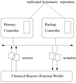
For example, consider the process-control system shown in Fig. 1. A digital controller supports monitoring, control, and actuation of a chemical reactor. The controller software executes a tight loop, sampling sensors, calculating new values, and sending signals to external devices under its control. It also maintains an in-memory data repository which is updated frequently during each iteration of the control loop. The data repository must be replicated on a backup controller to meet the strict timing constraint on system recovery when the primary controller fails. In the event of a primary failure, the system must switch to the backup node within a few hundred milliseconds. Since there can be hundreds of updates to the data repository during each iteration of the control loop, it is impractical and perhaps impossible to update the backup synchro-nously each time the primary repository changes.

One class of weak consistency semantics that is particu-larly relevant in a real-time environment is temporal consistency, which is the consistency view seen from the perspective of the time continuum. Two objects or events are said to be temporally consistent with each other if their corresponding timestamps are within a prespecified

bound. Two common types of temporal consistency are: external temporal consistency, which deals with the relation-ship between an object of the external world and its image on the servers, and interobject temporal consistency, which concerns the relationship between different objects or events. Both consistencies stem from requirements by real world tasks. For example, when tracking the position of a plane, the data in the computer system must change within

some time bound (external temporal consistency) after the plane changes its physical position. When two planes approach the same airport, the traffic control system must update the positions of the two planes (interobject temporal consistency) within a bounded time window to ensure that the airplanes are at a safe distance from each other.

This paper presents a real-time primary-backup (RTPB) replication scheme that extends the traditional primary-backup scheme to the real-time environment. It enforces a temporal consistency among the replicated data copies to facilitate fast response to client requests and reduced system overhead in maintaining the redundant compo-nents. The design and implementation of the RTPB combines fault-tolerant protocols, real time task scheduling, (external and interobject) temporal data consistency, opti-mization in minimizing primary-backup temporal distance or primary CPU time in maintaining a given bound on such distance, deterministic or probabilistic consistency guaran-tee, and flexible x-kernel architecture to accommodate various system requirements. This work extends the Window Consistent Replication first introduced by Mehra et al. [25]. The implementation is built within the x-kernel architecture on MK7.2 microkernel from the Open Group.1

We chose passive replication because it provides faster response to client requests since no agreement protocol is executed to ensure atomic ordered delivery. Furthermore, it is also simpler and we want to experiment with new concepts on a simple platform before extending it to more complex architecture. In fact, the RTPB is part of our ongoing research on the application of weaker consistency models to replica management. In a recent tech report, we have examined a real-time active replication scheme with a similar consistency model as the RTPB.

The rest of the paper is organized as follows: Section 2 describes the RTPB model. Sections 3 and 4 define the concepts of external and interobject temporal consistency, respectively. Section 5 explores the optimization problem. Section 6 analyzes the failover process of the RTPB. Section 7 addresses implementation issues in our experience of building a prototype RTPB replication system, followed by a detailed performance analysis in Section 8. Section 9 summarizes the related work. Section 10 is the conclusion.

2 S

M

A

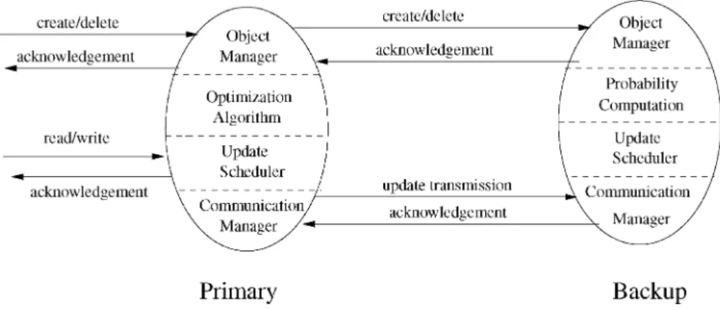
The proposed RTPB system consists of one primary and one or more backups. The primary interacts with clients and is responsible for keeping the backup(s) in weak consistency using the temporal consistency model developed in this paper. Unlike the traditional primary-backup protocols, the RTPB model decouples client write operations from com-munication within the service, i.e., the updates at backup(s). Furthermore, external and interobject temporal consistency semantics are defined and guaranteed at both the primary and backup sites by careful coordination of the operations at the primary and updates to the backups. Fig. 2 depicts the composition of the servers.

Fig. 1. A replicated process control system

1. Open Group is formerly known as the Open Software Foundation (OSF).

As shown in the figure, the primary's object manager handles client data requests and determines its merit, the update scheduler handles writes of the objects in the system, and the communication manager sends messages to the backups at the behest of the update scheduler. The optimization daemon in the primary handles the optimiza-tion of the RTPB while the probability calculaoptimiza-tion daemon in the backup module computes the probability of temporal consistency of the backup and is used to ensure a probabilistic consistent failover in case of primary failure. Since read and write operations do not trigger transmis-sions to the backup hosts, client response time depends only on local operations at the primary, which can be handled much more effectively. This allows the primary to handle a high rate of client requests while independently sending update messages to the backup replicas.

A client task periodically updates objects on the primary. The update must satisfy the external and interobject temporal constraint imposed on all objects in the system. The primary balances the demands of the client applica-tion's processing and the maintenance of consistent backup replicas by selectively transmitting messages to the back-up(s). The primary goal of the RTPB is to determine the frequency at which updates are sent to the backup such that the balance is achieved. The primary executes an admission control algorithm as part of object creation to ensure that the update scheduler can schedule sufficient update transmis-sions for any new object admitted such that the required temporal consistency is achieved. Unlike client reads and writes, object creation and deletion requires complete agreement between the primary and all the backups.

The RTPB system is designed to run under various system conditions and can tolerate a wide range of faults. We assume that processes can suffer crash or performance failures. (We don't assume Byzantine or arbitrary failures.) Send omissions and receive omissions are also allowed, e.g., due to transient link failures, or discard by the receiver due to corruption or buffet overflow. Permanent link failures (resulting in network partitions) are not considered. We believe that the proper way to handle permanent failures in fault-tolerant real-time systems is to employ hardware redundancy such as in TTP [16] or as suggested in [6].

If the fault mode is deterministic, i.e., the pattern and probability of a fault occurring is known or can be bounded

due to support by the underlying communication infra-structure, the RTPB can exploit this feature to provide deterministic consistency guarantee for replicated data copies. If the fault mode is nondeterministic, i.e., the probability of a fault occurring is unknown or impossible to model, the RTPB can degrade its guarantee of temporal data consistency to be probabilistic.

3 E

T

C

External temporal consistency concerns the relationship between an object of the external world and its image on a server. The problem of enforcing a temporal bound on an object/image pair is essentially equivalent to that of enforcing such a bound between any two successive updates of the object on the server. If the maximum time gap between a version of an object on the server and the version of the object in the external world must be bounded by some , then the time gap between two successive updates of the object on the server must be bounded by

too, and vice versa. Hence, the problem of guaranteeing an object's external temporal consistency is transformed to that of guaranteeing a bound for the time gap between two successive updates of the object on the server. If we define timestampTP

i …t†; TiB…t†at timetto be the completion time

of the last update of object i before or at time t at the primary and backup, respectively, then the temporal consistency requirement stipulates that inequalities tÿ TP

i …t† i andtÿTiB…t† 0i hold at allt, where i and i0

are the external temporal constraints for objectiat primary and backup, respectively. The values of i and 0i are

specified by the target applications. Hence, our task becomes to find the conditions that make the above two inequalities hold at all times.

3.1 Consistency at Primary

Consistency at primary requires that inequalitytÿTP i …t†

iholds at all times. Lettingpiandeidenote the period and

the execution time of the task that updates object i at primary, we have:

Lemma 1.tÿTP

i …t† iifpi …i‡ei†=2.

Proof.In the worst case, a version of objectiat the primary could stay current for as long as2piÿeitime units before

the completion of the next update; hence, at any time instantt, we have: tÿTP i …t† 2piÿei2…i‡ei†=2ÿeiˆi u t

To derive a necessary and sufficient condition for ensuring external temporal consistency, we introduce the notion of phase variance.

Definition 1.The kth phase variancevk

i of a task is the absolute

difference between the time gap of its kth and (kÿ1)th completion time, and its periodpi, i.e.,

vk

i ˆ j…fikÿfikÿ1† ÿpij; kˆ1;2;. . .;1:

Definition 2.Thephase varianceviof a task is the maximum

of its kth phase variance, i.e.,viˆmax…vi1; v2i; v3i;. . .†.

Since any two consecutive completion times of a periodic task is bounded between ei and 2piÿei, it follows

immediately from the definition of phase variance that:

viˆmax…j…fikÿfikÿ1† ÿpij† piÿei …3:1†

With the introduction of phase variance, we derive a necessary and sufficient condition for guaranteeing external temporal consistency for objectiat primary:

Theorem 1.tÿTP

i …t† i iffpiiÿvi.

Due to space limitation, we omit the proof here. Refer to http://www.eecs.umich.edu/~zou/paper/tpds.ps for proofs of all subsequent theorems in this paper.

3.1.1 Bound on Phase Variance

The result of Theorem 1 is of little use if phase variance can not be bounded by a bound that is better than the one given by (3.1). Fortunately, we are able to derive better bounds on phase variance for various scheduling algorithms:

Theorem 2. Phase variance is bounded by inequalities vi

xpiÿei under Earliest Deadline First (EDF) [23] scheduling,

by inequality vi …x:pi†=…n…21=nÿ1†† ÿei under

Rate-Monotonic Scheduling (RMS) [23], and by inequality vi

Riÿei under Response Time Analysis [8], [33] scheduling.2

Here, n is the number of tasks on the processor, x is the utilization rate, and Ri is the response time of the task that

updates objecti.

The Response Time Analysis approach provides a tighter bound on phase variance than RMS if the response time of each task is shorter than its corresponding period. We included RMS in our analysis because of its wide use in practice. We also note that if a task runs less than its worst case execution time, the bound on phase variance is looser, which will affect the temporal consistency guarantees. But such a problem can be addressed by using the best execution time in the above formulae.

From Theorems 1 and 2, we conclude that the restriction on an object can be significantly relaxed if the utilization rate of a task set is known. It can also be shown that if the number of objects whose external temporal consistency we want to guarantee is less than the number of tasks in the task set, the bound on phase variance can be further tightened. The formula that takes into account the number of objects for which we want to guarantee temporal consistency is straightforward to derive.

3.1.2 Zero Bound on Phase Variance

Thus far, we have demonstrated that phase variance can indeed be bounded by some known number. In fact, we can ensure that the phase variance is exactly zero in most cases through a direct application of the schedulability results from Distant-Constrained Scheduling (DCS) [13]. The DCS algorithm is used to schedule real-time tasks in which consecutive executions of the same task must be bounded, i.e., the finish time for one execution is no more thantime units apart from the next execution. Consider a task set

T ˆT1; T2;. . .; Tn. Suppose ei and ci denote the execution

time and distance constraint of task Ti, respectively, and

any two finish of taskTiis bounded byci. Han and Lin [13]

have shown that the task set can be feasibly scheduled under schedulerSr ifPniˆ1ei=cin…21=nÿ1†.

If we substitute pi for ci, then each finish of task Ti

occurs at exactly the same intervalpiafter some number of

iterations (could be 0). This can be proven by contra-diction: If the completion time of consecutive invocations is not exactly pi apart, then the difference between two

consecutive completion times must become smaller and smaller as time advances (because no two completion times can be more thanpi apart). Eventually, there will be

at least two consecutive completion times within a single period, which is impossible. Thus, the phase variance of task Ti in this case is j…fikÿfikÿ1† ÿpij ˆ jpiÿpij ˆ0.

Combining with the result of Theorem 1, we conclude that if Pn_iˆ1ei=pin…21=nÿ1†, the condition to guarantee

external temporal consistency for an object is relaxed to that of ensuring that the period of the task updating the object is bounded by the external temporal constraint placed on the object.

3.2 Consistency at Backup

The temporal consistency at the backup site is maintained by the primary's timely sending of update messages to the backup. Our interest here is to find out at what frequency the primary should schedule update messages to the backup such that inequality tÿTB

i …t† i0 holds at all

times. Let p0

i, e0i, and v0i denote the period, the execution

time, and the phase variance of the task that updates objecti

at backup, respectively, and`is the communication delay from primary to backup. We have:

Theorem 3. A sufficient condition for guaranteeing external

temporal consistency for object i at backup is

p0

i …0i‡ei‡e0iÿ`†=2ÿpi. A necessary and sufficient

condition for such guarantee isp0

i0iÿv0iÿpiÿviÿ`. 2. An exposition of scheduling algorithms is beyond the scope of this paper;

If we choose pi to be the largest value that satisfies the

external temporal constraint of objectiat the primary, i.e.,

pi ˆiÿvi, we obtain:

p0

i0iÿv0iÿ …iÿvi† ÿviÿ`ˆ …0iÿi† ÿv0iÿ`:

Moreover, if v0

iˆ0, the above formula is simplified to

p0

i …0iÿi† ÿ`. Letdenote0iÿi. We see that in order to

guarantee external temporal consistency for object iat the backup, an update message from the primary to the backup must be sent within the next ÿ` time units after the completion of each update on the primary. This is identical to the window-consistent protocol proposed by Mehra et. al. [25]. Here,is the window of inconsistency (or window consistent bound) between the primary and backup.

4 I

T

C

Interobject temporal consistency concerns the relationship between different objects or events. If one object is related to another in a temporal sense, then a temporal constraint between the two objects must be maintained. For example, when two planes approach the same airport, the traffic control system must update the positions of the two planes within a bounded time window to ensure that the airplanes are at a safe distance from each other. Ifijis the interobject

temporal constraint between objecti andj, the interobject temporal consistency requires that inequalities jTP

j …t† ÿ

TP

i …t†j ij andjTjB…t† ÿTiB…t†j ij hold at all times.

Theorem 4. A necessary and sufficient condition to guarantee interobject temporal consistency between object i and j is piijÿvi,pjijÿvjat primary, andp0iijÿv0i,p0j

ijÿv0jat backup.

The correctness of the theorem is intuitive. Since any two consecutive completion times of one task that meet the condition are bound by the temporal constraint, any two neighboring completion times of two tasks that meet the same condition are bound by the temporal constraint, too.

If the phase variances in the above formulae are made zero by DCS scheduling, then the conditions stated in Theorem 4 are simplified to:

piij;andpjijfor the primary

p0

iij;andp0jijfor the backup

which means that the interobject temporal constraint between object i and j at both the primary and backup can be maintained by scheduling the two updates (for objects i and j, respectively) within a bound of ij time

units.

5 O

The previous two sections developed conditions that ensure temporal consistency for any object in the system. Such consistency effectively bounds the temporal distance (time-stamp difference) between an object on the primary and the corresponding copy on the backup. However, the discus-sion does not minimize such a distance nor the primary's CPU overhead used in maintaining a given bound on it.

This section explores ways to optimize the system from these two perspectives.

5.1 Definitions

First, we define temporal distance. If we timestamp each data copy on both the primary and backup, then at any given time instantt, the difference between the timestamp of object iat the primary and the timestamp of the same object at the backup is thetemporal distanceof objectiin the system. We define the overalltemporal distanceof the system to be the arithmetic average of the temporal distance of each object.

Definition 3. The temporal distance for object i at time t is

jTP

i …t† ÿTiB…t†j. The overall temporal distance of the system

at time t is Pn

iˆ1jTiP…t† ÿTiB…t†j=n, where n is the total

number of objects registered in the replication service. From another perspective, temporal distance can be seen as the data inconsistency for object ibetween the primary and the backup. The overall temporal distance can therefore be seen as the overall data inconsistency of the system. If the overall temporal distance is within some prespecified, we call the backup temporally consistent with respect to the primary. The definition oftemporal distancealso suggests a way to compute its value. To compute the temporal distance for a single object iat any time, we need to find out the time instants at which objectiwas last updated on the primary and backup and take the absolute difference of these two timestamps. To compute the overall temporal distance of the system at any time, we compute the temporal distance for each object and take their arithmetic average.

5.2 Minimizing Temporal Distance

Observe that the more frequently updates are sent to backup, the smaller the temporal distance will be. Thus, if the period of the updates sent to backup for each object is minimized, the overall temporal distance between the primary and backup is also minimized. Furthermore, the minimization of the update period at the backup for each object results in the minimization of the sum of the update periods for all objects and vice versa. Hence, our first attempt is to use the sum of the update periods for all objects as our objective function. Then the optimization problem can be stated as:

minimize: Pp0 i

subject to: Pn_iˆ1…e0

i=p0i‡ei=pi† 2n…21=2nÿ1†

and pip0i0i; iˆ1;2;. . .; n

The first constraint ensures task schedulability under both RMS [23]and DCS [13]. But the optimization problem can also be phased to use other scheduling algorithms. For example, if we use EDF, this constraint is changed to P_n

iˆ1…e0i=pi0‡ei=pi† 1. If we use Response Time Analysis

[8], [33], the constraint is changed to

8i; e0 i‡ X j2hp…i† …dR0 i=p0jee0j‡ dRi0=pjeej† p0i;

where hp…i† denotes the set of tasks that have a higher priority than the task updating objecti. In our subsequent

discussions, we only use RMS and DCS scheduling for the reason that RMS is the most commonly used scheduling algorithm in practice, while DCS can provide a tight bound on phase variance.

The inequality p0

ii0 ensures that the temporal

con-straint imposed on object i at the backup is maintained, while inequality pip0i guarantees that no unnecessary

update is sent to the backup since more frequent updates at backup would not make any difference when there is no message loss between servers. However, such formulation of the optimization problem is not very useful in practice because it is not in a normalized form and the solutions to it are skewed towards the boundaries. In other words, for most objects (actually all objects except one), the period is either very high or very low, which means for certain objects, the respective temporal distances between primary and backup are not optimized at all. For example, if we have four objects in the system with

eiˆe0iˆ f1;2;3;4g;

piˆ f10;20;30;40g;

0

iˆ f50;50;60;70g;

respectively, then the minimization of Pp0

i is achieved

if p0

iˆ f50;20;30;40g. All values in the p0i vector are on

the boundaries (skewed solution) in the constrainting inequalities.

In fact, we can show that if an optimal solution exists for the above optimization problem, there is exactly one object that has its period strictly bounded between the boundaries given in the constraining inequalities. Indeed, we can generalize this observation to the following theorem: Theorem 5. The optimal solution in minimizing Pn_iˆ1cixi

subject toPn_iˆ1aixib,lixi uiiˆ1;. . .; nhas at most

one of the variables bounded strictly between its lower and upper boundaries.

This analysis necessitates a need to find a normalized objective function whose solutions are not skewed toward any extreme. One suitable alternative is the maximization of min…p1=p01; p2=p02;. . .; pn=p0n†. This objective function is

simple and its solution can be easily found by a polynomial time algorithm. Furthermore, all the periods are propor-tionally made as small as possible without skew. Now the optimization problem can be formulated as:

maximize: min…p1=p0

1; p2=p02;. . .; pn=p0n†

subject to: Pn

iˆ1…e0i=p0i‡ei=pi† 2n…21=2nÿ1†

and pip0ii0; iˆ1;2;. . .; n

The proof that the above function indeed minimizes temporal distance is beyond the scope of this paper. However, its correctness can be explained intuitively as follows: Since the maximization of the minimum of…pi=p0i†

minimizes the update transmission periodp0

iproportionally

to its corresponding update period at the primary, the overall update frequency at the backup is therefore proportionally maximized, which results in the minimiza-tion of temporal distance.

The above formulation states that to minimize temporal distance, one needs to minimize the maximum period of the

update tasks for the object set subject to both schedulability and temporal constraint tests. We distinguish betweenstatic

and dynamic allocation in designing a polynomial time

algorithm that achieves this objective. Static allocation deals with the case where the set of objects to be registered are known ahead of time. The goal is to assign the update scheduling period for each object such that the value of the object function is maximized. Dynamic allocation deals with the case where a new object is waiting to be registered in a running system in which a set of objects have already been registered.

5.2.1 Static Allocation

Since all objects are know a priori, the algorithm for scheduling updates from primary to backup is relatively straightforward:

1. Assignp0

i ˆ0i initially

2. Perform schedulability test using RMS [23] or DCS [13]. If it fails, then it is impossible to schedule the task set without violating the given temporal constraint.

3. Otherwise, sort termspi=p0i into ascending order.

4. Shorten periodp0

iof the first term in the ordered list until

it either becomes the second smallest term, or reaches the lower boundpi, or the utilization rate of the whole task set

is saturated.

5. Repeat steps 3-4 until the utilization becomes saturated or all ratios become 1.

Note that steps 3-4 can be implemented efficiently by binary insertion which is bounded bylogn, and the running time of the algorithm is dominated by the number of iterations of steps 3-4, which is bounded by

…max…pi=p0i† ÿmin…pi=p0i††2;

the total running time of the algorithm is

O……max…pi=p0i† ÿmin…pi=p0i††2logn†:

5.2.2 Dynamic Allocation

A new object is being registered with a system in which other objects have already been checked in. We want to find out if the new object can be admitted and at what frequency we can optimally schedule its update task. We can pursue either a local optimum or global optimum with the difference being that local optimum algorithm does not adjust the periods of tasks that are already admitted and global optimum algorithm considers all tasks in devising an optimal scheduling.

Local optimal

1. Assign the smallest value that ispibut0ito the new

task such that the total utilization of the task set is still under2n…21=2n_{ÿ1† (this ensures that the whole task set is}

schedulable under RMS and DCS). 2. If step 1 fails, then reject the new object. Global optimal

1. Insert termpi=p0i into the ordered list that we obtained in

2. Rerun the static allocation algorithm. 3. If step 2 fails, then reject the new object.

The running time for local optimum algorithm is linear (with respect to the number of objects). The time complexity for the global optimum algorithm is the same as that of the static allocation algorithm which is polynomial.

5.3 Minimizing Primary CPU Overhead

This section discusses the optimization problem of mini-mizing primary CPU time used in scheduling updates to the backup. The observation is that the less frequently updates are sent to backup, the less primary CPU overhead will be. Hence, the minimization of primary CPU overhead can be achieved by minimizing the number of updates sent to the backup, which is equivalent to the maximization of the periods of the update tasks (under the given temporal distance bound). We assume that the transmission of an update message of any object takes the same amount of primary CPU time.

Note that the bound on temporal distance can be converted to a bound on the periods of the updating tasks. If we normalize the period of each update task with the denominatoriÿpi, the given bound on temporal distance

can be transformed to inequalityPp0

i=…iÿpi† B, where

B is some positive constant derived from the given constraint on temporal distance. Observe that we do not need to know the actual value of B. The important thing here is thatBcan be derived from the bound on temporal distance. Thus, our optimization can be formulated as: maximize: Pn_iˆ1p0

i

subject to: Pn_iˆ1p0

i=…iÿpi† B

and pip0i0i

The following is a polynomial time algorithm for the problem:

1. For each object, assign period:p0 iˆ0i.

2. Perform schedulability test. If the test fails, then we cannot guarantee the temporal consistency of the object set. Reject the object set.

3. Otherwise, computeXˆPp0

i=…iÿpi†.

4. IfXB, then we are successful. So we stop here. 5. Shorten thep0

is proportionally such that the value of the

summation is reduced by the amount ofXÿB.

6. Perform schedulability test again. If it fails, then reject the object set. Otherwise, we have succeeded in devising an optimal scheduling.

The rationale behind the algorithm is that to minimize primary CPU overhead in maintaining the given temporal bound on temporal distance, we simply schedule as few updates to the backup as possible for each object subject to the individual temporal constraint and the overall temporal distance bound. The running time of the above algorithm is linear.

If we relax the value0

isuch that it can be unbounded, i.e.

we take out the constraint p0

i 0i, the problem becomes

intractable. If fact, we have: Theorem 6. maximizing Pn

iˆ1p0i under constraint

P_n

iˆ1p0i=…iÿpi† Bis NP-complete.

5.4 Optimization under Message Loss

The discussion on RTPB optimization so far does not take into consideration message loss. Update messages from primary to backup can be lost due to sender omission, receiver omission, or link failure. This section devises a modified scheduling protocol that takes into account message loss. We define the probability of a message loss from primary to the backup to be, and the probability of the temporal consistency guarantee we want to achieve to beP. Then for an update to reach backup with probability

P, the number of transmissions needed islog…1ÿP†=log…†. Hence, the problem of minimizing temporal distance of the system can be formulated as:

maximize: min……pilog…††=…p0ilog…1ÿP†††

subject to: Pn_iˆ1…e0

i=p0i‡ei=pi† 2n…21=2nÿ1†

and …pilog…††=log…1ÿP† p0i0i

The goal is to send updates to the backup more frequently in case of a message loss. The frequency of update transmissions can be increased up to the frequency at which any update will reach the backup with probability

P. The maximization of the minimum term in the objective function results in the overall minimization of periods of the update tasks, which consequently results in the minimiza-tion of temporal distance with probability P. The con-straints in the formulation ensure schedulability while maintaining temporal consistency for each individual object and avoiding unnecessary updates to the backup. With proper substitution of terms, the same algorithm introduced before can be applied here. Due to space limitations, we omit it.

Similarly, the minimization of primary CPU overhead in maintaining a given bound on temporal distance when message loss occurs becomes:

maximize: Pn_iˆ1p0 i subject to: Pn_iˆ1p0 ilog…1ÿP†=‰log…iÿpi†Š B and p0 i0ilog…†=log…1ÿP†

Again, the algorithm in the previous section can be used here with proper parameter substitution.

6 F

RTPB

A failover occurs when the backup detects a primary failure. In such a case, the backup initiates a failover protocol and takes over the role of the primary with the necessary state updates and notification of clients. There are two aspects concerning a failover: the qualitative aspect and the quantitative aspect. The former deals with the question of ªhowº to detect a failure and ªrecoverº from it. The latter deals with the two quantitative aspects of a failover: failover consistency and failure recovery time.

The approach to failure detection and recovery is to let the replicas exchange periodic pingmessages. Each server acknowledges the ping message from the other one. If a server receives no acknowledgment over some time, it will timeout and resend apingmessage. If there is no response beyond a certain amount of time, the server will declare the other end dead. When the primary detects a failure on the

backup, nothing happens to the clients since the primary only cancels the update transmissions to the backup while its service to clients continues uninterrupted. If the backup detects a crash in the primary, it initiates a failover protocol in which it notifies the clients of such an event, modifies the necessary system parameters to reflect this change, and starts to serve clients.

The quantitative aspect of a failover concerns two questions. The first question is: Is the new primary after a failover procedure temporally consistent with respect to the old primary immediately before its crash? If we can't answer this question for certain, can we compute the probability that once the failover is complete, the new primary is temporally consistent? Such a question is legitimate because it is important for us to know the state of the new primary after a failover so that we can assess the quality level of its service and take proper measures if necessary. The second question is: How long does it take for a failover procedure to complete? A timing measurement for the recovery is important because we want to minimize the impact of a failure on the clients. We address the two aspects separately below.

6.1 Probability of Failover Consistency

The probability of failover consistency concerns the like-lihood that upon the completion of a failover, the new primary (old backup) is temporally consistent with respect to all the objects of the old primary at the time of its crash. It is straightforward to see that the probability of a consistent failover is equivalent to the probability of backup consis-tency at the time when the failover starts. Suppose the backup detects a primary failure at time t, then the probability that the backup is temporally consistent with respect to the old primary at timetis what we are looking for.

If everything works properly, then RTPB ensures that the backup is temporally consistent with respect to the primary at all times. So the probability of failover consistency is1. However, in case of random faults where messages can be lost with unknown probability, the calculation of temporal consistency of the backup at any point in time t becomes important. Ifti

uis the timestamp of the last update for object

ion the backup before timet, then the probability that the backup's copy of object ifalls out of temporal consistency with its counterpart on the primary at time t is the probability that an update occurred at the primary during time interval ‰ti

u; tÿŠ, where is the temporal constraint

between primary and backup. We should note that if ti

utÿ, then there could not

have been any update occurring at the primary for objecti

during the time interval in question. Hence, the probability of temporal consistency of the backup with respect to object

i is 1. If ti

u‡pitÿ, then it is certain that an update

occurred at the primary because the update at the primary is periodic with period pi. Hence, the probability of

temporal consistency of the backup with respect to object

iis0.

Otherwise, since the primary updates its object periodi-cally and the update is random and uniformly distributed within each period, the probability of an update for objecti

occurring at the primary during time interval ‰ti

u; tÿŠ is

…tÿÿti

u†=pi. Thus, the probability that the backup is

temporally consistent with respect to object i at time t is 1ÿ …tÿÿti

u†=pi. LettingPi…t†denote such probability, we

have: Pi…t† ˆ 1 tÿti u 0 tÿti u‡pi 1ÿ …tÿÿti u†=pi otherwise: 8 < : …6:1†

If there arenobjects in the system andP…t†denotes the probability that the backup is temporally consistent with respect to every object in the primary at time t, then we have:P…t† ˆQn_iˆ1Pi.

Now that we have derived the probability of temporal consistency of the backup at any given time instantt, we can determine the probability of a consistent failover. If the backup discovers that the primary is crashed at time t, it immediately takes over the role of the primary and starts to serve the clients. Assume the time it takes for the backup to declare its substitution as the new primary is negligible, then the probability of a consistent failover is the same as that of temporal consistency of the backup with respect to the old primary at timet, which can be computed according to (6.1).

6.2 Failure Recovery Time

The detection and recovery time from a primary crash is an important factor in determining the quality of a primary-backup replication system. The detection time is the time interval between the instant a server is crashed and the instant that the crash is detected. The recovery time is the time interval between the instant that a crash is detected and the instant that service is resumed.

The shortest time interval between a primary crash and the detection of this event by the backup is the number of maximum tries of sending thepingmessage by the backups minus 1, multiplied by round-trip latency2`. If the number of tries isn, then the shortest time of detection is2…nÿ1†`

and the longest time interval of detection is2n`. Hence, the failure detection timetd is bounded between2…nÿ1†`and 2n`. The recovery time is a little trickier to compute. In our design, after the detection of primary failure, the backup simply starts a backup version of the applications and up-loads the state information, and then starts to serve again. The major component of the recovery time is the time that it takes to upload the state information, which is dependent on the size of the state information. In general, the total detection and recovery time is dominated by the detection time. Therefore, we can use the upper bound of the detection time to approximate the failure detection and recovery time, which is2n`.

6.3 Probabilistic RTPB

We can use the probability computation described in the previous sections to build a modified RTPB that provides a probabilistic data consistency guarantee when the primary fails. Since the computation of the probability of backup consistency is independent of the fault patterns of the communication substructure, such a consistency guarantee holds regardless of the service provided by the lower layers. To achieve such a guarantee, the backup needs to perform

an additional task when primary failure is detected. Before initiating the failover process, the backup computes the probability of its temporal consistency with respect to the primary immediately before crash and takes one of the following two actions depending on the requirement imposed by the applications.

If a probability threshold is specified by the application, the backup, after becoming the new primary, automatically denies service to clients if the probability of consistency computed is less than the given threshold and resumes services only after new updates are received. Hence, if the client receives a service, it can be assured that the service is temporally consistent with the probability of at least the given threshold. If no probability threshold is given, then the backup simply notifies the clients of the probability of temporal consistency and lets the clients determine the goodness of the service.

7 P

I

7.1 Environment and Configuration

Our system is implemented as a user-levelx-kernel-based server on the MK 7.2 microkernel from the Open Group. Thex-kernel is a protocol development environment which explicitly implements the protocol graph [14]. The protocol objects communicate with each other through a set of x -kernel uniform protocol interfaces. A given instance of the

x-kernel can be configured by specifying a protocol graph in the configuration file. A protocol graph declares the protocol objects to be included in a given instance of thex -kernel and their relationships.

We chose the x-kernel as the implementation environ-ment because of its several unique features. First, it provides an architecture for building and composing network protocols. Its object-oriented framework promotes reuse by allowing construction of a large network software system from smaller building blocks. Second, it has the capability of dynamically configuring the network software, which allows application programmers to configure the right combination of protocols for their applications. Third, its dynamic architecture can adapt more quickly to changes in the underlying network technology [27].

Our system includes a primary server and a backup server which are hosted on different machines that are connected by a 100MB fast ethernet. Both machines maintain an identical copy of the client application.3

Normally, only the client on the primary is active, while the client copy on the backup host is dormant. The client continuously senses the environment and periodically sends updates to the primary. The client accesses the server using Mach IPC-based interface (cross-domain remote procedure call). The primary is responsible for backing up the data on the backup site and limiting the inconsistency of the data between the two sites within some specified

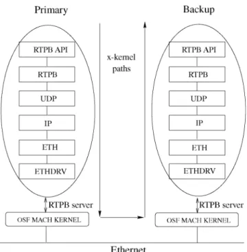
window. Fig. 3 shows the RTPB system architecture andx -kernel protocol stack.

At the top level is the RTPB application programming interface, which is used to connect the outside clients to the Mach server on one end and Mach server to thex-kernel on the other end. Our real-time primary-backup (RTPB) protocol sits right below the RTPB API layer. It serves as an anchor protocol in the x-kernel protocol stack. From above, it provides an interface between thex-kernel and the outside host operating system, OSF Mach in our case. From below, it connects with the rest of the protocol stack through the x-kernel uniform protocol interface. The underlying transport protocol is UDP. Since UDP does not provide reliable delivery of messages, we need to use explicit acknowledgments when necessary.

The primary host interacts with the backup host through the underlying RTPB protocol that is implemented inside the x-kernel protocol stack (on top of UDP, as shown in Fig. 3). There are two identical versions of the client application residing on the primary and backup hosts respectively. Normally, only the primary client application is running. But, when the backup takes over in case of primary failure, it also activates the backup client applica-tion and brings it up to the most recent state. The client application interacts with the RTPB system through the Mach API interface we developed for the system.

7.2 Admission Control

Before a client starts to send updates of a data object to the primary periodically, it first registers the object with the service so that the primary can perform admission control to decide whether to admit the object into the service. During registration, the client reserves the necessary space for the object on the primary server and on the backup server. In addition, the client specifies the period it will update the object pi as well as the temporal constraint

allowed for the object on both the primary site and the backup site, where the temporal constraint specified by the client is relative to the external world. The consistency window between the external data objectiand its copy on the primary isi. Because primary's copy of objectichanges

only when the client sends a new update, the inconsistency between the external data and its image on the primary is dependent on the frequency of client updates. Hence, it is the responsibility of the client to send updates frequently enough to make sure the primary has a fresh copy of the data.

The primary compares the value ofi and pi. Ifpii,

then the inconsistency between the external data and the primary copy will always fall into the specified consistency window. If the condition does not hold, the primary will not admit the object. The primary can provide feedback so that the client can negotiate for an alternative quality of service. Given the temporal constraint for objection the primary

i and the constraint on the backup 0i, the consistency

window for object ibetween the primary and the backup can be calculated as 0

iÿi. Let ` be the average

commu-nication delay between the primary and the backup. If the consistency window is less than`, then it is impossible to maintain consistency between the primary and backup servers. Therefore, during the registration of object i, the

3. The RTPB model allows stand alone clients as well as clients that run on the same machine as the server replicas. What we mean by client here is the code that reads/modifies the data objects. One can view the latter mode as replicating the application that accesses the data objects. The current implementation supports this mode of operation, i.e., the client application runs on the RTPB servers. The implementation can be easily modified to handle requests from remote clients.

primary will check if relation0

iÿi> `holds for objecti. If

the relation does not hold, the primary rejects the object. After testing that the temporal consistency constraints hold for objecti, the primary needs to further check if it can schedule a periodic update event (to the backup) for objecti

that will meet the consistency constraint of the object on the backup without violating the consistency constraints of all existing objects. For example, the primary will perform a schedulability test based on the rate-monotonic scheduling algorithm [23]. If all existing update tasks as well as the newly added update task for object iare schedulable, the test is successful. Otherwise, the object is rejected.

Each interobject temporal constraint is converted into two external temporal constraints according to the results derived in Section 4. Specifically, given objectsiandjand their interobject temporal constraint ij, their interobject

temporal bound can be met at the primary if piij,

pjij, and the schedulability test are successful. This same

constraint can be met at the backup as long as the constraint

ij is sufficiently large such that the primary can schedule

two new update tasks that periodically send update messages to the backup without violating the temporal constraints of any existing object that is registered with the replication service.

After both the schedulability and temporal constraint tests, the primary also needs to perform a network bandwidth requirement test. The primary computes the system's bandwidth requirement B, using a number of parameters including the number of objects, their sizes, and the frequency at which updates for these objects are sent to the backup. Then it compares the value of B with the available network bandwidth to the system. If B is satisfiable, the object is admitted; otherwise it is rejected.

7.3 Update Scheduling

In our model, client updates are decoupled from the updates to the backup. The primary needs to send updates to the backup periodically for all objects admitted in the service. It is important to schedule sufficient update transmissions to the backup for each object in order to control the inconsistency between the primary and the backup. In the absence of link failures, ` is the average communication delay between the primary and the backup. For external temporal constraint, if a client modifies an objecti, the primary must send an update for the object to the backup within the next0

iÿiÿ`time units; otherwise,

the object on the backup may fall out of the consistency window. In order to maintain the given bound of the data inconsistency for object i, it is sufficient that the primary send an update for objectito the backup at least once every

0

iÿiÿ` time units. Because UDP, the underlying

trans-port protocol we use, does not provide reliability of message delivery, we build enough slack such that the primary can retransmit updates to the backup to compen-sate for potential message loss. For example, we set the period for the update task of objectias…0

iÿiÿ`†=2in our

experiments. For interobject temporal constraint, the pri-mary simply schedules the two updates for object iand j

withinij time units (see Section 4).

The optimization techniques can be easily embedded in our implementation. If the minimization of temporal distance is desired, then the algorithm described in the section concerning temporal distance is used to schedule updates from the primary to the backup in which case the frequency of updates being sent to backup for each object is increased proportionally until the primary CPU is fully utilized. If the minimization of primary CPU overhead used in maintaining the given bound on temporal distance is sought, then the algorithm discussed in the section concerning CPU usage is applied. But in either of these cases, if a client modifies an objecti, the primary must send at least one update for the object to the backup within the next 0

iÿiÿ` time units; otherwise, the object on the

backup may fall out of the consistency window. If the probability of message loss from the primary to the backup and the probability to achieve guarantees of the temporal consistency in the system are given, then we apply the optimization technique that deals with message loss.

8 S

P

This section summarizes the results of a detailed perfor-mance evaluation of the RTPB replication system intro-duced in this paper. The prototype evaluation considers several performance metrics:

. Response time with/without admission control. . Temporal distance between primary and backup. . Average duration of backup inconsistency. . Probability of failover consistency.

. Failure recovery time.

These metrics are influenced by several parameters including client write rate, number of objects being accepted, window size (temporal constraint between primary and backup), communication failure, and optimization. All Fig. 3. System architecture and protocol stack.

graphs in this section illustrate both the external and inter-object temporal consistency. Each interinter-object temporal constraint is converted into two external temporal con-straints with the external temporal constraint being replaced by the interobject temporal constraint.

8.1 Client Response Time within RTPB

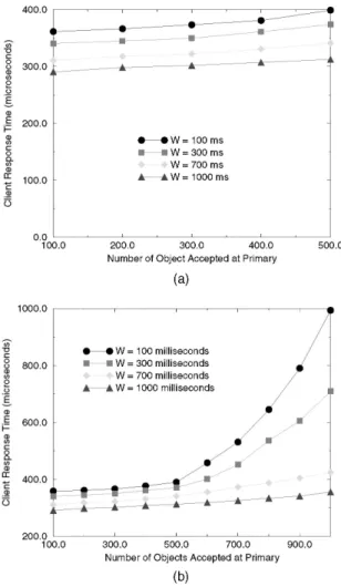
This metric measures the average response time to client requests by RTPB. To show that our admission control process is functioning correctly, we measured the metric under two different conditions with and without admission control. Fig. 4 shows the client response time as a function of the number of objects being accepted by the system. Fig. 4a shows the situation when the admission control is enabled in the primary and Fig. 4b shows the case when such process is disabled.

As shown in the graph in Fig. 4a, the number of objects has little impact on the response time of the system. This is due to the fact that the admission control in the primary acts as a gatekeeper that prevents too many objects from being admitted. The decoupling of client updates from backup updates is also a major contributing factor. The graph in Fig. 4b shows that the number of objects has little impact on the response time of the system when it is within the allowable limit of the window size. But the response time increases dramatically if the number of objects exceeds the

maximum allowable number of objects under a given window size. By disabling admission control, the number of objects accepted into the system can go out of control, which consequently degrades system performance.

For the same number of objects, larger client update periods have a better response time regardless of the enabling or disabling of admission control in the primary. The larger the client update period, the more leeway the primary has (due to the decoupling in RTPB) in scheduling update messages to the backup. Hence, the primary is able to schedule local updates and client responses while delaying transmission of updates to the backup. Note that we did not show the effect of optimization on the response time. The impact of optimization is insignificant in this regard because the unoptimized RTPB already schedules close to minimum number of updates to the backup. So there is not much room left for improving response time by reducing the number of updates sent to the backup (which increases available resources at the primary for client request processing).

8.2 Primary-Backup Temporal Distance

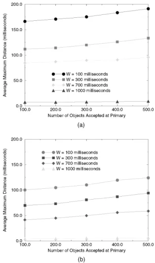
This metric measures the average maximum temporal distance between the primary and the backup. As the system runs, we take a snapshot of the system at regular time intervals, find the timestamps of the objects at the primary and backup, get the difference of the timestamp for each object between primary and backup, and then sum them together to derive the average temporal distance between primary and backup. Fig. 5 shows the average temporal distance as a function of the probability of message loss from the primary to the backup. Fig. 5a shows the case when no optimization technique is used and Fig. 5b shows the situation when optimization is used. Both Figs. 5a and 5b illustrate average temporal distance for four client update rates of 100, 300, 700, and 1,000 milliseconds.

From the graph in Fig. 5a, we see that the average temporal distance between the primary and the backup is close to zero when there is no message loss. However, as the message loss rate goes up, the distance also increases. For example, when the message loss is 10 percent, the average temporal distance between the primary and the backup approaches 700 milliseconds for client update period of 1,000 milliseconds. In general, the distance increases as the message loss rate or client write rate increases. We observe from the graph in Fig. 5b that the optimization techniques bring about a 35 percent to 60 percent improvement on the average temporal distance between the primary and back-up. Furthermore, we note that the shape of the graph under optimization is much smoother than when no optimization is used because the effect of message loss is reduced by the scheduling method which compensates for message loss.

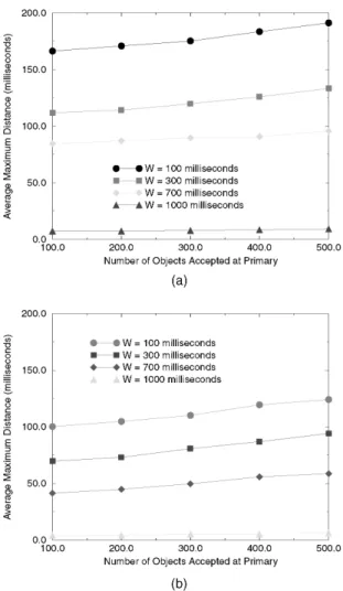
Fig. 6 compares the performance on the average temporal distance between the primary and backup with and without optimization as a function of the number of objects being accepted at primary. Again, we observe that the average temporal distance in the case where optimiza-tion techniques are used is about 40 percent to 60 percent smaller than that without optimization under the same set of parameters.

Fig. 4. Response time to client requests: (a) with admission control, (b) without admission control.

Optimization or no optimization, the set of graphs shows that in general, RTPB keeps the backup very close to the primary in terms of the temporal distance between the corresponding data copies of the replicated objects. Even without optimization, the largest temporal distance under normal operation (message loss is small or none) ranges from 160 to 190 milliseconds, which is well within the range that is tolerable by most real-time applications.

8.3 Duration of Backup Inconsistency

Another interesting metric measures the duration of inconsistency at the backup. We collect the data as described in the previous section and record the length of all continuous periods in which the backup falls out of the temporal constraint window between primary and backup. Fig. 7 shows the duration of backup inconsistency with and without optimization as a function of the probability of message loss between the primary and backup.

The figures show that whether or not optimization is used, the larger the probability of message loss, the longer the backup stays in an inconsistent state from the primary. Also, larger client update periods have shorter duration of backup inconsistency. If an update message is lost, the backup would stay inconsistent until the next update message comes. Since the frequency of an update message

is not determined by client write rate but by the capacity of the CPU resource at the primary, a larger client update period would mean a shorter duration of backup incon-sistency because the update frequency at the backup is higher than the update frequency at primary.

The optimization brings an order of magnitude improve-ment. The figures show that the optimized algorithm has a higher degree of tolerance to message loss. With optimiza-tion, there is no backup inconsistency until the message loss rate exceeds 6 percent. After that, the duration of incon-sistency increases slowly. But the test without optimization suffers backup inconsistency when the message loss rate is about 1 percent and after that the duration of inconsistency increases rapidly as message loss rate increases.

8.4 Probability of Failover Consistency

To measure this metric, we intentionally let the primary crash and then observe the behavior of the backup and measure the actual probability of the consistency of the failovers. Such probability is derived by actually counting the number of objects that are consistent and inconsistent and then dividing the number of consistent objects by the total number of objects in the system. This process is repeated many times to smooth out inaccuracies. The measurement is conducted under various conditions and Fig. 5. Temporal distance under message loss: (a) without optimization,

(b) with optimization.

Fig. 6. Primary-backup temporal distance: (a) without optimization, (b) with optimization.

parameters that include time of failure detection, temporal constraints, number of objects in the system, etc.

Fig. 8 measures the probability of failover consistency as a function of the time at which the failure is detected (measured as the difference between the time the last update at the backup occurred and the time at which primary failure is detected). The temporal constraint between the primary and backup for the system is set to 100 milliseconds. The graph plots the probability function for 100 objects with four different client update periods of 100, 300, 700, and 1,000 milliseconds, respectively.

The most important result is that it conforms to the result of our calculation according to the formula derived in Section 6. Second, the graph tells us that the earlier the detection of failure, the more likely the failover will be consistent. This makes sense since earlier detection means that the backup lags less far behind the primary at the time of such detection which in turn means that the backup is more likely to be temporally consistent than that of a later detection.

The graph also shows that the change of detection time has a dramatic effect on the probability of consistency. As the time of detection increases, the probability of consis-tency drops rapidly and quickly reaches zero and remains there afterward. The graph further shows that the more

frequently the updates are made at the primary, the less likely the failover will be temporally consistent. This again makes sense because more frequent updates at the primary make it harder for the backup to keep up with the system state and, hence, more likely to fall behind the primary, which means that the backup is less likely to be temporally consistent at the time of detection.

Fig. 9 measures the same metric but not as a function of time of detection. Instead, it is measured as a function of the temporal constraint placed on the system. This time, the time of detectiontÿtu is fixed at 1,000 milliseconds while

the temporal constraint between primary and backup varies from 100 to 1,000 milliseconds. Again, the graph is plotted for 100 objects with four different update periods at the primary.

From the graph, we observe that as the temporal constraint increases (loosens), the probability of failover consistency increases, which makes sense because consis-tency is inversely influenced by the constraint. The looser the constraint, the more likely that the backup is temporally consistent with the primary at any time and, hence, at the time of a primary crash. For the same temporal constraint, a larger update period at the primary has a higher probability of failover consistency. This makes sense because the less frequently the updates are at the primary, the easier the backup can keep up with the system state and, hence, the more likely the backup can stay in a consistent state given all other parameters being the same.

8.5 Failure Recovery Time

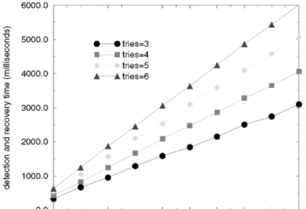
We have conducted extensive experiments to measure the failure detection and recovery time. Again, we deliberately let the primary crash and record the time at which the crash occurs. Then we observe the behavior of the backup and record the time at which service to clients is resumed. We then subtract the two time instants to get our failure detection and recovery time. Fig. 10 is the result of our measurement. The graph shows the metric as a function of theping period which specifies the time interval between two successive pingmessages. It is plotted for 500 objects with four different ªtryº variables which regulate the number of tries to sendpingmessage before declaring the other end dead.

Fig. 7. Duration of backup inconsistency: (a) without optimization, (b) with optimization.

The graph shows that the failure detection and recovery time increase as the ping period increases. This is because the longer the interval between two successive ping messages, the more time is needed to confirm a failure on the primary. Hence, the detection and recovery time is also longer. For the samepingperiod, the larger the number of tries, the longer the failure detection and recovery time. This is natural since a larger number of tries before declaring the other end dead means longer time for the detection. In general, the results indicate that the overall detection and recovery time can be made within half a second with proper parameter setting. For example, if we set ping period to 200 milliseconds and try number to 3, then the failure detection and recovery time is less than half of a second. This kind of recovery time is sufficiently fast for the majority of applications that are encountered in the real-time environment.

9 R

W

9.1 Replication Models

One can structure a distributed system as a collection of servers that provide services to outside clients or to other servers within the system. A common approach to building fault-tolerant distributed systems is to replicate servers that fail independently. The objective is to give the clients the illusion of service that is provided by a single server. The main approaches for structuring fault-tolerant servers are passiveandactivereplication. In passive replication schemes [3], [5], [7], the system state is maintained by a primary and one or more backup servers. The primary communicates its local state to the backups so that a backup can take over when a failure of the primary is detected. This architecture is commonly called the primary-backup approach and has been widely used in building commercial fault-tolerant systems. In active replication schemes [6], [10], [26], [30], [31], also known as thestate-machine approach, a collection of identical servers maintain replicated copies of the system state. Updates are applied atomically to all the replicas so that after detecting the failure of a server, the remaining servers continue the service. Schemes based on passive replication tend to require longer recovery time since a backup must execute an explicit recovery algorithm to take

over the role of the primary. Schemes based on active replication, however, tend to have more overhead in responding to client requests since an agreement protocol must be run to ensure atomic ordered delivery of messages to all replicas.

Past work on synchronous and asynchronous replication protocols has focused, in most cases, on applications for which timing predictability is not a key requirement. Real-time applications, however, operate under strict timing and dependability constraints that require the system to ensure timely delivery of services and to meet certain consistency constraints. Hence, the problem of server replication possesses additional challenges in a real-time environment. In recent years, several experimental projects have begun to address the problem of replication in distributed hard real-time systems. For example, TTP [16] is a real-time-triggered distributed real-time system: Its architecture is based on the assumption that the worst-case load is determined a priori at design time and the system response to external events is cyclic at predetermined time-intervals. The TTP architecture provides fault tolerance by implementing active redun-dancy. A Fault-Tolerant Unit (FTU) in a TTP system consists of a collection of replicated components operating in active redundancy. A component, consisting of a node and its application software, relies on a number of hardware and software mechanisms for error detection to ensure a fail-silent behavior.

DELTA-4 [4] is a fault-tolerant system based on distribu-tion that provides a reliable networking infrastructure and a reliable group communication and replication management protocols to which computers of different makes and failure behavior can plug in. It also supplies an object-oriented application support environment that allows building application with incremental levels of fault tolerance while hiding from the programmer the task of ensuring depend-ability. The leader-follower model was used extensively in DELTA-4 XPA [9] in which decisions are made by one privileged replica, called leader, that imposes them on the others. Followers are ranked so that if a leader failure is detected, takeovers are immediate and the new leader simply resumes executing.

RTCAST [1] is a lightweight fault-tolerant multicast and membership service for real-time process groups which Fig. 9. Failover consistency,tÿtuˆ1;000ms. _{Fig. 10. Failure recovery time.}