Mao, Yawen and Ding, Feng and Yang, Erfu (2017) Adaptive
filtering-based multi-innovation gradient algorithm for input nonlinear systems
with autoregressive noise. International Journal of Adaptive Control and
Signal Processing. ISSN 0890-6327 , http://dx.doi.org/10.1002/acs.2772
This version is available at https://strathprints.strath.ac.uk/60481/
Strathprints is designed to allow users to access the research output of the University of Strathclyde. Unless otherwise explicitly stated on the manuscript, Copyright © and Moral Rights for the papers on this site are retained by the individual authors and/or other copyright owners. Please check the manuscript for details of any other licences that may have been applied. You may not engage in further distribution of the material for any profitmaking activities or any commercial gain. You may freely distribute both the url (https://strathprints.strath.ac.uk/) and the content of this paper for research or private study, educational, or not-for-profit purposes without prior permission or charge.
Any correspondence concerning this service should be sent to the Strathprints administrator:
The Strathprints institutional repository (https://strathprints.strath.ac.uk) is a digital archive of University of Strathclyde research outputs. It has been developed to disseminate open access research outputs, expose data about those outputs, and enable the
Published online in Wiley InterScience (www.interscience.wiley.com). DOI: 10.1002/acs
Combined state and parameter estimation for Hammerstein
systems with time-delay using the Kalman filtering
Junxia Ma
1, Feng Ding
1∗†, Weili Xiong
1and Erfu Yang
21Key Laboratory of Advanced Process Control for Light Industry (Ministry of Education), School of Internet of Things
Engineering, Jiangnan University, Wuxi 214122, PR China
2Department of Design, Manufacture and Engineering Management, Space Mechatronic Systems Technology
Laboratory, Strathclyde Space Institute, University of Strathclyde, Glasgow G1 1XJ, Scotland, United Kingdom
SUMMARY
This paper discusses the state and parameter estimation problem for a class of Hammerstein state space systems with time-delay. Both the process noise and the measurement noise are considered in the system. Based on the observable canonical state space form and the key term separation, a pseudo-linear regressive identification model is obtained. For the unknown states in the information vector, the Kalman filter is used to search for the optimal state estimates. A Kalman-filter based least squares iterative and a recursive least squares algorithms are proposed. Extending the information vector to include the latest information terms which are missed for the time-delay, the Kalman-filter based recursive extended least squares algorithm is derived to obtain the estimates of the unknown time-delay, parameters and states. The numerical simulation results are given to illustrate the effectiveness of the proposed algorithms. Copyright c°2016 John Wiley & Sons, Ltd.
Received . . .
KEY WORDS: Parameter identification; Kalman filter; State estimation; Least squares; Hammerstein state space model
1. INTRODUCTION
The Hammerstein model consists of an input static nonlinear block in series with a dynamic linear subsystem and can describe a wide variety of practical nonlinear systems, e.g., wind turbines [1], valve actuators [2] and power amplifiers [3]. Despite its simplicity, as a block-oriented nonlinear system, the Hammerstein model can include many different kinds of components in the nonlinear and linear blocks. The memoryless nonlinearities include polynomial, piecewise linear descriptions, saturation, preload, deadzone, backlash and so on [4,5]. The linear subsystems may be some parametric forms, such as state space representations, transfer functions, FIR, IIR and so on [6,7].
Much research work has been performed on the identification of Hammerstein models. For example, Wang and Zhang studied an improved least squares identification algorithm for multivariable Hammerstein output error moving average systems by using the Taylor expansion on a quadratic criterion function and defining the information vector as the derivative of the noise variable to the unified parameter vector [8]; Chen et al derived a hierarchical gradient parameter estimation algorithm for Hammerstein nonlinear systems using the key term separation principle [9];
∗Correspondence to: F. Ding, Key Laboratory of Advanced Process Control for Light Industry (Ministry of Education), School of Internet of Things Engineering, Jiangnan University, Wuxi 214122, PR China
Liu and Bai presented a normalized iterative identification algorithm for Hammerstein systems which nonlinearities are with nonsmooth piecewise-linear structures [10].
In practical applications, disturbances widely exist [11,12]. Especially in the area of signal processing and parameter estimation [13], the measured output always contain the disturbances from process environments [14]. The disturbance can be white noise or colored noise. Both the process noise and the measurement noise will bring some influence to the result of the systems to be identified. For the parameter estimation, the measurement noise has been widely discussed in the literatures [15,16,17], but the process noise is few considered in the model structure. For example, Hu et al. studied a parameter estimation problem for a Wiener system which is disturbed by the moving average measurement noise and derived two recursive extended least squares parameter estimation algorithms based on the over-parameterization models [18]; Li derived a maximum likelihood parameter estimation algorithm for Hammerstein systems which are disturbed by autoregressive moving average noise [19].
The state space models can describe dynamic linear and nonlinear systems [20,21,22] and play an important part in system identification [23] and signal filtering [24,25]. The identification of the state space models has received much attention [26]. Chen et al. discussed the parameter and state estimation problem of a single-input single-output dual-rate system with time-delay based on the gradient search and the least squares principle [27]; Xie and Yang derived a gradient-based iterative identification algorithm for nonuniform sampling state space models [28]. In the field of nonlinear state space models, Sch¨on et al. derived an expectation maximization (EM) algorithm under the framework of a maximum likelihood for the parameter estimation of a class of nonlinear state space dynamic systems [29]; Deng and Huang studied the identification problem of nonlinear parameter varying state space models with missing output data by using the particle filter to compute the expectation functions under the scheme of the EM algorithm [30].
For the input nonlinear state space systems, Wang and Ding derived an over-parameterization model based stochastic gradient algorithm to obtain the parameter estimates, but they did not consider the process noise and the time-delay in the model structure [31]. On the basis of the work in [31], this paper investigates the state and parameter estimation problem for the input nonlinear Hammerstein systems with time-delay. The difficulties are that the system not only contains the unknown parameters but also the unknown system states and the time-delay. The Kalman-filter based least squares iterative (LSI) algorithm and recursive least squares (RLS) algorithm are derived for the combined estimation of the state and parameter. For the unknown time-delay, a Kalman-filter based recursive extended least squares (KF-RELS) algorithm is proposed by extending the information vector and the parameter vector. The proposed algorithms are different from the least squares algorithm in [32], which decomposes the bilinear cost function into three linear functions by using the hierarchical identification principle and uses the state observer to get the estimates of the unknown states. Also, the proposed algorithms are different from the over-parameterization based recursive least squares algorithm in [33], which ignores the process noise in the model structure and the influence of the measurement noise in the process of updating the estimates of the system states. The main contributions of this paper are as follows.
• A more common model structure is considered which contains both process noise and measurement noise. By using the key term separation technique, the output of the system is expressed as a linear combination of all the unknown parameters. Then a pseudo-linear regressive identification model is obtained;
• For the known and unknown time-delay, a recursive least squares algorithm and a recursive extended least squares algorithm are derived to identify the unknown parameters;
• By using the Kalman filter, a joint state and parameter estimation algorithm is presented to obtain the estimates of the unknown parameters both in the linear subsystem and in the memoryless nonlinear block as well as the unmeasured system states.
The rest of this paper is organized as follows. Section 2 gives the identification model of Hammerstein systems with dynamic state space subsystem. Section 3 derives the Kalman-filter based LSI and RELS identification algorithms for a class of Hammerstein nonlinear systems. The Copyright c°2016 John Wiley & Sons, Ltd. Int. J. Adapt. Control Signal Process.(2016)
KF-RELS algorithm is proposed in Section4. Section5provides two numerical examples to show the effectiveness of the proposed algorithms. Finally, Section6offers some concluding remarks.
2. SYSTEM DESCRIPTION AND IDENTIFICATION MODEL
Let us define some notation. “A=:X” or “X :=A” stands for “Ais defined asX”;xˆk denotes the
estimate ofxat timek;xˆskdenotes the estimate ofxkat iterations; the symbolI(In) stands for an
identity matrix of appropriate sizes (n×n); the superscript T denotes the matrix/vector transpose;
1nrepresents ann-dimensional column vector whose elements are 1.
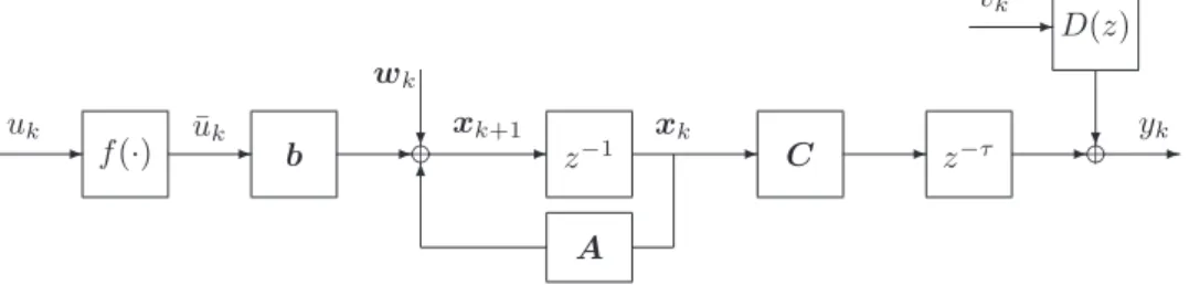
Consider the following Hammerstein nonlinear system as shown in Figure1, which is composed of a static nonlinear block followed by a linear dynamic subsystem. The linear subsystem is described by a state space model with moving average measurement noise. The time-delay is considered in the output block.
- f(·) - b -+d? -wk z−1 -A 6 C - z−τ -+d? -D(z) -vk uk u¯k xk+1 xk yk
Figure 1. The Hammerstein state space model with time-delay The Hammerstein state space model can be written as
xk+1=Axk+bu¯k+wk, (1) yk=cxk−τ+ nd X i=1 divk−i+vk, (2)
where yk is the measured output, u¯k is the output of the static nonlinear block, wk := [w1,k, w2,k,· · · , wn,k]T∈Rn and vk represent mutually independent process noise
and measurement noise with zero mean and variance Q and R, respectively. xk:= [x1,k, x2,k,· · ·, xn,k]T∈Rn is the system state vector.A∈Rn×n is the system parameter matrix, b∈Rnandc∈R1×nare the parameter vectors,
A:= −a1 1 0 · · · 0 −a2 0 1 ... .. . ... . .. 0 −an−1 0 · · · 0 1 −an 0 · · · 0 ∈Rn×n , b:= b1 b2 .. . bn−1 bn ∈Rn, c:= [1,0,0,· · ·,0]∈R1×n.
Assume that the output of the nonlinear block is a linear function of the known basis:
¯ uk =γ1f1(uk) +γ2f2(uk) +· · ·+γmfm(uk) = m X j=1 γjfj(uk). (3) whereγ′
isare the unknown coefficients andfi(uk)
′
sare the base functions. Let γ:= [γ1, γ2,· · · , γm]T∈Rm,
f(uk) := [f1(uk), f2(uk),· · ·, fm(uk)]∈R1
From (1), we have x1,k+1=−a1x1,k+x2,k+b1u¯k+w1,k, (4) x2,k+1=−a2x1,k+x3,k+b2u¯k+w2,k, .. . xi,k+1=−aix1,k+xi+1,k+biu¯k+wi,k, (5) .. . xn,k+1=−anx1,k+bnu¯k+wn,k. Multiplyingz−j−1
on both sides of (5) gives
xi,k−j=−aix1,k−j−1+xi+1,k−j−1+biu¯k−j−1+wi,k−j−1, j= 0,1,2,· · · , n. (6) Substituting (6) into (4), we have
x1,k+1=−a1x1,k−a2x1,k−1+x3,k−1+b2u¯k−1+b1u¯k+w2,k−1+w1,k
=−a1x1,k−a2x1,k−1−a3x1,k−2+x4,k−2+b3u¯k−2+b2u¯k−1+b1u¯k+w3,k−2
+w2,k−1+w1,k =−a1x1,k−a2x1,k−1− · · · −anx1,k−n+1+bnu¯k−n+1+· · ·+b2u¯k−1+b1u¯k +wn,k−n+1+· · ·+w1,k =− n X i=1 aix1,k−i+1+ n X i=1 bi m X j=1 γjfj(uk−i+1) + n X i=1 wi,k−i+1. (7)
Multiplying both sides of (7) byz−τ−1 gives x1,k−τ=− n X i=1 aix1,k−τ−i+ n X i=1 bi m X j=1 γjfj(uk−τ−i) + n X i=1 wi,k−τ−i. (8)
Substituting (8) into (2) gives yk=x1,k−τ+D(z)vk =− n X i=1 aix1,k−τ−i+ n X i=1 bi m X j=1 γjfj(uk−τ−i) + n X i=1 wi,k−τ−i+ nd X i=1 dndvk−i+vk. (9)
Note that the model in (9) contains the product of the parameter vectorsb and γ of the linear and nonlinear blocks, which increases the complexity of identification. Besides, any identification scheme cannot distinguish(b,γ)from(αb,γ/α)for some nonzero and finite constantα, because any pair(αb,¯uk/α)would produce identical input and output measurements. Therefore, in order to
get unique parameter estimates, one of the entries ofbandγhas to be fixed. Here, adopt the key term separation technique [34,35] and let the first element of the vectorbequal 1; i.e.,b1= 1. Then Equation (9) can be rewritten as
yk=− n X i=1 aix1,k−τ−i+ m X j=1 γjfj(uk−τ−i) + n X i=2 biu¯t−τ−i+ n X i=1 wi,k−τ−i+ nd X i=1 dndvk−i+vk. (10) Letn1= 2n+m+nd−1and define parameter vectors and information vectors as
ϑ:= [a1, a2,· · · , an,γT, b2, b3,· · ·, bn]T∈R2n+m −1 , d:= [d1, d2,· · ·, dnd] T∈ Rnd , ϕk:= [−x1,k−τ−1,−x1,k−τ−2,· · ·,−x1,k−τ−n,f(uk−τ−1),u¯k−τ−2,u¯k−τ−3,· · ·,u¯k−τ−n,φTk] T∈ Rn1,
φk:= [vk−1, vk−2,· · ·, vk−nd] T∈ Rnd, θ:= · ϑ d ¸ ∈Rn1.
Then Equation (10) can be written as yk =ϕTkθ+
n
X
i=1
wi,k−τ−i+vk.
Let ek:=Pni=1wi,k−τ−i+vk. Since both the process noise wk and measurement noise vk are
Gaussian white noises, and wk ∼N(0,Q), vk ∼N(0, R), then the output yk of the system in
Figure1can be expressed by the following pseudo-linear regressive form:
yk =ϕTkθ+ek. (11)
The objective of this paper is to derive identification algorithms to estimate the states and parametersai,bi,γi anddiand the time-delay (if it is unknown) for the Hammerstein state space
model by using the measured input-output data{uk, yk}.
For the model in (11), the number of the unknown parameters in the vectorθisn1:= 2n+m+
nd−1. In fact, there is another model which is called the over-parameterization model to deal with
the product term ofbandγ. For example, the method in [33] expresses the parameter vector as θ:= [a1, a2,· · ·, an, b1γ1, b2γ1,· · ·, bnγ1, b1γ2, b2γ2,· · · , bnγ2,· · ·,
b1γm, b2γm,· · ·, bnγm, d1, d2,· · · , dnd]
T∈Rn+nm+nd.
(12)
In that situation, the number of the unknown parameters in the vector θ is n2:=n+nm+nd.
Since bothnand mare positive integers, the difference between n1and n2 is∆n:=n2−n1=
nm−n−m+ 1>0. That means that the dimension of the unknown parameter vector in the over-parameterization method is larger than that in the key term separation based medthod. When the order of the state space model becomes higher or the polynomialf(ut)has more components, the
difference∆nwill become large. Thus the method of this paper requires lower computational load for realizing the parameter estimation algorithm.
3. THE KALMAN-FILTER BASED LEAST SQUARES ALGORITHMS WITH KNOWN TIME-DELAY
In process control industry, the phenomenon of time-delay often exists in the procedure of signal transmission. Based on the empirical knowledge, it is assumed that the time-delay is known. In this section, we derive the Kalman-filter based least squares algorithms to identify the Hammerstein dynamic system with known time-delay.
3.1. The state estimation algorithm
The Kalman filter can give the state estimates [36]. There are two steps in the Kalman filter, one is called the time update (or prediction), the other is called the measurement update (or modification). On the prediction step, the prior estimates of the state and its covariance are predicted; on the modification step, the newest measurement and prior estimates are combined together to modify the posterior estimates.
Because the parameter matrix/vectors are unknown, we need to use the estimated parameter vector
ˆ
θk:= [ˆa1,k,ˆa2,k,· · ·,ˆan,k,ˆγ1,k,γ2ˆ ,k,· · · ,γˆm,k,ˆb2,k,· · · ,ˆbn,k,d1ˆ,k,d2ˆ,k,· · · ,dˆnd,k]
to construct the estimatesAˆk andˆbk ofAandb, and use the estimated parameter matrixAˆk and
Kalman filter is used to generate the optimal state estimate. Considering the time delayτ in the output, we can use the following Kalman filter to obtain the state estimatexˆk+1[23]:
¯ xk+1= ˆAkxˆk+ ˆbku¯k, xˆ1=1n/p0 (13) ¯ Pk= ˆAkPkAˆ T k+Q, P1=In (14) Lk= ¯PkcT(cP¯kcT+R) −1 , (15) ˆ xk+1= ¯xk+1+Lk(yk+1+τ−cx¯k+1), (16) Pk+1= ¯Pk−LkcP¯k, (17) ˆ Ak= −a1ˆ ,k 1 0 · · · 0 −a2ˆ ,k 0 1 ... .. . ... . .. 0 −ˆan−1,k 0 · · · 0 1 −ˆan,k 0 · · · 0 , (18) ˆ bk= [1,ˆb2,k,ˆb3,k,· · ·,ˆbn,k]T, (19)
wherex¯k+1is a prior estimate of the statexk+1for given measurements up to and including timek;
ˆ
xk+1is a posterior estimate of the statexk+1for given measurements up to and including timek+ 1;
¯
Pk is the variance of the prior estimation error;Pk+1 is the variance of the posterior estimation error;Lkis the Kalman gain vector.
Another frequently used method for state estimation is to use the state observer [32] which can be used to get the approximate values of the system states. The drawback of the state observer is that it is generally suitable for deterministic systems. Thus this paper uses the parameter estimates based Kalman filter for generating the state estimates in the stochastic framework.
3.2. The iterative parameter estimation algorithm
Opt a set of data fromj=ktoj=k+L−1(Ldenotes the data length) and define the stacked output vectorYk,Land stacked information matrixΦk,Las
Yk,L:= yk yk+1 .. . yk+L−1 ∈RL; Φk,L:= ϕT k ϕT k+1 .. . ϕT k+L−1 ∈RL×n1 .
According to (11), we define a criterion function J1(θ) =kYk,L−Φk,Lθk2.
Lets= 1,2,3,· · · be an iterative variable andθˆskbe the estimate ofθat iterations. Minimizing the
criterion functionJ1(θ)and letting the derivative ofJ1(θ)with respect toθbe zero gives ∂J1(θ) ∂θ ¯ ¯ ¯ ¯θ= ˆθs k =−2ΦT k,L[Yk,L−Φk,Lˆθ s k] =0.
Then we can obtain the least squares estimate of the parameter vectorθ:
ˆ
θsk= [ΦT
k,LΦk,L]
−1ΦT
k,LYk,L. (20)
But we cannot obtain the estimateθˆskdirectly from (20), because the information vectorϕkinΦk,L
contains the unknown state variablex1,k−τ−i, the unknown outputu¯k−iof the nonlinear block and
the unknown noise termsvk−j. The scheme here is to replacex1,k−τ−i,u¯k−iandvk−j inϕk with
their corresponding estimatesxˆs−1 1,k−τ−i,uˆ¯
s−1
k−iandvˆ s−1
k−j at iterations−1and define ˆ ϕsk= [−xˆ s−1 1,k−τ−1,−xˆ s−1 1,k−τ−2,· · ·,−xˆ s−1 1,k−τ−n,f(uk−τ−1),uˆ¯s −1 k−τ−2,· · ·,uˆ¯ s−1 k−τ−n,vˆ s−1 k−1,
ˆ vs−1 k−2,· · ·,vˆ s−1 k−nd] T.
Replacing the unknown coefficientγjin (3) with its estimateˆγj,ks gives ˆ ¯ us k = ˆγ s 1,kf1(uk) + ˆγs2,kf2(uk) +· · ·+ ˆγm,ks fm(uk). From (2), we have vk=yk−cxk−τ−dTφk. (21)
Replace xk−τ, φk and din (21) with their estimates xˆ s k−τ, φˆ
s k and dˆ
s
k, the estimate ˆvks can be
computed by ˆ vs k=yk−cxˆsk−τ−(ˆd s k) Tˆ φsk. Define ˆ Φs k,L:= [ ˆϕ s k,ϕˆ s k+1,· · ·,ϕˆ s k+L−1] T∈ RL×n1.
Replacing the information matrixΦk,Lin (20) with its estimateΦˆs
k,Land using the Kalman filter to
obtain the estimates of the unknown states, we can get the Kalman-filter based least squares iterative (KF-LSI) algorithm for estimating the parameters and states of the Hammerstein state space models:
ˆ θsk= [( ˆΦ s k,L)TΦˆ s k,L] −1 ( ˆΦs k,L)TYk,L, (22) Yk,L= [yk, yk+1,· · ·, yk+L−1]T, (23) ˆ Φs k,L= [ ˆϕ s k,ϕˆ s k+1,· · ·ϕˆ s k+L−1] T, (24) ˆ ϕsk= [−xˆ s−1 1,k−τ−1,−xˆ s−1 1,k−τ−2,· · · ,−xˆ s−1 1,k−τ−n,f(uk−τ−1),uˆ¯s −1 k−τ−2,· · · ,uˆ¯ s−1 k−τ−n, ˆ vs−1 k−1,· · · ,vˆ s−1 k−nd] T, (25) ˆ¯ us k= ˆγ s 1,kf1(uk) + ˆγ2s,kf2(uk) +· · ·+ ˆγm,ks fm(uk), (26) ˆ vs k=yk−cxˆsk−τ−(ˆd s k)Tφˆ s k, (27) ˆ θsk= [ˆas1,k,ˆas2,k,· · ·,ˆasn,k,ˆγs1,k,γˆ2s,k,· · · ,γˆm,ks ,ˆbs2,k,· · · ,ˆbn,ks ,dˆs1,k,· · ·,dˆsnd,k] T, (28) ˆ Ask= −aˆs 1,k 1 0 · · · 0 −aˆs 2,k 0 1 ... .. . ... . .. 0 −ˆas n−1,k 0 · · · 0 1 −ˆas n,k 0 · · · 0 , (29) ˆ bsk= [1,ˆb s 2,k,ˆb s 3,k,· · ·,ˆb s n,k]T, (30) ¯ xsk+1= ˆA s kxˆ s k+ ˆb s ku¯k, xˆs1=1n/p0, (31) ¯ Pk= ˆA s kPk( ˆA s k)T+Q, P1=In, (32) Lk= ¯PkcT(cP¯kcT+R) −1 , (33) ˆ xsk+1= ¯x s k+1+Lk(yk+1+τ−cx¯sk+1), (34) Pk+1= ¯Pk−LkcP¯k. (35)
Remark 1The iterative algorithm is implemented off-line, it repeatedly uses a batch of observed
data and can get good parameter estimates after only several iterations [37,38,39,40]. In the LSI algorithm, the measured input-output data should be collected in advance.
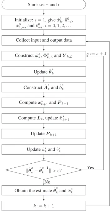
The flowchart of computing the parameter estimatesˆθsk and the state estimatexˆ s
k by the KF-LSI
Start: setτandǫ ¶ µ ³ ´ ? Initialize:s= 1, givexˆ1k,uˆ¯0−i, ˆ x0 1,−iandˆv 0 −i,i= 0,1,2, . . . ?
Collect input and output data ? Constructϕˆsk,Φ s k,LandYk,L ? Updateˆθsk ? ConstructAˆskandˆb s k ? Computex¯s k+1andP¯k+1 ? ComputeLk, updatexˆsk+1 ? UpdatePk+1 ? Updateuˆ¯s kandvˆ s k ? » » » » » » » » » XXXXXXXXX X X X X X X X X X »»»»»» »»» kθˆsk−θˆ s−1 k k> ε? No Yes ¾s:=s+ 1 ?
Obtain the estimateθˆskandxˆ s k
?
k:=k+ 1
¾
Figure 2. The flowchart of the KF-LSI algorithm for computingˆθs
k,xˆsk
3.3. The recursive parameter estimation algorithm
Unlike the LSI algorithm, the RLS algorithm may be carried out on-line. By defining a covariance matrix, the RLS algorithm uses the input and output data to update the parameter estimates at each step. In this section, a Kalman filter based RLS algorithm is derived.
Similarly, according to (11), define a quadratic criterion function J2(θ) = k X j=1 [y(j)−ϕT jθ] 2 .
Minimizing J2(θ) using the least squares principle, letting the partial derivative of J2(θ) with respect toθbe zero, we can obtain
ˆ
θk= ˆθk−1+L1,k[yk−ϕTkθˆk−1], (36)
L1,k=P1,k−1ϕk[1 +ϕTkP1,k−1ϕk] −1
, (37)
P1,k= [I−L1,kϕTk]P1,k−1. (38)
Because the information vector ϕk contains the unmeasurable state variable x1,k−τ−i, unknown
output of nonlinear blocku¯k−i and the unknown noisevk−j, the algorithm in (36)–(38) cannot be
implemented. Here we replacex1,k−τ−i,u¯k−i andvk−j inϕk with their corresponding estimates ˆ
x1,k−τ−i,uˆ¯k−iandvˆk−jat timekand define ˆ
ϕk:= [−x1ˆ ,k−τ−1,−x1ˆ ,k−τ−2,· · · ,−x1ˆ ,k−τ−n,f(uk−τ−1),uˆ¯k−τ−2,· · · ,uˆ¯k−τ−n, ˆ
vk−1,· · · ,vˆk−nd]
T∈Rn1.
Replacing the unknown coefficientγjin (3) with its estimateˆγj,kgives ˆ
¯
uk = ˆγ1,kf1(uk) + ˆγ2,kf2(uk) +· · ·+ ˆγm,kfm(uk). (39)
Replacing xk−τ,φk and din (21) with their estimates xˆk−τ,φˆk and ˆdk, the estimatevˆk can be
computed by
ˆ
vk=yk−cxˆk−τ−dˆ T
kφˆk. (40)
Then we can summarize the following RLS algorithm for estimating the parameter vectorθas
ˆ θk= ˆθk−1+L1,k[yk−ϕˆTkθˆk−1], (41) L1,k=P1,k−1ϕˆk[1 + ˆϕ T kP1,k−1ϕˆk] −1 , (42) P1,k= [In1−L1,kϕTk]P1,k−1, P1,0=p0In1, (43) ˆ ϕk= [−x1ˆ ,k−τ−1,−x1ˆ ,k−τ−2,· · ·,−x1ˆ ,k−τ−n,f(uk−τ−1),uˆ¯k−τ−2,· · ·,uˆ¯k−τ−n, ˆ vk−1,· · ·,ˆvt−nd] T, (44) ˆ θk= [ˆa1,k,ˆa2,k,· · · ,aˆn,k,γ1ˆ ,k,γ2ˆ ,k,· · ·,ˆγm,k,ˆb2,k,· · · ,ˆbn,k,d1ˆ,k,· · · ,dˆnd,k] T, (45) ˆ¯ uk= ˆγ1,kf1(uk) + ˆγ2,kf2(uk) +· · ·+ ˆγm,kfm(uk), (46) ˆ vk=yk−cxˆk−τ−dˆ T kφˆk. (47)
For the unknown statex1,k, we also use the Kalmam filter algorithm to generate its estimatexˆ1,k.
Combining Equations (41)–(47) and (13)–(19), we can get the Kalman-filter based recursive least squares (KF-RLS) algorithm for identifying the Hammerstein state space systems.
To initialize the KF-RLS algorithm, the initial value θˆ0 and xˆ1 is generally taken to be a real vector, e.g., θˆ0=1n1/p0 and xˆ1=1n/p0 with p0 being normally a large positive
number (e.g.,p0= 106
). Letx1ˆ ,−i= 1/p0,uˆ¯−i= 1/p0andˆv−j= 1/p0 fori= 0,1,2,· · ·, n, j= 0,1,2,· · ·, nd−1. The initial values of the covariance matrixes are set asP1,0=p0In1,P1=In.
4. THE REDUNDANT RELS ALGORITHM FOR HAMMERSTEIN SYSTEMS WITH UNKNOWN TIME-DELAY
Although we can predict the time-delay based on the empirical data in some special cases, there are many uncertain varying elements which bring the unknown time-delay in the actual systems. Besides identifying the system parameters, we also need to get the estimate of the time-delay based on the observed data.
Reconsidering (11), if we extend the information vectorϕkand supplement the lost terms which
are omitted because of the time-delay. The information vectorϕ¯kis redefined as
¯ ϕk:= [−x1,k−1,−x1,k−2,· · ·,−x1,k−τ,−x1,k−τ−1,−x1,k−τ−2,· · ·,−x1,k−τ−n,f(uk−τ−1), ¯ uk−τ−2,· · ·,u¯k−τ−n, vk−1, vk−2,· · · , vk−nd] T∈ Rn1+τ.
At the same time, the parameter vectorθis extended as the following form:
¯
θ:= [a01, a02,· · ·, a0τ, a1, a2,· · · , an, γ1, γ2,· · · , γm, b2, b3,· · · , bn, d1, d2,· · ·, dnd]
T∈
The dimension of θ¯ is larger than the dimension of the original parameter vector θ because of the redundant parameters{a01, a02,· · · , a0τ}. In fact, the true values of the redundant parameters
should be zeros to guarantee the model structure unchanged. So the number of the redundant parameters is the value of the time-delay τ. Once the estimates of the redundant parameters lie in a given confidence interval, we can assume them as zero. So the number of the continuous approximate zero elements in the front part of the estimate ofθ¯is the estimate of the time-delayτ. Then our objective is how to obtain the estimateˆ¯θkof¯θk.
Rewrite the model in (11) as
yk = ¯ϕTk¯θ+ek. (48)
Define a quadratic criterion function J3(¯θ) := k X j=1 [y(j)−ϕ¯T j¯θ] 2 .
MinimizingJ3(¯θ)and using the least squares principle, we can get the following relations:
ˆ ¯θk= ˆ¯θk−1+L2,k[yk−ϕ¯Tkˆ¯θk−1], (49) L2,k=P2,k−1ϕ¯k[1 + ¯ϕ T kP2,k−1ϕ¯k] −1 , (50) P2,k= [I−L2,kϕ¯Tk]P2,k−1. (51)
Similarly, the information vectorϕ¯k contains the unknownx1,k−i,u¯k−iandvk−j, the algorithm in
(49)–(51) cannot be implemented. Replacex1,k−i,u¯k−i andvk−j inϕ¯k with their corresponding
estimatesx1ˆ ,k−i,uˆ¯k−iandˆvk−jat timekand define ˆ¯ ϕk:= [−x1ˆ ,k−1,−x1ˆ ,k−2,· · ·,−x1ˆ ,k−τ,−x1ˆ ,k−τ−1,−x1ˆ ,k−τ−2,· · ·,−ˆx1,k−τ−n,f(uk−τ−1), ˆ¯ uk−τ−2,· · ·,uˆ¯k−τ−n,vˆk−1,· · · ,ˆvk−nd] T∈ Rn1+τ.
Replacingϕ¯kin (49)–(51) with its estimateϕˆ¯k, we can summarize the following recursive extended
least squares (RELS) algorithm for estimating¯θ:
ˆ¯ θk= ˆ¯θk−1+L2,k[yk−ϕˆ¯Tkˆ¯θk−1], (52) L2,k=P2,k−1ϕˆ¯k[1 + ˆ¯ϕTkP2,k−1ϕˆ¯k] −1 , (53) P2,k= [I−L2,kϕˆ¯Tk]P2,k−1, (54) ˆ¯ ϕk= [−x1ˆ ,k−1,−x1ˆ ,k−2,· · ·,−x1ˆ ,k−τ,−x1ˆ ,k−τ−1,−x1ˆ ,k−τ−2,· · ·,−ˆx1,k−τ−n,· · · , f(uk−τ−1),uˆ¯k−τ−2,uˆ¯k−τ−n,ˆvk−1,· · · ,vˆk−nd] T, (55) ˆ¯ θk= [ˆa01,k,a02ˆ ,k,· · ·,ˆa0τ,k,a1ˆ ,k,ˆa2,k,· · · ,ˆan,k,γ1ˆ ,k,· · · ,γˆm,k,ˆb2,k,· · · ,ˆbn,k,d1ˆ,k,· · ·,dˆnd,k] T, (56) ˆ¯ uk= ˆγ1,kf1(uk) + ˆγ2,kf2(uk) +· · ·+ ˆγm,kfm(uk), (57) ˆ vk=yk−cxˆk−τ−dˆ T kφˆk. (58)
Combining (52)–(58) and (13)–(19), the Kalman-filter based recursive extended least squares (KF-RELS) algorithm for estimatingθ¯is obtained. Then the value of the time-delayτ can be evaluated by counting how many elements which are close to zero in the front part ofˆ¯θk.
The steps for computing the state and parameter estimates xˆk and ˆ¯θk under the KF-RELS
algorithm with the increasing ofkare as follows.
1. To initialize. Letk= 1, the initial valueˆ¯θ0 and xˆ1 is generally taken to be a real vector, e.g.,θˆ0=1n1+τ/p0 and xˆ1=1n/p0. Letx1ˆ ,−i= 1/p0,uˆ¯−i= 1/p0 and ˆv−j = 1/p0 (i= 0,1,2,· · ·, j= 0,1,2,· · · , nd−1). The initial values of the covariance matrixes are set as:
¯
P0=p0In1+τ,P1=In. Give a small positiveε.
2. Collect the input-output data, construct the information vectorϕˆkby (55). 3. Compute the gain vectorL2,kand the covariance matrixP2,kby (53) and (54). 4. Update the parameter estimatesˆ¯θkby (52).
5. Construct the matrixAˆkby (18), and the vectorˆbk by (19).
6. Compute the prior estimatex¯k+1and the covariance matrixP¯kby (13) and (14).
7. Compute the Kalman gainLk by (15), update the posterior state estimatexˆk+1 by (16) and the posterior covariance matrixPk+1by (17).
8. Update the estimatesuˆ¯k andˆvkby (57) and (58). 9. Evaluate the relative error of parameter estimates, if
δ=kˆ¯θk−ˆ¯θk−1k6ε
for some pre-set smallε, then terminate this procedure and obtain the parameter estimateˆ¯θk
and the state estimatexˆk+1; otherwise, increasekby1and go to Step2.
5. EXAMPLE
Example 1: Consider the following Hammerstein system with state space model:
xk+1=Axk+bu¯k+wk,
yk=cxt−τ−0.30vk−1+vk, ¯
uk=γ1uk+γ2u2k+γ3u
3 k, A= · −0.50 1 −0.26 0 ¸ , b= · 1 1.50 ¸ , c= [1, 0], γ= [0.25,0.60,0.76].
In simulation, the input {uk} is taken as a persistent excitation sequence with zero mean and unit variance, and {wk}, {vk} as uncorrelated noise sequences with zero mean and variances Q:= · σ2 w 0 0 σ2 w ¸ and R:=σ2
v, respectively. The output time-delay τ= 2. Using the KF-LSI
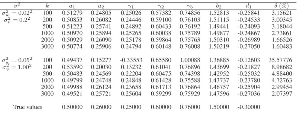
algorithm and KF-RLS algorithm to estimate the parameters of this model, the parameter estimates and their estimation errorsδ:=kθˆk−θk/kθkwith different noise variances are shown in TablesI– II. In the KF-LSI algorithm, the data lengthL= 1000.
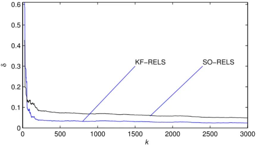
To show the advantage of Kalman filter in obtaining the estimates of unknown states, the state observer (SO) is also used to get the estimates of the unknown system states. Combining the SO with the LSI and RLS algorithm to get the SO-LSI estimates and the SO-RLS estimates. The estimation errors versussorkare plotted in Figure3and Figure4.
From TablesI–IIIand Figures3–4, we can draw the following conclusions.
1. It is clear see that the estimation errors δ are becoming smaller (in general) as s or k increasing. This indicates that the proposed KF-LSI and KF-RLS algorithms are effective for Hammerstein state space systems.
2. A smaller noise variance leads to smaller parameter estimation errors under the same data length in the KF-LSI and KF-RLS algorithm.
3. The proposed KF-LSI and KF-RLS algorithm have better performances on estimation accuracy than the SO-LSI and SO-RLS estimation algorithm.
For comparison, we use the state observer based hierarchical stochastic gradient (SO-HSG) algorithm and the hierarchical multi-innovation stochastic gradient (SO-HMISG) algorithm in [31] and the state observer based hierarchical least squares (SO-HLS) algorithm in [32] to identify this model. In order to acquire the unique estimate, they assume that the norm of the coefficient vector γis unity and the first coefficient is positive, i.e.,kγk2= 1
(RMSE), RMSE = v u u t L X j=1 [yj−yˆj]2/L
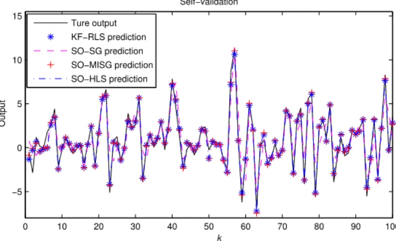
is employed to reflect the errors between the predicted values and true values. Using the Monte Carlo simulations with 100 set of noise realizations, the RMSE and its bias of the five different algorithms are summarized in Table III. The results of self-validation and cross-validation of the discussed different algorithms are shown in Figures5and6.
From Figures5–6and TableIII, we can see that 1) the KF-LSI algorithm has the smallest RMSE in the self-validation and cross validation, 2) the KF-RLS algorithm has better performances in prediction than other algorithms, 3) the RMSE of the SO-HSG algorithm is obvious larger than those of other four algorithms, by extending the length of the innovation, the SO-HMISG algorithm can enhance the accuracy of parameter estimation.
Table I. The KF-LSI parameter estimates and errors versuss
σ2 s a1 a2 γ1 γ2 γ3 b2 d1 δ(%) σ2 w= 0.02 2 1 0.50024 0.26313 0.24944 0.59815 0.75849 1.49801 -0.00523 15.41463 σ2 v= 0.2 2 2 0.51093 0.26052 0.24857 0.59917 0.75988 1.50482 -0.25617 2.37727 5 0.50822 0.26122 0.24882 0.59880 0.75964 1.50185 -0.29186 0.62240 10 0.50822 0.26121 0.24882 0.59875 0.75964 1.50184 -0.29185 0.62308 15 0.50822 0.26121 0.24882 0.59876 0.75964 1.50184 -0.29185 0.62308 σ2 w= 0.05 2 1 0.50088 0.27553 0.24811 0.59074 0.75278 1.49015 -0.02357 14.49929 σ2 v= 1.00 2 2 0.50629 0.28097 0.24377 0.58957 0.75995 1.50340 -0.27305 1.93178 5 0.50402 0.27903 0.24510 0.59069 0.75864 1.49624 -0.29440 1.21077 10 0.50402 0.27897 0.24509 0.59063 0.75863 1.49619 -0.29440 1.21021 15 0.50402 0.27897 0.24509 0.59064 0.75863 1.49619 -0.29440 1.21016 True values 0.50000 0.26000 0.25000 0.60000 0.76000 1.50000 -0.30000
Table II. The KF-RLS parameter estimates and errors versusk
σ2 k a1 a2 γ1 γ2 γ3 b2 d1 δ(%) σ2 w= 0.02 2 100 0.51279 0.24805 0.25026 0.57382 0.74856 1.52813 -0.25841 3.15621 σ2 v= 0.2 2 200 0.50853 0.26082 0.24446 0.59100 0.76103 1.51115 -0.24533 3.00345 500 0.51223 0.25741 0.24892 0.60433 0.76192 1.49441 -0.24093 3.18044 1000 0.50970 0.25894 0.25265 0.60038 0.75789 1.49877 -0.24867 2.73861 2000 0.50929 0.26090 0.25178 0.59864 0.75763 1.50310 -0.26989 1.66526 3000 0.50774 0.25906 0.24794 0.60148 0.76008 1.50219 -0.27050 1.60483 σ2 w= 0.05 2 100 0.49437 0.15277 -0.33553 0.65580 1.00088 1.36885 -0.12603 35.57776 σ2 v= 1.00 2 200 0.53590 0.20030 0.13232 0.61041 0.76896 1.43699 -0.21827 8.98682 500 0.50483 0.24569 0.22204 0.60475 0.74398 1.42952 -0.25032 4.88400 1000 0.49799 0.24748 0.24848 0.61428 0.75588 1.43737 -0.23780 4.72763 2000 0.49988 0.26124 0.23658 0.61713 0.76864 1.46757 -0.25904 2.99454 3000 0.49521 0.25721 0.25604 0.59299 0.75929 1.47596 -0.27036 2.07397 True values 0.50000 0.26000 0.25000 0.60000 0.76000 1.50000 -0.30000
Example 2: Consider a following Hammerstein system with unknown time-delay:
xk+1=Axk+bu¯k+wk, yk=cxt−τ−0.18vk−1+vk, ¯ uk=γ1sin(uk) +γ2cos(uk), A= · −0.45 1 −0.30 0 ¸ , b= · 1 1.50 ¸ , c= [1, 0], γ= [1.20, −0.32].
Table III. The RMSE and its bias of different algorithms based on 100 Monte Carlo runs (σw2 = 0.022,
σv2= 0.202)
RMSE
Algorithm Self-validation Cross-validation
KF-LSI 0.22374±0.00706 0.22602±0.02726 KF-RLS 0.23852±0.00708 0.26681±0.02815 SO-HSG 1.28185±0.24508 1.12947±0.13251 SO-HMISG(p=6) 0.30017±0.29869 0.35248±0.10866 SO-HLS 0.27849±0.10688 0.36280±0.05659 0 5 10 15 0 0.02 0.04 0.06 0.08 0.1 0.12 0.14 0.16 KF−LSI SO−LSI s δ
Figure 3. The SO-LSI and KF-LSI estimation errorsδversuss(σ2w= 0.022,σv2= 0.202)
0 500 1000 1500 2000 2500 3000 0 0.1 0.2 0.3 0.4 0.5 0.6 SO−RELS KF−RELS k δ
Figure 4. The SO-RLS and KF-RLS estimation errorsδversusk(σw2 = 0.022,σ2v= 0.202)
Take the same simulation conditions as those in Example 1 and let σ2
w= 0.02 2 and σ2 v= 0.20 2 . Using the KF-RELS algorithm to estimate the parameters, states and time-delay of this system, the parameter estimates and their estimation errors are shown in TableIV. Give a confidence interval
[−0.005,0.005]for the redundant parameters. Checking the last second line in TableIV, we can find there are two elements which can be assumed as zero. So the time-delayτequals2.
As a comparison, use the state observer to estimate the unknown system states again. Combining it with the RELS algorithm to get the SO-RELS estimates. The parameter estimates and their
0 10 20 30 40 50 60 70 80 90 100 −5 0 5 10 15 Self−validation k Output Ture output KF−RLS prediction SO−SG prediction SO−MISG prediction SO−HLS prediction
Figure 5. A section of the self-validation of different algorithms (σw2 = 0.022,σv2= 0.202)
3000 3010 3020 3030 3040 3050 3060 3070 3080 3090 3100 −5 0 5 10 Cross−validation k Output Ture output KF−RLS prediction SO−SG prediction SO−MISG prediction SO−HLS prediction
Figure 6. A section of the cross-validation of different algorithms (σw2 = 0.022,σ2v= 0.202)
estimation errors are also shown in TableIV. From TableIV, we can see that the KF-RELS algorithm generates better estimates than the SO-RELS algorithm.
For model validation, a different dataset (Le= 200 samples from t= 3001 to 3200) and the
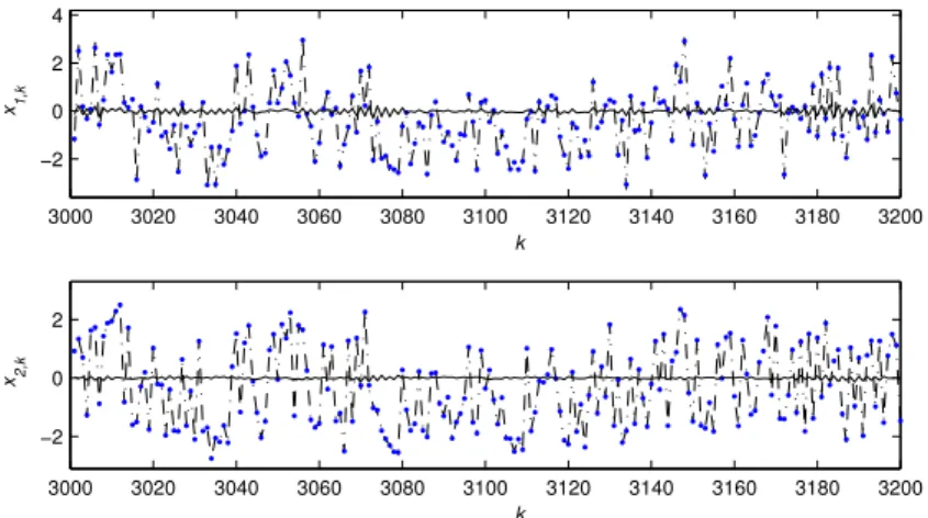
estimated model obtained by the KF-RELS algorithm are used. The predicted output and the true output under the KF-RELS algorithm are plotted in Figure7. The true states and the estimated states are compared in Figure8. From Figures7–8, we can draw the following conclusions.
1. The model outputs can fit the true outputs well, the KF-RELS algorithm can capture the dynamic system well.
2. The estimated states are very close to the true states, the parameter estimates based Kalman filter can generate highly accurate state estimates.
6. CONCLUSIONS
A Kalman filter based least squares iterative algorithm and recursive least squares algorithm are developed for Hammerstein systems with dynamic state space model. The process noise is assumed to be white noise, the measurement noise is fitted by the moving average noise. For the unknown Copyright c°2016 John Wiley & Sons, Ltd. Int. J. Adapt. Control Signal Process.(2016)
Table IV. The SO-RELS and KF-RELS parameter estimates and errors versusk Algorithm k a01 a02 a1 a2 γ1 γ2 b2 d1 δ(%) SO-RELS 100 0.02795 0.18176 0.48168 -0.20607 1.45273 -0.47187 1.51377 -0.27369 16.61618 200 0.01253 0.15293 0.47055 -0.23135 1.43085 -0.41217 1.45089 -0.27925 13.90675 500 0.00365 0.12384 0.47863 -0.25194 1.39700 -0.38491 1.40655 -0.28999 12.30822 1000 -0.00232 0.10862 0.48803 -0.26634 1.36120 -0.36924 1.41128 -0.29300 10.67716 2000 0.00346 0.08652 0.47877 -0.27692 1.33084 -0.35337 1.39472 -0.26988 8.79811 3000 0.00633 0.07844 0.48158 -0.28087 1.32018 -0.35446 1.40312 -0.25708 7.95681 KF-RELS 100 0.03284 0.03973 0.49893 -0.20725 1.21083 -0.45434 1.30588 -0.32613 13.40018 200 0.02832 0.04168 0.49727 -0.27377 1.26652 -0.37328 1.39482 -0.23716 6.44682 500 0.00907 0.04078 0.49278 -0.29927 1.27048 -0.34336 1.42444 -0.20737 4.69370 1000 -0.00230 0.02711 0.49244 -0.30931 1.23701 -0.32881 1.43377 -0.19160 3.06655 2000 0.00198 0.00730 0.48081 -0.31664 1.21497 -0.31732 1.41960 -0.17097 2.49090 3000 0.00442 -0.00050 0.48446 -0.31938 1.20665 -0.31978 1.42942 -0.16938 2.32384 True values 0.00000 0.00000 0.45000 -0.30000 1.20000 -0.32000 1.50000 -0.18000 3000 3020 3040 3060 3080 3100 3120 3140 3160 3180 3200 −4 −3 −2 −1 0 1 2 3 4 5 k Output True output y(t) Predicted output
Figure 7. The KF-RELS predicted output and true output versusk
3000 3020 3040 3060 3080 3100 3120 3140 3160 3180 3200 −2 0 2 4 k x1,k 3000 3020 3040 3060 3080 3100 3120 3140 3160 3180 3200 −2 0 2 k x2,k
Solid line: the estimation error; dashed: the truexk; dots: the estimatedxˆk Figure 8. The statexkand estimated estimatexˆkversusk
time-delay in the output block, a Kalman filter based recursive extended least squares algorithm is derived. Based on the proposed algorithms, the combined state and parameter estimation are
obtained. The proposed algorithms can be extended to other system identification models, e.g., the linear state space models, and Wiener models [41,42] and Hammerstein-Wiener systems [43,44] or applied to nonlinear systems [45,46] and other fields [47,48,49].
7. ACKNOWLEDGEMENTS
This work was supported by the National Natural Science Foundation of China (No. 61273194), the Graduate Education Innovation Program of Jiangsu Province (No. KYLX16 0780) and the 111 Project (B12018).
REFERENCES
1. van der Veen G, van Wingerden JW, Verhaegen M. Global identification of wind turbines using a Hammerstein identification method.IEEE Transactions on Control Systems Technology2013;21(4): 1471–1478.
2. Wang J, Zhang Q. Detection of asymmetric control valve stiction from oscillatory data using an extended Hammerstein system identification method.Journal of Process Control2014;24(1): 1–12.
3. Kim J, Konstantinou K. Digital predistortion of wideband signals based on power amplifier model with memory.
IEE Electronics Letters2001;37: 1417–1418.
4. Zhang LM, Hua CC, Guan XP. Structure and parameter identification for Bayesian Hammerstein system.Nonlinear Dynamics2015;79(3): 1847–1861.
5. Chen J, Wang XP. Identification of Hammerstein systems with continuous nonlinearity.Information Processing Letters2015;115(11): 822–827.
6. Zhao S, Huang B, Liu F. Minimum variance unbiased FIR filter for discrete time-variant systems.Automatica2015; 53(3): 355-361.
7. Zhao S, Shmaliy YS, Liu F. Fast Kalman-like optimal unbiased FIR filtering with applications.IEEE Transactions on Signal Processing2016;64(9): 2284-2297.
8. Wang DQ, Zhang W. Improved least squares identification algorithm for multivariable Hammerstein systems.
Journal of the Franklin Institute2015;352(11): 5292–5307.
9. Chen HB, Xiao YS, Ding F. Hierarchical gradient parameter estimation algorithm for Hammerstein nonlinear systems using the key term separation principle. Applied Mathematics and Computation2014;247: 1202–1210.
10. Liu Y, Bai EW. Iterative identification of Hammerstein systems.Automatica2007;43(2): 346–354.
11. Wang XX, Liang Y, Pan Q, Zhao CH, Yang F. Nonlinear gaussian smoothers with colored measurement noise.IEEE Transactions on Automatic Control2015;60(3): 870–876.
12. Roopa S, Narasimhan SV, Babloo B. Steiglitz–McBride adaptive notch filter based on a variable-step-size LMS algorithm and its application to active noise control.International Journal of Adaptive Control and Signal Processing
2016;30(1): 16–30.
13. Xu L, Ding F. Recursive least squares and multi-innovation stochastic gradient parameter estimation methods for signal modeling. Circuits, Systems and Signal Processing2017;36. doi: 10.1007/s00034-016-0378-4
14. Huang J, Shi Y, Huang HN, Li Z. l-2–l-infinity filtering for multirate nonlinear sampled-data systems using T-S fuzzy models.Digital Signal Processing2013;23(1): 418–426.
15. Wang YJ, Ding F. Novel data filtering based parameter identification for multiple-input multiple-output systems using the auxiliary model.Automatica2016;71: 308–313.
16. Wang YJ, Ding F. The filtering based iterative identification for multivariable systems.IET Control Theory and Applications2016;10(8): 894–902.
17. Wang YJ, Ding F. The auxiliary model based hierarchical gradient algorithms and convergence analysis using the filtering technique.Signal Processing2016;128: 212–221.
18. Hu YB, Liu BL, Zhou Q, Yang C. Recursive extended least squares parameter estimation for Wiener nonlinear systems with moving average noises.Circuits, Systems, and Signal Processing2014;33(2): 655–664.
19. Li JH. Parameter estimation for Hammerstein CARARMA systems based on the Newton iteration. Applied Mathematics Letters2013;26(1): 91–96.
20. Ding J, Lin JX. Modified subspace identification for periodically non-uniformly sampled systems by using the lifting technique.Circuits, Systems, and Signal Processing2014;33(5): 1439–1449.
21. Uzinski JC, Paiva HM, Duarte MA, Galv˜ao RK, Villarreal F. A state-space description for perfect-reconstruction wavelet FIR filter banks with special orthonormal basis functions. Journal of Computational and Applied Mathematics2015;290: 290–297.
22. Yan LP, Jiang L, Xia YQ, Fu MY. State estimation and data fusion for multirate sensor networks.International Journal of Adaptive Control and Signal Processing2016;30(1): 3–15.
23. Ding F, Liu XM, Ma XY. Kalman state filtering based least squares iterative parameter estimation for observer canonical state space systems using decomposition.Journal of Computational and Applied Mathematics2016;301: 135–143.
24. Zhang H, Shi Y, Wang JM. On energy-to-peak filtering for nonuniformly sampled nonlinear systems: a Markovian jump system approach.IEEE Transactions on Fuzzy Systems2014;22(1): 212–222.
25. Zhao S, Huang B, Liu F. Linear optimal unbiased filter for time-variant systems without apriori information on initial condition.IEEE Transactions on Automatic Control2016; doi: 10.1109/TAC.2016.2557999.
26. Ding F, Liu XM, Gu Y. An auxiliary model based least squares algorithm for a dual-rate state space system with time-delay using the data filtering.Journal of the Franklin Institute2016;353(2): 398–408.
27. Chen L, Han LL, Huang B, Liu F. Parameter estimation for a dual-rate system with time delay.ISA transactions
2014;53(5): 1368–1376.
28. Xie L, Yang HZ. Gradient based iterative identification for nonuniform sampling output error systems,Journal of Vibration and Control2011;17(3): 471–478.
29. Sch¨on TB, Wills A, Ninness B. System identification of nonlinear state-space models.Automatica2011;47(1): 39–49.
30. Deng J, Huang B. Identification of nonlinear parameter varying systems with missing output data.AIChE Journal
2012;58(11): 3454–3467.
31. Wang XH, Ding F. Recursive parameter and state estimation for an input nonlinear state space system using the hierarchical identification principle.Signal Processing2015;117: 208–218.
32. Wang DQ, Ding F, Liu XM. Least squares algorithm for an input nonlinear system with a dynamic subspace state space model.Nonlinear Dynamics2014;75(1-2): 49–61.
33. Wang XH, Ding F. Joint estimation of states and parameters for an input nonlinear state-space system with colored noise using the filtering technique.Circuits, Systems, and Signal Processing2015;35(2): 481–500.
34. V¨or¨os J. Modeling and parameter identification of systems with multi-segment piecewise-linear characteristics.IEEE Transactions on Automatic Control2002;47(1): 184–188.
35. V¨or¨os J. Recursive identification of Hammerstein systems with discontinuous nonlinearities containing dead-zones.
IEEE Transactions on Automatic Control2003;48(12): 2203–2206.
36. Pan J, Yang XH, Cai HF, Mu BX. Image noise smoothing using a modified Kalman filter.Neurocomputing2016; 173: 1625–1629.
37. Xu L. The damping iterative parameter identification method for dynamical systems based on the sine signal measurement, Signal Processing 120 (2016) 660-667.
38. Xu L. Application of the Newton iteration algorithm to the parameter estimation for dynamical systems.Journal of Computational and Applied Mathematics2015;288: 33–43.
39. Xu L, Chen L, Xiong WL. Parameter estimation and controller design for dynamic systems from the step responses based on the Newton iteration.Nonlinear Dynamics2015;79(3): 2155-2163.
40. Xu L. A proportional differential control method for a time-delay system using the Taylor expansion approximation.
Applied Mathematics and Computation2014;236: 391–399.
41. Ding F, Liu XM, Liu MM. The recursive least squares identification algorithm for a class of Wiener nonlinear systems.Journal of the Franklin Institute2016;353(7): 1518–1526.
42. Ding F, Wang XH, Chen QJ, Xiao YS. Recursive least squares parameter estimation for a class of output nonlinear systems based on the model decomposition.Circuits, Systems and Signal Processing2016;35(9): 3323–3338.
43. Wang YJ, Ding F. Recursive least squares algorithm and gradient algorithm for Hammerstein-Wiener systems using the data filtering.Nonlinear Dynamics2016;84(2): 1045–1053.
44. Wang YJ, Ding F. Recursive parameter estimation algorithms and convergence for a class of nonlinear systems with colored noise.Circuits, Systems and Signal Processing2016;35(10): 3461–3481.
45. Li H, Shi Y, Yan W. On neighbor information utilization in distributed receding horizon control for consensus-seeking.IEEE Transactions on Cybernetics2016; doi: 10.1109/TCYB.2015.2459719
46. Li H, Shi Y, Yan W. Distributed receding horizon control of constrained nonlinear vehicle formations with guaranteed
γ-gain stability.Automatica2016;68: 148–154.
47. Wang TZ, Qi J, Xu H, et al. Fault diagnosis method based on FFT-RPCA-SVM for cascaded-multilevel inverter.ISA Transactions2016;60: 156–163.
48. Wang TZ, Wu H, Ni MQ, et al. An adaptive confidence limit for periodic non-steady conditions fault detection.
Mechanical Systems and Signal Processing2016;72-73: 328–345.
49. Feng L, Wu MH, Li QX, et al. Array factor forming for image reconstruction of one-dimensional nonuniform aperture synthesis radiometers.IEEE Geoscience and Remote Sensing Letters2016;13(2): 237–241.