DOTTORATO DI RICERCA IN
Scienze Statistiche
Ciclo XXX°
Settore Concorsuale: 13/D1 - Statistica Settore Scientifico Disciplinare: SECS – S/01
HIGH-DIMENSIONAL AND ONE-CLASS
CLASSIFICATION
Presentata da:
Francesca Fortunato
Coordinatore Dottorato
Supervisore
Prof. ssa Alessandra Luati
Prof.ssa Angela Montanari
When dealing with high-dimensional data and, in particular, when the number of at-tributespis large comparatively to the sample sizen, several classification methods cannot be applied. Fisher’s linear discriminant rule or the quadratic discriminant one are unfeasible, as the inverse of the involved covariance matrices cannot be com-puted.
A recent approach to overcome this problem is based on Random Projections (RPs), which have emerged as a powerful method for dimensionality reduction. In 2017, Cannings and Samworth introduced the RP method in the ensemble context to ex-tend to the high-dimensional domain classification methods originally designed for low-dimensional data. Although the RP ensemble classifier allows improving classi-fication accuracy, it may still include redundant information. Moreover, differently from other ensemble classifiers (e.g. Random Forest), it does not provide any insight on the actual classification importance of the input features. To account for these aspects, in the first part of this thesis, we investigate two new directions of the RP ensemble classifier. Firstly, combining the original idea of using the Multiplicative Binomial distribution as the reference model to describe and predict the ensem-ble accuracy and an important result on such distribution, we introduce a stepwise strategy for post-pruning (called Ensemble Selection Algorithm). Secondly, we pro-pose a criterion (called Variable Importance in Projection) that uses the feature coefficients in the best discriminant projections to measure the variable importance in classification.
In the second part, we faced the new challenges posed by the high-dimensional data in a recently emerging classification context: one-class classification. This is a spe-cial classification task, where only one class is fully known (the target class), while the information on the others is completely missing. In particular, we address this task by using Gini’s transvariation probability as a measure of typicality, aimed at identifying the best boundary around the target class.
1 Introduction 1
2 High-dimensional supervised classification 5
2.1 Introduction . . . 5
2.2 Ensemble of classifiers . . . 8
2.2.1 Random projection ensemble classification . . . 10
2.3 Modeling ensemble accuracy . . . 12
2.3.1 Limit theorems of MB distribution . . . 16
2.4 Ensemble post pruning . . . 19
2.4.1 A new proposal for the RP ensemble classifier selection . . . . 23
2.4.2 Empirical analysis . . . 24
2.4.2.1 Simulated examples . . . 25
2.4.2.2 Real data examples . . . 28
2.5 Variable Importance in ensembles . . . 31
2.5.1 Variable ranking for the RP ensemble . . . 32
2.5.2 Empirical analysis . . . 34
2.5.2.1 Simulated examples . . . 35
2.5.2.2 Real data examples . . . 38
2.6 Discussion and extensions . . . 40
3 One-class classification 43 3.1 Introduction . . . 43
3.2 Theoretical background . . . 44
3.2.1 What is one-class classification? . . . 44
3.2.2 Taxonomy of one-class classifiers and methods comparison . . 45
3.2.2.1 Density methods . . . 48
3.2.2.2 Boundary methods . . . 52
3.3 Transvariation based One-Class Classifier (TOCC). . . 65
3.3.1 The proposal . . . 65
3.3.2 A modified version of the TOCC . . . 66
3.3.3 One-class classification in high-dimensional contexts . . . 69
3.3.3.1 Dimension reduction . . . 69
3.3.3.2 Variable selection . . . 70
3.4 Empirical analysis. . . 70
3.4.1 Simulated examples . . . 71
3.4.2 Real data examples . . . 81
3.4.2.1 Honey data . . . 81
3.4.2.2 Oil data . . . 82
3.4.2.3 Waste treatment plant data . . . 82
3.5 Discussion and extensions . . . 84
Appendices 89 Appendix A 89 A.1 Proof of Theorem 1 . . . 89
A.2 Proof of Proposition 1 . . . 92
A.3 Proof of Theorem 2 . . . 93
Appendix B 97 B.1 RP-VIP and AA-RP ensemble classifiers variable selection in real data applications . . . 97
Appendix C 183 C.1 Simulation results for One-class classification . . . 183
Appendix D 199 D.1 R Functions . . . 199
Introduction
High-dimensional data arise when the number of observed variables,p, is much larger than the sample size, n. Image processing, information retrieval in text documents, food authentication studies are only a few examples of the applications in which data of that kind have to be analyzed. In those contexts, standard statistical meth-ods cannot be applied, as the matrices involved in the computations are, in general, not full rank and, thus, cannot be inverted. A solution to this problem, which has attracted large attention in the statistical literature, suggests to impose a sparse structure on the estimated vector parameters by the introduction of an L1 penalty
on their norm. Lasso-based approaches to regression, classification and dimension reduction methods have been populating the statistical literature since Tibshirani’s seminal paper in 1996 [115]. See Buhlmann, van de Geer [18] and Hastie, Tibshirani, Wainwright [55] for detailed references.
A different approach is based on the recourse to Random Projections (RPs), which have recently emerged as a powerful method for dimensionality reduction. Theoret-ical results indicate that this method preserves distances quite nicely. The original p-dimensional data is projected onto a d-dimensional (dp) subspace through the origin, using a randomd×pmatrix A, whose columns have been generated accord-ing, for example, to theHaarmeasure (so that they are unit length and orthogonal). Using matrix notation where Xp×n is the original set of n p-dimensional
observa-tions, XdRP×n = Ad×pXd×n is the projection of the data onto a lower d-dimensional
subspace. The key idea of random mapping arises from the Johnson-Lindenstrauss lemma, which states that if points in a vector space are projected onto a randomly selected subspace of suitably high dimension, the distances between the points are approximately preserved. Following this theorem, when p is large compared to n, we may project the data at random into a lower dimensional space and run the
statistical procedure on the projected data, potentially making great computational savings, while achieving comparable or even improved statistical performance. The idea of combining random projections with ensemble methods has given very nice results in the supervised classification context [20], where the task consists in assigning an object (or a number of objects) to one of two or more groups, on the basis of a sample of labelled training data. In the high-dimensional context, popular methods such as Fisher’s linear discriminant rule or the quadratic discriminant one cannot be applied, as the involved covariance matrix cannot be inverted.
In 2017, Cannings and Samworth introduce a general method for high-dimensional classification, based on a careful combination of the results obtained by applying an arbitrary base classifier to random projections of the feature vectors into a lower dimensional space. The random projections are divided into disjoint groups, and, within each group, the projection yielding the smallest estimate of the test error is selected. Then, the Random Projection ensemble classifier aggregates results of applying the base classifier on the selected projections, with a data-driven voting threshold to determine the final assignment. Theoretical results elucidate the effects on performance of increasing the number of projections.
The first part of this thesis presents some new results in the field of random projec-tion ensemble classificaprojec-tion.
It is well known that the performance of ensemble classifier methods is strongly driven by the degree of the dependence between the classifiers in the ensemble [16]. Including in the ensemble negatively dependent classifiers can improve the perfor-mance, while positively correlated classifiers make the ensemble classifier redundant and, therefore, may worsen its effectiveness. Following that line, many researches have proved that ensemble post-pruning is a relevant strategy for the identification of the ensemble minimizing the misclassification rate.
Even assuming independent random projections, the classifiers in the RP ensemble are not independent, as they are trained on the same data. This implies that the performances of the ensemble cannot be well described by the Binomial model and that a distribution accounting for the Bernoulli variables dependence is required. Among the several solutions proposed in the literature, we have found that the Multiplicative Binomial distribution, introduced by Altham [4] and Lovison [78] is able to provide a better approximation to the ensemble accuracy than the standard Binomial one. We have derived some further theoretical results on the asymptotic distribution of the Multiplicative Binomial and an interesting property showing that the marginal probability of success is larger than the one of the Bernoulli
compo-nents, only if those components are negatively related to each other.
Based on these results, we have developed a stepwise strategy for post-pruning (called Ensemble Selection Algorithm, ESA) involving a pruning function which combines both the accuracy and the dependence between classifiers and accounts for them by using the Multiplicative Binomial model parameters. The performances of this method are tested on both real and simulated data and show that, in many circumstances, the solution proposed sensibly improves the ensemble accuracy, while reducing the ensemble size.
Furthermore, despite of ensemble methods are known to have good predictive perfor-mances, they are a sort of black box and no longer allow detecting the most relevant variables for classification purposes. Thus, we have exploited the characteristics of random projections to propose a method that uses the variable coefficients in the best discriminant projections in order to assess variable importance in classification. This method, that we have called VIP (Variable Importance in Projections) has shown very good ability to correctly detect the most relevant featues for classifica-tion purposes, while improving the ensemble accuracy.
The second part of the thesis deals with the new challenges posed by the high-dimensional data in a recently emerging classification context, that is one-class clas-sification. This is a special classification problem, where only one class is fully known (called target class), while the information on the others is totally vague [111]. In this sense, a very typical example is given by the food authentication issue, where the characteristics of “good” food (i.e. the target class) are known, while those of “counterfeit” food may arise in many and almost unpredictable ways. Misclassi-fication rate is no longer meaningful in this context; the goal instead consists in finding a boundary around the target class so that the probability of labelling as “counterfeit” a unit belonging the this class is minimized.
We have proposed a new one-class classification method based on Gini’s transvaria-tion probability as a measure of typicality aimed at identifying the boundary around the target class. Furthermore, we have addressed dimension reduction issues by proposing various strategies; one of them is still based on random projections and exploits a variant of our VIP criterion for variable ranking.
High-dimensional supervised
classification
2.1
Introduction
In the last decades, dramatic advances in data capture, processing power, data transmission and storage have been accomplished. The resulting availability of large amounts of information for each observation gave rise, in many areas of modern sci-ences, to datasets characterized by a number of featurespcomparatively larger than the sample size n. Examples of the so called “High-Dimension, Low-Sample Size” (HDLSS, [3]) datasets are very common in a wide range of applications, includ-ing genetic studies (DNA microarrays, Deep Sequencinclud-ing, Micro RNA, CGH -Copy Number Variation, SNPs -Single Nucleotide Polymorphisms, Methalaytion), bioinformatics (fMRI functional Magnetic Resonance Imaging), neuroimaging (DTI -Diffusion Tensor Imaging, Calcium-Florescence Imaging, EEG & MEG), climatol-ogy (spatial and spatio-temporal data), economics and finance (stock markets time series), multimedia data retrieval and social networks (tweets, likes, friendships, in-teractions, . . . ).
In such domains, most of the statistical methods originally developed for low di-mensional contexts tend to present several limitations, mainly due to the inability of these procedures to both estimate the underlying covariance structure of the HDLSS data and consider their specific characteristics. For these reasons, high-dimensional data have posed both practical and theoretical challenges to standard statistical techniques and have rendered many classification methods impractical [62].
The classification process can be described and performed through a mathemati-5
cal function C, called classifier. Its traditional task is to assign a new object x to one of a set of classes by learning from a number of observed attributes related to the object:
C :x→C(x)
In supervised classification, the correct output y, i.e. the true class membership of
each objectx, is known in advance.
In this context, a “classic” supervised classification method is the Linear Discrimi-nant Analysis (LDA), introduced by Fisher in his seminal work [39] of 1936. LDA explicitly attempts to model the difference between the classes by finding the linear combinations of the observed features which best characterize and separate them. Even if it has been originally derived for discrimination purposes, LDA can be also used to address classification issues, i.e. to define a rule for assigning each unit to one of the known groups. In particular, for the two group case, the LDA classifier is given by: ˆ CnLDA:= 1 if (¯x1−x¯0)TW−1x> 12(¯x1−¯x0)TW−1(¯x1 + ¯x0) 0 otherwise
where ¯x1, ¯x0 are the average vectors of class 1 and 0 respectively and W is the
within class covariance matrix.
As LDA rests on very strict assumptions which are not always satisfied, many other classification methods have been proposed in the literature, e.g. Quadratic Discriminant Analysis (QDA), kernel discrimination (Knn), Maximum Likelihood Estimation (MLE), decision trees, Random Forest (RF), Neural Networks (NN), Support Vector Machines (SVM) and others.
Any classification algorithm should address two main aims:
the accuracy of the result (in terms of minimization of the misclassification error or, more in general, of a risk function, P(C(x)6=y)).
the generalization of the result (in terms of predictive performance).
As mentioned before, in presence of high-dimensional data, the use of classi-fication methods originally developed for low dimensional contexts is limited: on one hand, the presence of noisy or irrelevant features can mislead these learning algorithms due to the so-called “curse of dimensionality” [7]; on the other, the impossibility to exactly compute some of their discriminant criteria requirements,
makes these procedures unfeasible in high-dimensions. For example, both LDA and QDA need the estimation of the inverse covariance matrix, Σ−1, in order to compute the classification rule; however, being Σ not full-rank when p is larger than n, its inverse cannot be directly calculated.
In order to overcome these problems, a number of proposals to extend Discrimi-nant Analysis to the high-dimensional setting have been put forward. Some of these involve the use of non-sparse classifiers (e.g. [44], [37], [11]); some others imply the positive definite estimation of the within-class covariance matrix, Σ (e.g. [71], [126]); others finally assume sparse (e.g. [38, 116]) decision boundaries or suggest to solve an optimization problem with the addition of an L1 penalty term to encourage
spar-sity. In particular, the latter mentioned methods, yielding sparse coefficient vector estimates, perform a process ofvariable selection. Though, it has been demonstrated that dimension reduction procedures whichcombine the input features, rather than
select a subset of them, are generally more efficient; in fact, feature selection
tech-niques may discard some potentially important variables, e.g. variables that are not predictive if individually considered, could provide significant improvements when taken in conjunction with other features.
Traditionally, variable combination methods involve the projection of the high-dimensional data onto a lower-high-dimensional subspace so to capture as much data variability as possible. Principal Component Analysis (PCA) is probably the multi-variate statistical procedure most broadly used to handle dimension reduction tasks. Although PCA can be successfully used in many applications, its aim does not al-ways coincide with that of a classification task.
A recent approach for dimension reduction is the Random Projection (RP) method. Introduced at the turn of the 21st century [1, 12, 89], the idea is to map at ran-dom the original high-dimensional data onto a lower subspace using a matrix with columns of unit length. Specifically, the key point of RPs is that, regardless of the original data dimension, the final solution still preserves almost perfectly the global information. Such result is guaranteed by the Johnson-Lindenstrauss lemma [61]: a subset of n points lying in the Euclidean space of any dimension can be embedded ind=O(logn/2) dimensions while approximately preserving the distances between any pair of points.
In [20], Cannings and Samworth introduced the RP method in the context of ensem-ble classifiers so as to extend to the high-dimensional domain classification methods originally designed for low-dimensional data. The novel idea of the two authors is
to aggregate, using a modified majority voting technique, results of a generic base classifier applied to different training sets, each generated by randomly projecting the feature vector onto a lower-dimensional space (RP ensemble classifier).
Although the RP ensemble classifier allows to improve classification accuracy, it may still include redundant information. In addition, differently from other ensem-ble classifiers (e.g. Random Forest), it does not provide any insight on the actual importance of the input features for classification purposes. In order to account for these aspects, this thesis investigates two new directions of the RP ensemble classi-fier.
The remainder of this Chapter is organized as follows. Section 2.2 provides an overview of the ensemble methodology and briefly presents the Random Projec-tion Ensemble classifier. In Section 2.3, the accuracy of a generic ensemble is described using a novel distribution and some results on such model are given. Sec-tions2.4and 2.5introduce respectively the ensemble post-pruningand variable selectionproblems and provide experimental results to illustrate the empirical per-formances of two new procedures. Conclusions and possible extensions are finally discussed in Section 2.6.
2.2
Ensemble of classifiers
Ensemble classification is a learning paradigm where a finite number of base clas-sifiers are jointly trained and combined (typically through a plurality or majority vote, i.e. the candidate with the majority votes wins) to solve the same problem. This technique is typically used to increase the prediction accuracy in classification beyond the level achieved by any individual classifier.
Generally, an ensemble algorithm is developed in two steps: firstly a collection of base classifiers is trained on the same data (or on some manipulated versions of the same data) and then the individual predictions are combined together.
Ensemble systems usually differ from each other in the number of considered in-dividual classifiers (ensemble size), the procedure used to generate them and the strategy chosen to produce the final decision.
The earliest works on ensembles date back to the late Seventies, when Tukey (1977, [121]) suggested to fit an ensemble of two regression models. Later, in 1979, Dasarathy and Sheela [30] proposed to divide the input space in two or more smaller partitions, where to separately train a single classifier. In 1990, Hansen and Salamon [52] used a plurality consensus scheme to improve the performances of Artificial Neu-ral Networks (ANN). However, the main progress in the field of classifier ensembles was probably achieved in 1995 with Freund and Schapire’s seminal paper [42]. The two authors introduced the famous AdaBoost algorithm, the first (and probably still the most used) practical boosting technique1. At the same time, in 1996, Breiman [15] laid the foundation of another machine learning ensemble meta-algorithm, called Bagging, bootstrap aggregating, whose aim is to improve the classification accuracy by combining predictions from randomly generated training sets.
Since these procedures have been proven to be very effective in solving a wide spec-trum of classification problems, research in the ensemble learning context has ex-panded rapidly over the last couple of decades. As a result, nowadays a vast number of ensemble techniques are available to both enhance the performances of supervised and unsupervised classification methods and improve the quality of clustering algo-rithms. Some of these techniques center on producing individual learners which disagree in their predictions; in fact, several studies [15, 45, 50, 70, 73, 103] have shown that ensembles of diverse base classifiers, i.e. classifiers which return differ-ent results with independdiffer-ent errors, achieve better performances than ensembles of identical (and, thus, redundant) experts.
According to Ditterich [31], diversity in ensembles can be induced in many different ways:
(i) manipulating the training set: each base classifier is trained on a differ-ent subset of examples drawn according to a bootstrap scheme (Bagging, [15],
Boosting, [42])2 or a cross-validation rule (cross validated committees, [90]).
(ii) manipulating the input features: each base classifier is trained on a dif-ferent subset of features [26,122]; this method could be used only if the input
1Boosting is a machine learning approach that generates a strong classifier in the probably
approximately correct (PAC) sense by combining weakclassifiers.
2The difference between these two methods is that while bagging uses an ensemble of
inde-pendently trained classifiers, boosting creates ensembles by sequentially adding new classifiers in order to mitigate all the previous models lacks.
features are highly correlated.
(iii) manipulating the output target: each base classifier is trained on a differ-ent partition of the classes labels into two disjoint subsets (Error-Correcting
Output Coding, [32])
(iv) injecting randomness: each base classifier is trained on the same subset of examples, but with different initial weights.
Despite diversity is deemed to be an important factor for the success of ensemble of classifiers, its computation is not straightforward. In fact, although many pairwise measures of diversity are provided by the statistical literature (for an extensive review, see [73]), there is not a unanimous agreement on a single best definition [110]. In addition, in presence of more than two classifiers, not even a single global diversity index exists.
2.2.1
Random projection ensemble classification
In 2017 Cannings and Samworth [20] introduced a novel approach for high-dimensional binary classification based on RPs. The contribution of using RPs in the ensembles context is twofold: on one hand, the required ensemble diversity is ensured by the randomness of the projections; on the other, the dimensionality, p, of the dataset (and thus the classification complexity) is reduced while approximately preserving all the pairwise distances between points (Johnson-Lindenstrauss Lemma).
The main idea of the two authors is to generate a classification prediction by av-eraging over many individual ones and, then, use a data-driven voting threshold α to determine the final assignment. Specifically, each of the averaged B1 prediction
is obtained by applying an arbitrary base classifier on a different low-dimensional random projection of the data, carefully chosen in a set of B2 possible solutions.
The possibility of using any method as base classifier makes such technique a very general and flexible tool.
Let ˆCn = ˆCn,τn,d be the d-dimensional (d ≤ p) generic base classifier trained on
the data τ , consisting of n pairs in Rd× {0,1}. Let A1, A2, . . . , AB1 be the B1
rank) chosen from as many non overlapping blocks ofB2 random projections yielding
the smallest test error estimates.
Hence, the generic RP ensemble classifier, for someα ∈(0,1), is given by:
ˆ CnRP := 1 if ˆνB1 n (x)≥α 0 otherwise where ˆ νB1 n (x) := 1 B1 B1 X b1=1 1{Cˆn(A b1x)=1}
and ˆCn(Ab1x) is the projected data base classifier.
The RPs generating process is not uniquely-defined and, therefore, it could be per-formed by using different approaches. In their work [20], Cannings and Samworth discuss at first the possibility to simulate A1, A2, . . . , AB1 according to the Haar
measure. Namely, they suggest to generate a matrix Q ∈ Rd×p, where the entries
are drawn independently from a standard normal distribution, and then use the left singular vectors of the QT singular value decomposition so as to derive AT. Since
such a process might be computationally expensive (the computation of the left singular vectors of a p×d matrix requires O(pd2) operations), other alternatives to the Haar method are also mentioned in [20]. One one side, the idea of mapping the training data onto a lower dimensional subspace by employing a random Gaussian
matrix (which requires only O(npd) operations) is presented; on the other, the use of projections constrained to be Axis-Aligned (i.e. each row of A consists of p−1 null components and one non-null component equals to 1) is suggested, especially in ultrahigh dimensional contexts.
For further details and practical considerations concerning the choice of α, d, B1
and B2 refer to [20].
Beside its excellent empirical performances, the very interesting aspect of the RP ensemble classifier introduced in [20] rests in its theoretical properties. In their work, in fact, Cannings and Samworth directly derived some important theoretical results on their proposal. As a first step, the authors proved that, as the number of projections increases, the test error of the RP ensemble classifier could be well approximated by its infinite simulation counterpart; in addition, they demonstrated
that the error in this approximation holds uniformly in the Binomial proportion. Then, with no specific assumption on the configuration of the training data,τ, and the distribution of both the test points and the individual projections, they were able to control the test excess risk. Namely, a bound for the difference between the test error of the RP ensemble classifier and the Bayes risk was obtained as the sum of three distinct terms: two of them only depend on the choice of the base classifier and the third one is proved to be even negligible as B2 increases. Furthermore, a
projection A∗ yielding to an oracle decision boundary (in Rd) essentially the same
as the decision boundary of the Bayes classifier in the original space (Rp) is proven
to exist under some limited conditions (i.e. assumption 3 in [20]). Lastly, the theo-retical framework in [20] focuses on the demonstration that, by using specific base classifiers (e.g. LDA or Knn), the first two terms of the above-mentioned bound are not affected by the number of input features, p; specifically, it was shown that these terms only depend on the dimension of the subspace (d), the sample size (n) and the number of projections (B1 and B2).
All the discussed theoretical results descend from the key assumption of inde-pendentRPs. Following this assumption, the authors also imply the independence of the base classifiers whose relation with the final ensemble is, thus, described by a Binomial model. In fact, answering to the question of Stander and Dalla Valle on whether it is possible to quantify the classification uncertainty by using the individ-ual proportions CA1
n , . . . , C AB1
n , Cannings and Samworth in [20] suggest to employ
the Binomial distribution.
2.3
Modeling ensemble accuracy
LetE be an ensemble of B1 generic base classifiers, Ci i= 1, . . . , B1, and let
Di = 1 if Ci(x) =y 0 if Ci(x)6=y ,
where y is the vector of true memberships. Assuming
πi =P(Di = 1) =π (2.1)
to be the individual probability of correctly classifying each observation, then: Di ∼Ber(π);
the number of accurate predictions is S = B1 X i=1 Di ;
the prediction accuracy of the majority vote ensemble E is
c
Ac=P(S ≥j+ 1) = 1−FS(j),
where F is the cumulative distribution function of the probability model as-sumed for S (which will be detailed in the following) and
j = B1 2 if B1 is even B1−1 2 if B1 is odd.
For independent base classifiers, it is straightforward that S follows a Binomial distribution (B), S ∼ Bin(B1,π), and
c Ac= B1 X s=j+1 B1 s πs(1−π)B1−s.
In the case of independent and equally accurate base models (with accuracy π > 1/2), Lam and Suen [74] proved that the majority vote ensemble performs better than any of the individual classifiers that generate it.
However, in spite of the independence of the RPs, the assumption of independent classifiers for the RP ensemble is not realistic as they have been trained on the very same data.
The literature about the sums of non-independent Bernoulli random variables shows different possible strategies for dealing with the “intra-units” association: in 1948 Skellam [106] proposed to model theπparameter of the Binomial distribution with a Beta model ofαandβhyperparameters; in 1978 [4] Altham discussed the possibility of extending the Binomial model in two different directions, the Additive Binomial distribution and the Multiplicative Binomial distribution, characterized respectively by an “additive” and a “multiplicative” definition of the interaction among units; in 2010, Diniz et al. [33] applied a Bayesian approach to the Correlated Binomial model introduced by Luceno in 1995 [79]; in 2016, Kadane [63] derived the
Conway-Maxwell-Binomial distribution so as to model both positive and negative dependence among the Bernoulli summands.
In presence of positive average pairwise correlationρ, the Beta-Binomial distribution (BB) could be employed to characterize the accuracy ˆAcas:
c Ac= B1 X s=j+1 B1 s Γ(α+β) Γ(α)Γ(β) Γ(s+α)Γ(B1−s+β) Γ(B1+α+β)
whereα =π(1−ρ)/ρ, β =α(1−π)/π, ρ >0 so that V ar(π)>0, and Γ(x) is the gamma function [2].
In order to allow for negative correlation, ρ < 0, Prentice [92] extended the BBD under the condition thatρ≥max{−π(B1−π−1)−1,−(1−π)[B1−(1−π)−1]−1}.
In this thesis, the intra-classifiers association in the ensemble context is accounted for the Multiplicative Binomial (MB) distribution, introduced in [4]. Specifically, we refer to a revised version of this distribution proposed by Lovison in 1998 [78], characterized by a more intuitive interpretation of the distribution parameters. Such a distribution is a member of the exponential family and, therefore, it has sufficient statistics and a family of proper conjugate distributions.
Under the assumption of exchangeable classifiers, the MB takes the form: P(S=s) = B1 s ψs(1−ψ)B1−sω(B1−s)s PB1 i=0 B1 i ψi(1−ψ)B1−iω(B1−i)i . Here:
ψ, 0≤ψ =π/τ1 ≤1 is theindependence marginal probabilityparameter
(i.e. in the case of independent classifiersψ =π), where τr(ψ, ω) = KB1−r(ψ, ω) KB1(ψ, ω) r= 1, . . . , B1 and KB1−a(ψ, ω) = B1−a X i=0 B1−a i ψi(1−ψ)B1−a−iω(B1−a−i)(i+a);
ω>0 is theintra-units associationparameter which governs the dependence between the classifiers: ω <1 describes positively associated classifiers, ω >1
a negative global relationship and ω= 1 independent classifiers.
This measure is inversely related to the conditional cross-product ratio (CPR) as ωi,v = 1 p CP Ri,v|rest , CP Ri,v|rest = P(Di = 1, Dv = 1)P(Di = 0, Dv = 0) P(Di = 1, Dv = 0)P(Di = 0, Dv = 1) , i, v = 1,· · · , B1, i6=v. (2.2) In [78], Lovison also derived the first two central moments of the MB distribution in a form that facilitates their comparison to the binomial ones:
E[S] =B1ψτ1
V[S] =B1ψη
where η=τ1−ψ(B1τ12−(B1−1)τ2).
Following the MB model, in presence of dependent base classifiers (with the same individual probability of success π), the prediction accuracy of the majority vote ensemble is:
c Ac= 1−Fs(j) = B1 X s=j+1 B1 s ψs(1−ψ)B1−sω(B1−s)s PB1 i=0 B1 i ψi(1−ψ)B1−iω(B1−i)i .
In order to investigate the goodness of fit of the Binomial (B), the Beta-Binomial (BB) and the Multiplicative Binomial (MB) distributions to the RP ensemble clas-sifier accuracy, different scenarios were examined.
Specifically, RP ensembles of different sizes, B1 = {5,25,100,300,500}, have been
derived, by using to the method described in Section2.2.1(withd= 2 andB2 = 50),
from high-dimensional data generated according to the following model:
x|{y= 0} ∼ 1 2Np(µ1,Σ) + 1 2Np(−µ1,Σ) x|{y= 1} ∼ 1 2Np(µ2,Σ) + 1 2Np(−µ2,Σ) where p= 100, Σ =I100×100, µ1 = (2,−2,0, . . . ,0)T and µ2 = (2,2,0, . . . ,0)T.
B BB MB B1=5 M(|Ac−Acc|) 0.317 0.013 0.008 10×s.e 0.010 0.010 0.010 χ2 48.489 0.050 0.020 B1=25 M(|Ac−Acc|) 0.126 0.017 0.012 10×s.e 0.020 0.010 0.010 χ2 4.091 0.091 0.043 B1=100 M(|Ac−Acc|) 0.044 0.022 0.013 10×s.e 0.030 0.020 0.010 χ2 0.535 0.143 0.059 B1=300 M(|Ac−Acc|) 0.102 0.020 0.018 10×s.e 0.060 0.020 0.020 χ2 2.028 0.141 0.111 B1=500 M(|Ac−Acc|) 0.168 0.021 0.032 10×s.e 0.070 0.020 0.020 χ2 4.427 0.152 0.237
Table 2.1: Averages and standard errors (over 100 simulations) of the absolute differences between the sample accuracy, Ac, of an ensemble of B1 classifiers and the
expected one, Acˆ , predicted according to the Binomial (B), the Beta Binomial (BB) and the Multiplicative Binomial (MB) distributions. The goodness of fitχ2 statistic values for
each model are also reported.
Results coming from the simulation study confirm that the MB seems to char-acterize and predict the classification accuracy better than both the B and the BB models. Table 2.1 shows the average and the corresponding standard errors (over 100 simulations) of the absolute differences between the sample accuracy, Ac, of an ensemble ofB1 classifiers and the expected one, ˆAc, predicted according to the three
different distributions. In the same table, the goodness of fitχ2 statistic values are
given.
2.3.1
Limit theorems of MB distribution
As discussed in the previous section, our interest in the MB distribution is closely related to the ensemble classification framework; namely, such distribution is di-rectly employed to model the classification accuracy of the RP ensemble classifier introduced in [20]. Thus, with the intent to better characterize and understand the MB behavior in the ensemble context, some of its limits are investigated. The proof of all these results are given in Appendix A.
Theorem 1. LetS ∼M B(ψ, ω), B1 be the number of trials and ka positive integer: ∀B1: S−−−→d ω→0+ δ(0) if ψ →0 δ(B1) if ψ →1 ∀B1 = 2k: S−−−−→d ω→+∞ δ B1 2 ∀B1 = 2k+ 1: S−−−−→d ω→+∞ δ B1−1 2 if ψ →0 δ B1−1 2 + 1 if ψ →1
In Theorem 1the convergence of the MB distribution to the Dirac delta one, δ, when both the parameters ω and ψ diverge, is proven. Such a result is particularly interesting from an ensemble point of view as it allows to identify the characteristics of the ensemble E (in terms of joint probability of success,ψ, and/or level of intra-units association, ω) that yield better performances: in particular, the closer to B1
is the point mass of δ to which S converges, the larger is the ensemble accuracy predicted by the MB model.
Proposition 1. Let S ∼M B(ψ, ω), B1 be the number of trials,
Z = S√−B1ψτ1 B1ψη d −−−−−→ B1→+∞ N(0,1)
where N is the Gaussian distribution.
This Proposition shows that, as B1 increases, the MB asymptotically converges
to the Gaussian distribution with mean B1ψτ1 and variance B1ψη. In view of this,
the asymptotic confidence interval for the parameter, ψ, could be easily derived as
P 1 ˆ τ1 ψˆ−zα/2 s ˆ ψηˆ n ≤ψ ≤ 1 ˆ τ1 ψˆ+zα/2 s ˆ ψηˆ n = 1−α
and, then, compared to the one for the parameter π of the Binomial model: P ( ˆ π−zα/2 r ˆ π(1−π)ˆ n ≤π ≤ˆπ+zα/2 r ˆ π(1−π)ˆ n ) .
Here, ˆτ1, ˆψ, ˆη and ˆπ are the maximum likelihood estimates of τ1,ψ, η and π.
Theorem 2. Let S ∼M B(ψ, ω), B1 be the number of trials and ψ =π/τ1 ≥1/2:
ω >1⇔ψ > π
In other words, the marginal probability of successψ of a set ofB1 classifiers is larger
than the common individual one, π, if and only if the B1 classifiers are negatively
related (ω ≥1) to each other.
In Theorem 2, the relationship between ψ, ω and π is determined and, then, reshaped in the ensemble context. Figures2.1and2.2 clearly depict this association and illustrate that, for the same ψ ≥ 1/2 (see, for example ψ = 0.8) and for a given size B1 of the ensemble, as the negative dependence ω among the classifiers
increases, the required individual accuracyπ decreases.
Figure 2.2: Relationship between ω and π for ψ= 0.8.
2.4
Ensemble post pruning
Most of the earliest ensemble approaches tend to exploit all the available individual results to produce the final prediction. However, as [119] pointed out, in the late 1990s, many researchers showed that removing some classifiers from an ensemble might determine a positive effect on the classification accuracy. In other words, in presence of redundant models, the accuracy of the final ensemble E can be lower than that of one or more of its subsets. See, as an example, the situation below, where ∀i= 1,2,3, E,Di = 1 if the unit is correctly classified andDi = 0 otherwise:
D1 D2 D3 DE Unit 1 1 1 1 1 Unit 2 0 0 1 0 Unit 3 1 1 1 1 Unit 4 1 0 1 1 Unit 5 0 1 0 0 Unit 6 1 1 1 1 Unit 7 0 0 1 0 Unit 8 0 1 0 0 Unit 9 1 1 1 1 Unit 10 1 0 0 0 Accuracy 0.6 0.6 0.6 0.5
A detailed review on methods to select classifiers from a given ensemble can be found in [119]. Tsoumakaset al. provide a taxonomy of the most important ensemble post pruning strategies, organizing them in four different categories: Ranking-based,
Optimization-based, Clustering-based and Other methods.
Methods belonging to the Ranking-based category try to order individual learn-ers according to a given criterion. Only the learnlearn-ers included in the tail of such distribution are considered in the final ensemble. The main differences among these methods consist in both the measure used to order the model (e.g. kappa-pruning, orientation ordering, . . . ) and the choice of the number of classifiers to retain (i.e. fixed number or dynamic selection).
The first Ranking-based strategy originated in 1997 from Margineantu and Diet-terich’s study on boosting pruning [80]. Later, after Tamon and Xiang (2000, [109]) stated that “the boosting pruning problem is intractable even to approximate”, many other researchers changed their point of view and focused their attention on pruning ensembles generated by parallel methods (e.g. Bagging). One of the most recent ap-proaches of the ranking category is the Collective-Agreement-based Pruning (CAP), introduced by Rokach in 2009 [93]. This algorithm aims to rank subset of classifiers (rather than individual classifiers) according to both the individual accuracy and the level of redundancy between them.
Optimization-based are guided by a performance measure to be optimized. This class appears to be the most reliable strategy in searching for an appropriate subset from an ensemble. In particular, heuristic methods based on the evaluation of as many different designs as possible seem to always select the best performing model [97]. However, the complexity of such techniques grows exponentially with the number, B1, of classifiers in the ensemble and thus the problem becomes
computa-tionally intractable very quickly. When the ensemble size is large and consequently the search space is enormous, Genetic Algorithms (GA) could be employed to find the best subset of classifiers instead of other stochastic and evolutionary selection techniques, such as greedy hill-climbing [22], artificial immune algorithms [41,129], case similarity search [27], rough set-based selection [60] and others. GA was firstly introduced by Holland in 1975 [58] as an effective optimization method which tries to find the best solution simulating some of the processes observed in natural se-lection. The evolution usually begins from a random initial population and then continues by choosing, at each step of the algorithm, the most fit3 individuals from
the current generation (parents). Over the parents a modification of the genetic information (or genome) in terms of mutation, crossover, inversion and selection is performed so as to create a new population. The process terminates when one of the stopping criteria is met, e.g. the maximum number of iteration is reached or the best solution during the evolution process does not change to a better value for a predefined number of generations.
In 2002, Zhou et al. firstly presented the GASEN [132] (Genetic Algorithm based Selective ENsemble), a new selective ensemble method which exploits a genetic al-gorithm to select the most appropriate subset of classifiers. A year later, Zhou and Tang [131] proposed a revised version of the GASEN, called GASEN-b, where a “hard” inclusion (i.e. 0/1), rather than a “soft” one (i.e. weighted), of the classifiers is performed.
As a consequence of the results obtained by Zhou et al., many other authors later used GAs in searching for the best solutions for the classifier ensemble selection (see, among others, [5, 9, 10, 23, 24,56, 57, 88,105,127]).
Clustering-based and dynamic selection methods are employed to simplify the
ensemble selection process considerably, even if they do not guarantee the optimality
3the fitness function is usually the value of the objective function in the optimization problem
of the search. The core idea of the clustering-based pruning process is to identify groups of individual classifiers that present similar behavior and then select from each cluster the individual learner prototypes. For the initial phase, different clus-tering techniques can be used: hierarchical agglomerative clusclus-tering [46], k-means clustering based on Euclidean distance [75] and deterministic annealing [6].
Although they differ for the point of view, most of the strategies for ensemble pruning agree in considering diversity among individual classifiers as a key issue in building performing ensembles (see, among others,[2,8,15, 45, 50,57,70,73, 103]). Experimental studies demonstrate that the ensemble performances might be im-proved if both the accuracy and the diversity measures are considered during the classifier selection process. In 2009, Ko et al. [66] introduced a compound diversity function for ensemble pruning which exploits both the individual classifiers’ accu-racy and diversity. In 2014, Bhatnagar et al. [8] presented a heuristic algorithm, called ADP, which combines together the individual classification accuracies and the pairwise diversities; such a procedure also eliminates the computational costs of the compound measure introduced by Ko et al., by using an approach based on GA. In their work, Bhatnagar et al. asserted that “ADP algorithm is highly likely to discover optimal ensemble. In case the optimal is missed, the discovered sub-optimal ensemble is empirically found to be close to the optimal ensemble in terms of both
accuracy and size”. In 2015, Hernandez et al. [57] presented a multi-objective GA
as a procedure to select, from all possible combinations of a large number of experts, the configuration ofdiversebase classifiers that provides the best possibleaccuracy.
In the RP ensemble context, if the number of relevant variables is low, the choice of the projection that yields the smallest estimate of the test error in each of B1
blocks may cause a lack of diversity among the resulting classifiers. Therefore, in order to inducediversityand to avoid the selection ofB1 too similar base classifiers,
Lu and Xue, in the discussion on the paper by Cannings and Samworth [20], suggest to use a greedy forward strategy that identifies the optimal projection matrices, by penalizing the similarity among them. In a similar spirit, Feng considers the idea of sequentially selecting the RPs so as to make them mutually orthogonal.
Although such techniques may help to generate ensembles ofdiversebase classifiers, they explicitly induce dependence among the projections and, therefore mine the
theoretical framework described 2.2.1.
In reply to these proposals, with the intent of increasing thediversiy among the en-semble classifiers, the authors themselves examine in [20] a new extension for the RP ensemble classifier. In particular, they discuss, for each projection, the possibility to randomize the choice of the base models (i.e. LDA, QDA, Knn) with probability 1/3 or, alternatively, to try all the three methods and retain the one that minimizes the leave-one-out error estimate.
In the following section, an innovative ensemble post pruning approach is intro-duced and applied to the RP ensemble classifier. Specifically, such procedure repre-sents a valid option that allows to identify subsets of diverse base classifiers which, if jointly considered, provide accurate performances. Furthermore, the proposed al-gorithm, by performing an aposteriori classifier selection, keeps the RP projection matrices mutually independent and, therefore, it is coherent with the theoretical results discussed in [20].
2.4.1
A new proposal for the RP ensemble classifier
selec-tion
Motivated by the above-mentioned results from the literature, the idea of using the MBD as the reference model for the ensemble accuracy and the result of Theorem2, a novel proposal for the selection of the classifiers in the RP ensemble, called Ensemble Selection Algorithm (ESA) is devised.
This technique follows a simple stepwise criterion: starting from a single classifier ensemble E, at each step it adds to the existing ensemble the classifier that is most similar to E in terms of accuracy π (Equation 2.1) and, at the same time, that provides the highest gain in terms of ω (Equation 2.2).
Specifically, the selection algorithm starts by joining the two individual classifiers to which the highest value in the compound matrix H is associated.
H = h1,1 h1,2 · · · h1,B1 h2,2 · · · h2,B1 . .. ... hB1,B1 =Π + Ωe
ual classifier accuracies, πi, with the matrix of the pairwise dependencies between
experts, Ω, measured here in terms of the MBD dependence parameterω.
Then, following this heuristic principle, at each step of the procedure, a new classifier joins to the existing ensemble E, according to the highest increase in an objective function. In order to identify such classifier, the following steps are carried out:
1. consider a classifier Ci which has not yet been selected;
2. compute
(a) the difference between the individual accuracy of classifierCi,πi, and the
average individual accuracy of the existing ensemble, ¯πE:
δE,i = 1−
|πi−π¯E|
max(π)−min(π);
(b) the gain obtained by selecting classifier Ci in terms of ω with respect to
the existing ensemble:
e
ωi = max{ωE∪Ci−ωE,0},
where ωe is the dependence parameter computed for ensemble e;
3. choose the classifier Ci which yields
max
i {δE,i+ωei}.
However, small differences between the entries of matrixH could not be relevant and a choice based on the highest term may not be optimal.
In order to overcome this potential limit, a multi-start strategy can be pursued; namely, instead of considering the single best value ofH, nBest (e.g. 3,5)
combina-tions are taken and carried on.
2.4.2
Empirical analysis
The performances of the ESA have been assessed in terms of classification accuracy on both artificial and real data. For comparison, results from the RP ensemble classifier and those obtained by applying an alternative pruning method (the multi-objective Genetic Algorithm, GA, presented in [57]) are discussed. In particular, the latter procedure was implemented using the GA package [101] with fitness function
F itness(x) =Accuracy(x) +Diversity(x) where: Accuracy(x) = #(1x)P#(x) i=1 πi ; Diversity(x) = P#(x) i<v DFi,v/ #(x) 2 .
Here, DFi,v is the pairwise Double Fault measure introduced by Giacinto and
Roli in [47], defined as the fraction of misclassifications (n00) made by both
the classifiers considered:
DFi,v =
n00
n .
For each example, an ensemble of size B1 = 101 has been generated using the
RPParallel function in the RPEnsemble package (Cannings and Samworth, 2016, [19]) with a training set of size nT r, a test set of size nT e = n −nT r (or, where
available, a subsample of size 1000) and blocks of B2 = 50d-dimensionalGaussian
-distributed RPs. For the LDA and QDA base classifiers, the training estimator for the test error suggested in [20] was employed; the Knn, instead, was performed by using the leave-one-out based estimate.
The subscript below each method refers to the dimension of the projected data,d = {2,5}; the quantity in brackets denotes to the number of classifiers, ˆCl, considered in the final ensemble.
Bold results highlight all the situations in which our proposal performs better than all the other competitors.
2.4.2.1 Simulated examples
In this section, the ESA was applied on the four simulated models described in [20] forπ1 = 0.5, using LDA as base classifier,nT r = 200 andp= 100. For each scenario,
Nreps = 30 repetitions were carried out.
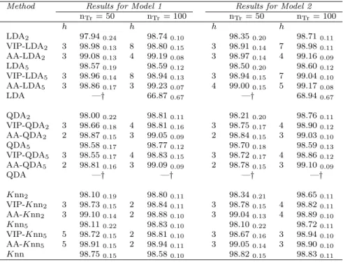
Tables 2.2-2.3 show, for all the methods, the averages of both the accuracy rate, ˆ
a = M( ˆAc) and, in brackets, the number of selected classifiers, ˆcl = M( ˆCl). A measure of variability for ˆa and ˆcl is also provided (i.e. the standard error of the statistic designated by the subscript). In particular, the standard error of ˆa in the
tables below is estimated as: 1 Nreps1/2 ( (1−ˆa)ˆa nT e + n−1 nT eNreps Nreps X l=1 (ˆa−Acˆ l)2 )1/2 .
See [20] for further details.
Model 1 − Sparse class boundaries
x|{y = 0} ∼ 1 2Np(µ0,Σ) + 1 2Np(−µ0,Σ) x|{y = 1} ∼ 1 2Np(µ1,Σ) + 1 2Np(−µ1,Σ) Σ =Ip×p, µ0 = (2,−2,0, . . . ,0)T and µ1 = (2,2,0, . . . ,0)T
Model 2 − Rotated sparse normal
x|{y= 0} ∼Np(Ωpµ0,ΩpΣ0ΩTp)
x|{y= 1} ∼Np(Ωpµ1,ΩpΣ1ΩTp)
Ωp is a p×p rotation matrix sampled once according to the Haar measure, µ0 =
(3,3,3,0, . . . ,0)T, µ
1 = (0, . . . ,0)T.
Σ0 and Σ1 are block diagonal, with blocks Σ (1)
0 (3×3 matrix with diagonal entries
equal to 2 and off-diagonal entries equal to 12), Σ(1)1 = Σ(1)0 −I3×3 and Σ (2)
0 = Σ
(2) 1
((p−3)×(p−3) matrix with diagonal entries equal to 1 and off-diagonal entries equal to 12). - Σ(1)0 3×3 = 2 0.5 0.5 0.5 2 0.5 0.5 0.5 2 - Σ(1)1 3×3 = 1 0.5 0.5 0.5 1 0.5 0.5 0.5 1
- Σ(2)0 (p−3)×(p−3) = Σ(2)1 (p−3)×(p−3) = 1 0.5 . . . 0.5 0.5 1 . . . 0.5 .. . . .. ... 0.5 0.5 . . . 1
Model 3 − Independent features
x|{y= 0} ∼Np(µ, Ip×p)
x|{y= 1} is simulated from a distribution of p independent components each with a standard Laplace distribution, L(0,1).
µ = (1/√p)(1, . . . ,1,0. . . ,0)T is the mean vector of the normal distribution with p/2 non-zero components.
Model 4 − t-distributed features
x|{y=r}=µr+Zr/ p (Ur/νr) r = 0,1 Zr ∼Np(0,Σr) independent of Ur ∼χ2νr. µ0 = (1, . . . ,1,0. . . ,0) T with 10 non-zero components, µ1 = 0, ν0 = 2, ν1 = 1, Σ0 = Σj,k where Σj,j = 1, Σj,k = 0.5 if
max(j, k)≤10 andj 6=k, Σj,k = 0 otherwise, and Σ1 =Ip×p.
RP Methodd Results for Model 1 Results for Model 2
LDA2 50.59 0.49(101.000.00) 93.880.25(101.000.00) ESA-LDA2 50.670.43(70.304.43) 92.730.32(38.574.34) GA-LDA2 50.54 0.43(52.270.80) 93.430.25(45.670.95) LDA5 50.270.38(101.000.00) 94.160.23(101.000.00) ESA-LDA5 49.850.38(58.804.25) 93.300.28(27.733.83) GA-LDA5 49.920.40(51.700.64) 93.860.21(42.970.97)
Table 2.2: Accuracy rates with standard errorsand (number of selected classifiers with
standard errors) for Models 1 and 2.
The overall results showed in Tables 2.2 and 2.3 demonstrate that removing redundant classifiers from the RP ensemble (rather than using the entire set) could determine a performance gain. Moreover, in all the situations where it occurs (Model 1, Model 3 and Model 4 with d= 2), the ESA tends to be more effective than the
RP Methodd Results for Model 3 Results for Model 4 LDA2 50.39 0.86(101.000.00) 64.26 1.64(101.000.00) ESA-LDA2 50.470.82(66.973.98) 64.991.35(46.236.05) GA-LDA2 50.38 0.88(55.370.98) 63.53 1.54(50.730.98) LDA5 52.720.70(101.000.00) 69.681.09(101.000.00) ESA-LDA5 52.390.69(60.874.82) 69.351.00(49.075.51) GA-LDA5 52.220.66(53.070.90) 68.981.07(50.600.99)
Table 2.3: Accuracy rates with standard errors and (number of selected classifiers with
standard errors) for Models 3 and 4.
GA in selecting the smallest subset of base classifiers that provide the best possible accuracy.
2.4.2.2 Real data examples
Seven different high-dimensional datasets available from the UC Irvine (UCI) Ma-chine Learning Repository [76] have been used to evaluate the method performances. In all the real applications, the ESA has been trained for nBest= 5 solutions.
Eye state detection dataset
The electroencephalogram eye state dataset provides information about p = 14 electroencephalogram measurements on 14980 patients. The task is to use these information to determine whether the eye is either open (class 0, size 8256) or closed (class 1, size 6723).
Ionosphere dataset
The ionosphere dataset contains p = 32 high-frequency antenna measurements for 315 observations. Specifically, radar returns from the ionosphere are classified as either suitable for further analysis (class 0, size 225) or not (class 1, size 126) de-pending on the evidence for free electrons.
Down’s syndrome diagnoses in mice
The mice dataset consists of the expression levels of p = 68 proteins/protein mod-ifications on 1080 mice. The task is to classify mice as healthy (class 0, size 570) or affected by Down’s syndrome (class 1, size 507) on the basis of their protein expression measurements.
Hill-valley dataset
The hill-valley dataset consists of 1212 observations, each of them representing 100 points on a two-dimensional graph. When plotted in sequence, the points create either a hill (a“bump” in the terrain; class 0, size 600) or a valley (a “dip” in the terrain; class 1, size 612). The goal of the analysis is to classify the terrain on the basis of a vector of dimension p= 100.
Musk dataset
The musk dataset consists of 6598 molecules classified as musk (class 0, size 1016)
or non-musk (class 1, size 5581), based on p= 166 features that describe the exact
shape or the conformation of each molecule. The goal is to learn to predict whether new molecules will be musks or non-musks.
Cardiac arrhythmia dataset
The cardiac arrhythmia dataset contains observations on 452 patients. The aim is to distinguish between the presence (class 0, size 245) and absence (class 1, size 207) of cardiac arrhythmia using results from p = 190 electrocardiogram (ECG) measurements.
Human activity recognition dataset
The human activity recognition dataset contains p = 561 measurements, recorded from a waist-mounted smartphone with embedded inertial sensors while a subject is performing an activity. The initial dataset has been subsampled in order to include only two of the six original activity: walking and laying. The final dataset consists of 1226 walking” observations (class 0) and 1407 “laying” observations (class 1).
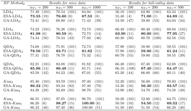
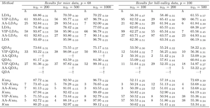
As noticed for the simulation results, for the real data applications too, the classification performances of the ESA are generally in line with those yielded by the other competitors. Moreover, in some real examples (e.g. for the mice and
the hill-valleydatasets), the improvement in classification accuracy provided by our
proposal is particularly evident.
The inspection of the values in brackets (i.e. the number of classifiers selected for the final ensemble), clearly shows the tendency of the ESA (already mentioned in Section 2.4.2.1for the simulated examples) to consider small subsets of classifiers.
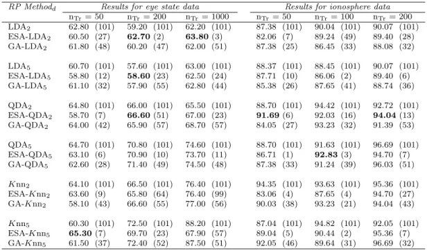
RP Methodd Results for eye state data Results for ionosphere data nTr= 50 nTr= 200 nTr = 1000 nTr= 50 nTr= 100 nTr= 200 LDA2 62.80 (101) 59.20 (101) 62.20 (101) 87.38 (101) 90.04 (101) 90.07 (101) ESA-LDA2 60.50 (27) 62.70(2) 63.80(3) 82.06 (7) 89.24 (49) 89.40 (28) GA-LDA2 61.80 (48) 60.20 (47) 62.00 (51) 87.38 (25) 86.45 (33) 88.08 (32) LDA5 60.70 (101) 57.60 (101) 63.00 (101) 88.37 (101) 88.45 (101) 90.07 (101) ESA-LDA5 58.80 (12) 58.60(23) 62.50 (24) 87.71 (10) 86.06 (2) 89.40 (6) GA-LDA5 61.10 (32) 57.90 (55) 62.80 (44) 85.38 (26) 87.65 (41) 88.74 (36) QDA2 64.80 (101) 66.00 (101) 65.50 (101) 88.70 (101) 94.42 (101) 92.72 (101) ESA-QDA2 58.70 (7) 66.60(51) 67.00 (23) 91.69(6) 92.03 (16) 94.04(13) GA-QDA2 64.00 (42) 65.90 (57) 68.70 (57) 84.05 (27) 93.23 (32) 91.39 (53) QDA5 64.70 (101) 70.80 (101) 74.60 (101) 88.70 (101) 91.63 (101) 96.69 (101) ESA-QDA5 63.10 (6) 70.90 (10) 73.70 (11) 86.71 (1) 92.83(3) 94.70 (7) GA-QDA5 62.60 (28) 71.40 (49) 74.50 (48) 87.38 (33) 91.24 (39) 96.03 (51) Knn2 64.10 (101) 66.50 (101) 76.40 (101) 94.35 (101) 93.63 (101) 95.36 (101) ESA-Knn2 63.60 (9) 65.80 (64) 76.40 (99) 83.06 (4) 87.65 (4) 94.70 (27) GA-Knn2 58.10 (43) 66.60 (55) 77.00 (56) 90.03 (38) 93.23 (21) 94.04 (43) Knn5 60.30 (101) 72.50 (101) 88.20 (101) 87.04 (101) 94.82 (101) 92.05 (101) ESA-Knn5 65.30(7) 69.70 (23) 67.90 (57) 89.04 (5) 90.44 (2) 95.36 (7) GA-Knn5 61.50 (37) 72.40 (52) 87.50 (51) 92.05 (46) 89.64 (31) 96.69 (32)
Table 2.4: Accuracy rates and (number of selected classifiers) for the eye state and ionosphere data.
In addition to the discussed outcomes, a further analysis was implemented with the aim to compare the performances of the considered post-pruning approaches (ESA and GA) with those yielded by the new extensions suggested by Cannings and Samworth to increase the RP ensemble diversity. In particular, Table 2.8 contains the accuracy rates for the mice and the hill-valley datasets obtained by employing the leave-one-out (loo) estimator for all the three base classifiers (i.e. LDA, QDA, Knn) in the RP ensemble and by performing the new procedures introduced in the discussion on [20]. Specifically, with “Random” we denote the authors’ proposal of randomly choosing, on each projection, the base classifier; with “All”, instead, we refer to the alternative of trying all the base methods on each projection and, than, selecting the most performing one.
Results from this numerical study reveals once again that diversity is a key issue in classifier combination. Moreover, our proposal of aposteriori selecting the most diverse and accurate set of the ensemble classifiers according to the MB parameters, seems to provide good results. In fact, the accuracy rates yielded by the ESA are always better than (or comparable with) those achieved by inducing diversity during the RP ensemble generating process.
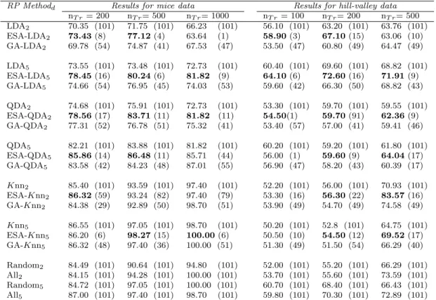
RP Methodd Results for mice data Results for hill-valley data nT r= 200 nT r= 500 nT r= 1000 nT r= 100 nT r= 200 nT r= 500 LDA2 71.49 (101) 70.54 (101) 64.94 (101) 56.10 (101) 62.90 (101) 63.34 (101) ESA-LDA2 73.55(19) 76.60(8) 67.53 (8) 55.40 (4) 71.00(1) 64.89(4) GA-LDA2 72.41 (61) 68.80 (41) 71.43 (39) 53.50 (47) 59.80 (53) 64.04 (34) LDA5 74.23 (101) 76.26 (101) 72.73 (101) 60.40 (101) 80.40 (101) 69.94 (101) ESA-LDA5 81.98(6) 80.59(8) 72.73 (14) 63.90(11) 80.90(68) 77.95(27) GA-LDA5 74.34 (50) 78.34 (43) 77.92 (46) 60.30 (50) 80.70 (100) 82.58 (53) QDA2 74.68 (101) 75.91 (101) 72.73 (101) 57.90 (101) 58.90 (101) 59.55 (101) ESA-QDA2 78.56(17) 83.71(11) 81.82 (11) 57.90 (101) 59.90(16) 61.24(11) GA-QDA2 77.31 (52) 76.78 (51) 75.32 (41) 60.70 (55) 59.80 (52) 59.55 (39) QDA5 82.21 (101) 83.88 (101) 81.82 (101) 66.40 (101) 67.40 (101) 62.08 (101) ESA-QDA5 85.86(14) 86.48(11) 85.71 (44) 66.10 (100) 67.40(101) 64.47(8) GA-QDA5 83.58 (42) 84.23 (48) 87.01 (55) 65.20 (44) 66.80 (60) 60.11 (40) Knn2 85.40 (101) 93.59 (101) 97.40 (101) 52.20 (101) 56.00 (101) 70.93 (101) ESA-Knn2 86.32(59) 93.24 (82) 97.40 (79) 53.30 (16) 56.30(22) 83.57(16) GA-Knn2 84.38 (29) 92.89 (50) 98.70 (51) 53.90 (49) 54.70 (49) 74.58 (49) Knn5 86.55 (101) 97.05 (101) 98.70 (101) 50.20 (101) 52.80 (101) 64.75 (101) ESA-Knn5 86.20 (6) 98.27(15) 100.00(6) 50.50 (10) 54.50(12) 69.52(17) GA-Knn5 86.32 (48) 97.40 (36) 100.00 (51) 51.30 (49) 51.50 (54) 66.29 (40)
Table 2.5: Accuracy rates and (number of selected classifiers) for the mice and hill-valley data.
2.5
Variable Importance in ensembles
As discussed in the previous section, ensemble of classifiers proved to be a very useful tool for excellently solving many classification problems. In particular, by combining the predictions of several (potentially weak) base classifiers, ensembles allow to better improve both the generalizability and the robustness of the final estimates. Hovewer, these notable performances carry a remarkable drawback that strongly affects ensemble algorithms. Namely, methods in this class could be con-sidered as “black-boxes” which take in input and give out just predictions, without worrying too much about the underlying mechanism. In this sense, one of the main shortcomings of ensembles is the fact that, differently from the single classifier, they loose connection with the original variables and, therefore, do not provide any in-sight about the feature importance in the classification process.
Among the proposed ensembles of classifiers, the Random Forest procedure rep-resents one of the most commonly used. The RF algorithm was firstly introduced by Breiman in 2001 [16] as an ensemble learning technique which combines the pre-dictions ofB1weak learners (classification or regression trees) in order to boost their
individual performances. In order to help the interpretation of the final outcome and to overcome the ensemble limits above-discussed, the possibility of efficiently
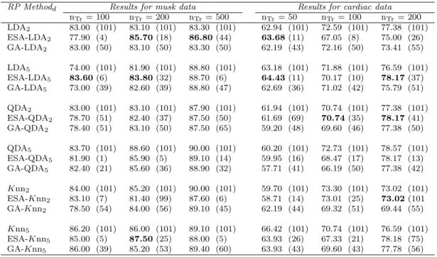
RP Methodd Results for musk data Results for cardiac data nTr= 100 nTr= 200 nTr = 500 nTr= 50 nTr= 100 nTr= 200 LDA2 83.00 (101) 83.10 (101) 83.30 (101) 62.94 (101) 72.59 (101) 77.38 (101) ESA-LDA2 77.90 (4) 85.70(18) 86.80(44) 63.68(11) 67.05 (8) 75.00 (26) GA-LDA2 83.00 (50) 83.10 (50) 83.30 (50) 62.19 (43) 72.16 (50) 73.41 (55) LDA5 74.00 (101) 81.90 (101) 88.80 (101) 63.18 (101) 71.88 (101) 76.59 (101) ESA-LDA5 83.60(6) 83.80(32) 88.70 (6) 64.43(11) 70.17 (10) 78.17(37) GA-LDA5 73.00 (39) 82.60 (39) 88.80 (47) 62.69 (36) 71.02 (42) 75.79 (51) QDA2 83.00 (101) 83.10 (101) 87.90 (101) 61.94 (101) 70.74 (101) 77.38 (101) ESA-QDA2 78.70 (51) 82.40 (37) 87.50 (50) 61.69 (69) 70.74(35) 78.17(41) GA-QDA2 78.40 (51) 83.10 (50) 87.50 (65) 59.20 (48) 69.60 (46) 77.38 (50) QDA5 83.70 (101) 88.60 (101) 90.00 (101) 60.20 (101) 72.73 (101) 78.57 (101) ESA-QDA5 81.90 (1) 85.90 (5) 89.10 (14) 59.95 (16) 68.47 (17) 78.17 (13) GA-QDA5 82.40 (21) 85.60 (36) 88.90 (32) 57.71 (41) 66.19 (50) 77.38 (42) Knn2 84.00 (101) 85.20 (101) 90.00 (101) 59.70 (101) 73.30 (101) 73.02 (101) ESA-Knn2 83.10 (7) 81.40 (99) 87.60 (6) 58.71 (14) 73.01 (25) 73.02(101 GA-Knn2 78.50 (54) 84.00 (56) 89.10 (45) 62.19 (44) 69.32 (51) 69.44 (55) Knn5 86.20 (101) 86.00 (101) 89.10 (101) 66.42 (101) 70.74 (101) 76.59 (101) ESA-Knn5 85.00 (5) 87.50(25) 88.00 (5) 63.93 (26) 67.33 (21) 78.18 (75) GA-Knn5 86.00 (39) 85.20 (53) 89.40 (60) 63.93 (43) 69.60 (43) 77.78 (56)
Table 2.6: Accuracy rates and (number of selected classifiers) for the musk and cardiac arrhythmia data.
ranking the input features according to their importance was considered since the first formulation of the algorithm. In particular, in RFs, the strength of a generic u-th feature can be measured by averaging, over all the trees in the forest, the dif-ference between the initial Out-Of-Bag (OOB) error and the OOB error computed after permuting the values for theu-th variable in the OOB sample. The final score is than obtained by normalizing these differences with their standard deviations. Inspired both by the RF process for variable ranking and the work of Montanari and Lizzani [85] on projection pursuits, the main idea in this work is to use the information provided by the RP ensemble classifier so as to mitigate the typical lack of interpretability which characterizes of ensembles.
2.5.1
Variable ranking for the RP ensemble
A still open issue in [20] is “to understand the properties of the variable ranking
induced by the RP ensemble classifier”. In fact, despite such classifier highly
im-proves the classification accuracy, it does not allow to identify the variables with the highest discriminative power, as a single classifier does.
In the discussion on the paper by Cannings and Samworth [20], several contributors mention the potential use of sparse RPs (e.g. Axis-Aligned Random Projections,
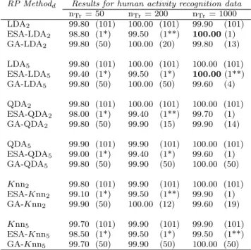
RP Methodd Results for human activity recognition data nTr= 50 nTr= 200 nTr= 1000 LDA2 99.80 (101) 100.00 (101) 99.90 (101) ESA-LDA2 98.80 (1*) 99.50 (1**) 100.00(1) GA-LDA2 99.80 (50) 100.00 (20) 99.80 (13) LDA5 99.80 (101) 100.00 (101) 100.00 (101) ESA-LDA5 99.40 (1*) 99.50 (1*) 100.00(1**) GA-LDA5 99.80 (50) 100.00 (50) 99.60 (4) QDA2 99.80 (101) 100.00 (101) 100.00 (101) ESA-QDA2 98.00 (1*) 99.40 (1**) 99.70 (1) GA-QDA2 99.80 (50) 99.90 (15) 99.90 (14) QDA5 99.90 (101) 99.90 (101) 100.00 (101) ESA-QDA5 99.00 (1*) 99.40 (1*) 99.60 (1) GA-QDA5 99.80 (50) 99.90 (50) 100.00 (50) Knn2 99.80 (101) 99.90 (101) 100.00 (101) ESA-Knn2 99.10 (1*) 99.50 (1**) 99.90 (1) GA-Knn2 99.90 (50) 100.00 (12) 99.60 (19) Knn5 99.70 (101) 99.90 (101) 99.90 (101) ESA-Knn5 98.50 (1*) 99.50 (1*) 99.50 (1**) GA-Knn5 99.70 (50) 99.90 (50) 100.00 (50)
*means that all the π
i are equal and, thus, the ESA does not start.
**means that theH matrix does not contain n Best = 5 different values and, thus, only smaller solutions of
nBest (corresponding to the number of distinct hi,v,
i6=v) are explored.
Table 2.7: Accuracy rates and (number of selected classifiers) for the human activity recognition data.
AA-RP) to measure the importance of each input variable. Gataric, for example, numerically demonstrates that performing a majority vote scheme across the B1
projections ˆ a∗u = 1 B1 B1 X i=1 1{(AT iAi)u,u=1} u= 1,· · · , p (2.3)
could provide a good estimation of the classification power for each feature u. In this work, in the same spirit, a specific coefficient, called Variable Importance
in Projection (VIP), is introduced so as to evaluate the importance of each input
variable.
Following Montanari and Lizzani (2001), for the u-th variable theImportance
Coef-ficient (CI) is defined as
CIui = d X q=1 |auqi|su q Pp z=1(auzisu) 2 i= 1,· · · , B1
RP Methodd Results for mice data Results for hill-valley data nT r = 200 nT r= 500 nT r= 1000 nT r = 100 nT r= 200 nT r= 500 LDA2 70.35 (101) 71.75 (101) 66.23 (101) 56.10 (101) 63.20 (101) 63.76 (101) ESA-LDA2 73.43(8) 77.12(4) 63.64 (1) 58.90(3) 67.10(15) 63.06 (10) GA-LDA2 69.78 (54) 74.87 (41) 67.53 (47) 53.50 (47) 60.80 (49) 64.47 (49) LDA5 73.55 (101) 73.48 (101) 72.73 (101) 60.40 (101) 69.60 (101) 68.82 (101) ESA-LDA5 78.45(16) 80.24(6) 81.82 (9) 64.10(6) 72.60(16) 71.91(9) GA-LDA5 74.66 (54) 76.95 (45) 74.03 (53) 59.60 (42) 66.30 (50) 68.82 (43) QDA2 74.68 (101) 75.91 (101) 72.73 (101) 53.30 (101) 59.70 (101) 59.55 (101) ESA-QDA2 78.56(17) 83.71(11) 81.82 (11) 54.50(1) 59.70(91) 62.36(9) GA-QDA2 77.31 (52) 76.78 (51) 75.32 (41) 53.40 (57) 57.00 (41) 59.41 (46) QDA5 82.21 (101) 83.88 (101) 81.82 (101) 60.20 (101) 59.20 (101) 61.80 (101) ESA-QDA5 85.86(14) 86.48(11) 85.71 (44) 56.00 (1) 59.60(9) 64.04(17) GA-QDA5 83.58 (42) 84.23 (48) 87.01 (55) 56.90 (47) 58.20 (43) 60.39 (17) Knn2 85.40 (101) 93.59 (101) 97.40 (101) 52.20 (101) 56.00 (101) 70.93 (101) ESA-Knn2 86.32(59) 93.24 (82) 97.40 (79) 53.30 (16) 56.30(22) 83.57(16) GA-Knn2 84.38 (29) 92.89 (50) 98.70 (51) 53.90 (49) 54.70 (49) 74.58 (49) Knn5 86.55 (101) 97.05 (101) 98.70 (101) 50.20 (101) 52.8 (101) 64.75 (101) ESA-Knn5 86.20 (6) 98.27(15) 100.00(6) 50.50 (10) 54.50(12) 69.52(17) GA-Knn5 86.32 (48) 97.40 (36) 100.00 (51) 51.30 (49) 51.50 (54) 66.29 (40) Random2 84.49 (101) 90.64 (101) 94.80 (101) 52.00 (101) 55.20 (101) 66.29 (101) All2 84.15 (101) 94.28 (101) 100.00 (101) 53.70 (101) 55.60 (101) 73.59 (101) Random5 84.72 (101) 97.05 (101) 100.00 (101) 60.70 (101) 68.40 (101) 66.43 (101) All5 87.00 (101) 97.40 (101) 98.70 (101) 59.80 (101) 70.30 (101) 72.89 (101)
Table 2.8: Accuracy rates and (number of selected classifiers) for the mice and hill-valley data obtained by using the loo estimator.
whereauqi indicates the attributeucoefficient in theq-th vector of thed-dimensional
random projection solution and su the variability (i.e. the standard deviation) of
each attribute.
The Variable Importance in Projection for feature u is then obtained as V IPu = median
i=1,...,B1
CIui. (2.4)
The median is used here so as to mitigate the effects on the V IP of potential not-so-good projections. By computing the VIP it is possible to rank the input features and highlight the most relevant ones for classification purposes.
The number of variables to be kept is decided by the user; a possible strategy is to explore all the solutions and, then, retain only the first h variables that minimize the test error estimate.
2.5.2
Empirical analysis
Performances of the VIP criterion have been evaluated in both simulated and real data applications.
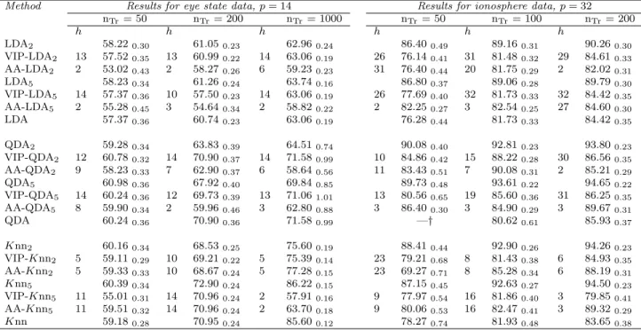
As a first step, for each simulated scenario, the capability of the measure in 2.4 to recognize the actual important variables was tested and, then, compared to the one described in 2.3. Secondly, both the VIP (RP-VIP) and the proposal by Gataric (AA-RP) were applied within the RP ensemble classifier framework with the specific aim to address classification issues. In this case, the input variables of each dataset have been initially ranked according to the two discussed criteria, each computed on B1 = 101 d-dimensional Gaussian-distributed RP matrices selected within blocks
of B2 = 50 possible solutions; then, three base classifiers (LDA, QDA, Knn) were
performed on 100 different training sets, by using, for each method, only the first h variables yielding the largest estimate of the training accuracy.
In addition to the accuracy rates provided by the RP-VIP and the AA-RP ensemble classifiers, results from the RP ensemble classifier in [20] and the “standard” classi-fication (i.e. by applying the base