Modeling, forecasting and trading the EUR exchange rates with hybrid rolling genetic algorithms: support vector regression forecast combinations

Sermpinis, G., Stasinakis, C., Theofilatos, K. and Karathanasopoulos,

A. (2015) Modeling, forecasting and trading the EUR exchange rates with

hybrid rolling genetic algorithms: support vector regression forecast

combinations.

European Journal of Operational Research

, 247(3), pp.

831-846. (doi:

10.1016/j.ejor.2015.06.052

)

This is the author’s final accepted version.

There may be differences between this version and the published version.

You are advised to consult the publisher’s version if you wish to cite from

it.

http://eprints.gla.ac.uk/108101/

Deposited on: 21 July 2015

Enlighten – Research publications by members of the University of Glasgow http://eprints.gla.ac.uk33640

Modeling, Forecasting and Trading the EUR Exchange Rates with Hybrid

Rolling Genetic Algorithms – Support Vector Regression Forecast Combinations

Georgios Sermpinis* Charalampos Stasinakis** Konstantinos Theofilatos*** Andreas Karathanasopoulos**** June 2015 Abstract

The motivation of this paper is to introduce a hybrid Rolling Genetic Algorithm – Support Vector Regression (RG-SVR) model for optimal parameter selection and feature subset combination. The algorithm is applied to the task of forecasting and trading the EUR/USD, EUR/GBP and EUR/JPY exchange rates. The proposed methodology genetically searches over a feature space (pool of individual forecasts) and then combines the optimal feature subsets (SVR forecast combinations) for each exchange rate. This is achieved by applying a fitness function specialized for financial purposes and adopting a sliding window approach. The individual forecasts are derived from several linear and non-linear models. RG-SVR is benchmarked against genetically and non-genetically optimized SVRs and SVMs models that are dominating the relevant literature, along with the robust ARBF-PSO neural network. The statistical and trading performance of all models is investigated during the period of 1999-2012. As it turns out, RG-SVR presents the best performance in terms of statistical accuracy and trading efficiency for all the exchange rates under study. This superiority confirms the success of the implemented fitness function and training procedure, while it validates the benefits of the proposed algorithm.

Keywords

Genetic Algorithms, Support Vector Regression, Feature Subset, Forecast Combinations, Exchange Rates

*University of Glasgow Business School, University of Glasgow, Adam Smith Building, Glasgow, G12 8QQ, UK ([email protected])

**University of Glasgow Business School, University of Glasgow, Adam Smith Building, Glasgow, G12 8QQ, UK ([email protected])

***

Pattern Recognition Laboratory, Dept. of Computer Engineering & Informatics, University of Patras, 26500, Patras, Greece ([email protected])

**** Andreas Karathanasopoulos Royal Docklands Business School, University of East London, ([email protected])

1. INTRODUCTION

Forecasting financial time series appears to be a challenging task for the scientific community because of its non-linear and non-stationary structural nature. On one hand, traditional statistical methods fail to capture this complexity, while on the other hand non-linear techniques present promising empirical evidence. However, their practical limitations and the expertise required to optimize their parameters are creating skepticism on their utility.

This study introduces a hybrid Rolling Genetic Algorithm – Support Vector Regression (RG-SVR) algorithm for optimal parameter selection and feature subset combination when applied to the task of forecasting and trading the EUR/USD, EUR/GBP and EUR/JPY exchange rates. The proposed model genetically searches over a feature space (pool of individual forecasts) and then combines the optimal feature subsets for each exchange rate. A novel fitness function specialized for financial purposes is used to simultaneously minimize the error of the obtained forecasts, increase the profitability of the final forecast combination and reduce the complexity of the algorithm. This is crucial in financial applications, where statistical accuracy is not always synonymous with the financial profitability of the deriving forecasts. The reduced complexity of the algorithm decreases the computational cost of the proposed methodology and makes it ideal for trading applications, where time efficiency is important. At the same time, it acts as a protection against overfitting and impeded generalization abilities. The model employs a sliding window training approach and is capable of capturing the time-varying relationship that dominates the financial trading series.

RG-SVR is benchmarked against seven models. Their statistical and trading performance is compared during the period of 1999-2012. The rationale behind the selection of the benchmarks is twofold. Firstly, Support Vector Machine (SVM) and Support Vector Regression (SVR) architectures with genetically and non-genetically optimized parameters are dominant in the relevant literature. The six most popular and promising variants are identified and included in the study (see section 4.3). Secondly, it would be unfair to compare the hybrid RG-SVR only with hybrids of the same methodology class, especially when other proposed methodologies have shown statistical and trading superiority in a similar task. One such example is the hybrid Neural Network (NN) that combines Adaptive Radial Basis Functions with Particle Swarm Optimization (ARBF-PSO), as introduced recently by Sermpinis et al. (2013). The authors apply ARBF-PSO to the task of forecasting and trading the same exchange rates that the present study is investigating. Their results show that ARBF-PSO is outperforming several linear and non-linear models, while its structural complexity is not high. Consequently, ARBF-PSO’s selection as a benchmark to this application is required and justified.

To the best of our knowledge, the proposed RG-SVR methodology has not been presented in the literature. Similar hybrid applications exist but they are either limited in classification problems (Min

et al. (2006), Huang and Wang (2006), Wu et al. (2007), Dunis et. al. (2013)) or the Genetic Algorithm (GA) does not extend to optimal feature subset selection (Pai et al. (2006), Chen and Wang (2007), Yuan (2012)). In addition to this fact, the RG-SVR hybrid is the first GA hybrid SVR algorithm that deploys v-SVR models, minimizes the number of support vectors and applies a specialized loss function and a sliding window training approach. A detail comparison of the algorithm and the previous two algorithms is presented in the next section. The genetically optimized SVM model (GA-SVM) proposed by Min et al. (2006), Huang and Wang (2006), Wu et al. (2007) and Dunis et. al. (2013) and the genetically optimized ε-SVR model (GA-εSVR) proposed by Pai et al. (2006), Chen and Wang (2007) and Yuan (2012) will act as benchmarks to the RG-SVR algorithm. Compared to non-adaptive algorithms presented in the literature, the proposed model does not require from the practitioner to follow any time-consuming optimization approach (such as cross validation or grid search) and is free from the data snooping bias (all parameters of RG-SVR are optimized in a single optimization procedure).

From the results of this analysis, it emerges that RG-SVR presents the best performance in terms of statistical accuracy and trading efficiency for all exchange rates under study. RG-SVR’s trading performance and forecasting superiority not only confirms the success of the implemented fitness function, but also validates that applying GAs in this hybrid model to optimize the SVR parameters is more efficient compared to the optimization approaches (cross validation and grid search algorithms), that dominate the relevant literature.

The rest of the paper is organized as follows. Section 2 is a literature review of previous relevant research on SVMs and SVRs in forecasting. A detailed description of the study’s dataset, the EUR/USD, EUR/GBP and EUR/JPY European Central Bank (ECB) fixing series, is presented in Section 3. Section 4 includes the complete description of the hybrid RG-SVR model, while the statistical and trading performance of the implemented models is presented in sections 5 and 6 respectively. The concluding remarks are provided in section 7. The essential theoretical background for the complete understanding of the proposed methodology is given in the appendix section, along with the technical characteristics of the models used in this study.

2. LITERATURE REVIEW

SVMs were originally developed for solving classification problems in pattern recognition frameworks. The introduction of Vapnik’s (1995) insensitive loss function has extended their use in non-linear regression estimation problems. SVRs’ main advantage is that they provide global and unique solutions and do not suffer from multiple local minima, while they present a remarkable

ability of balancing model accuracy and model complexity (Kwon and Moon (2007) and Suykens (2005)).

The literature of SVM and SVR applications is voluminous, especially when they are applied in financial tasks. This study aims to delve deeper into their hybrid structures that are already very popular (Lo, 2000). Lee et al. (2004) propose the multi-category SVM as an extension of the traditional binary SVM and apply it in two different case studies with promising results. They note that their proposed methodology can be a useful addition to the class of nonparametric multi-category classification methods. Liu and Shen (2006) advance the previous mentioned approach by presenting the multi-category ψ-learning methodology. The main advantage of their method is that the convex SVM loss function is replaced by a non-convex ψ-loss function, which leads to smaller number of support vectors and sparser solution. Martens et al. (2007) introduce two extraction techniques for SVMs and prove their utility in a series of tests. Hsu et al.(2009) integrate SVR in a two-stage architecture for stock price prediction and present empirical evidence that show that its forecasting performance can be significantly enhanced compared to a single SVR model. Lu et al. (2009) and

Yeh et al. (2011) propose also hybrid SVR methodologies for forecasting the TAIEX index and

conclude that that they perform better than simple SVR approaches and other autoregressive models. Wu and Liu (2007) introduce the Robust Truncated Hinge Loss SVM and claim that their method can overcome drawbacks of traditional SVM models, such as the outliers’ sensitivity in the training sample and the large number of support vectors. Huang et al. (2010) forecast the EUR/USD, GBP/USD, NZD/USD, AUD/USD, JPY/USD and RUB/USD exchange rates with a hybrid chaos-based SVR algorithm. In their application, they confirm the forecasting superiority of their proposed technique compared to chaos-based NNs and several traditional non-linear models. Lin and Pai (2010) introduce a fuzzy SVR model for forecasting indices of business cycles, Kim and Sohn (2010) forecast the credit score of small and medium enterprises with SVM, while Wu and Akbarov (2011) apply successfully weighted SVRs to the task of forecasting warranty claims. Moreover, Jiang and He (2012) propose a hybrid SVR that incorporates the Grey relational grade weighting function. When applied to financial time series forecasting, the local Grey SVR outperforms locally weighted counterparts in terms of computational speed and prediction accuracy. A hybrid architecture for computer products’ sales forecasting is also introduced by Lu (2014) based on SVR and multivariate adaptive regression splines.

Most recently, Yao et al. (2015) use SVRs in the credit risk modeling framework. Specifically, the authors evaluate the predictive ability of SVR over recovery rates of defaulted corporate instruments between 1985 and 2012. The results show the superiority of the SVR techniques in forecasting these rates compared to other commonly used methods, such as linear regression, fractional response regression and the two-stage methodology. Finally, Geng et al. (2015) present a forecast competition of methodologies, such as NNs, SVM, decision trees and majority voting classifiers, to the task of

predicting financial distress of listed Chinese companies. The empirical evidence of that study shows that NNs outperform the SVM, but they acknowledge that this is contradicting previous literature. Similar applications to the proposed hybrid approach of this study can be found in the literature. For example Min et al. (2006) and Wu et al. (2007) use hybrid GA-SVM models in order to forecast the bankruptcy risk. In both applications, the GAs optimizes the parameters of the SVM and selects the financial ratios that most affect bankruptcy. Dunis et al. (2013) developed a GA-SVM algorithm and applied it to the task of trading the daily and weekly returns of the FTSE 100 and ASE 20 indices. This approach deals with financial forecasting as a classification problem and has limited applicability. In financial forecasting, though, it is crucial to obtain forecasts that predict not only the sign but also the size of the examined financial indices.

Pai et al. (2006) apply epsilon SVR with genetically optimized parameters (GA-εSVR) in forecasting

exchange rates, while Chen and Wang (2007) forecast the tourist demand in China with a similar model. Yuan (2012) suggests that a GA-εSVR model is more efficient than traditional SVR and NN models, when applied to the task of forecasting sales volume. All these GA-εSVR applications do not deploy the GA to locate the optimal feature subset but restrict it in optimizing the parameters of the ε -SVR models and select the model’s inputs empirically.

As described in the previous paragraph, a variety of hybrid methodologies combining SVM/SVR models with GAs have been proposed during the last decade. However, the proposed RG-SVR theoretically outperforms them as it deploys v-SVR models, which are more suitable to this problem than SVMs and ε-SVR. SVMs are constrained to classification problems and their applicability is limited. The ε-SVR models require the desired accuracy of the approximation to be specified beforehand and are extremely sensitive to the selection of the ε parameter compared to the sensitivity

of v-SVRs to the v parameter (Schölkopf et al., 2000). Moreover, RG-SVR optimizes on parallel the

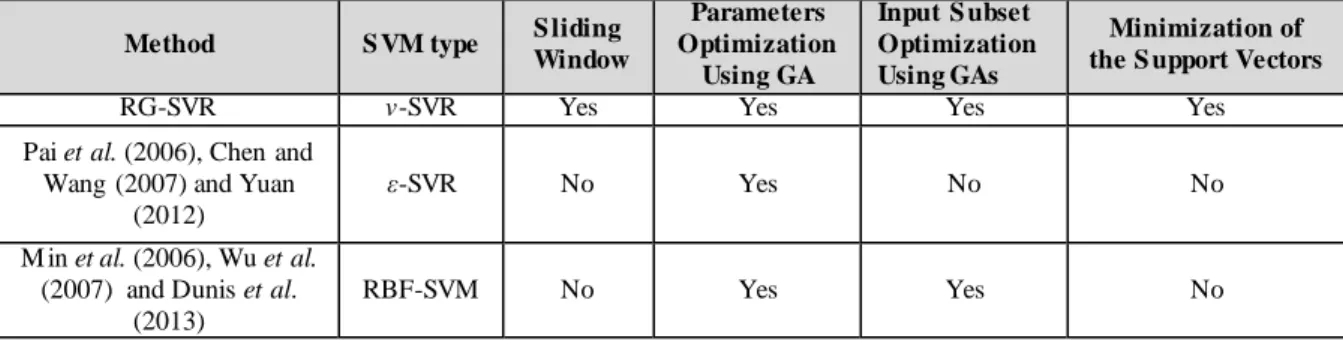
SVR’s parameters and the input’s subset, it deploys a sliding window approach to capture the dynamic nature of the examined financial time series, it employs a specialized loss function and tries to minimize the number of support vectors of the final model in order to improve its generalization abilities. The advantages of RG-SVR over other published methodologies are outlined in table 1.

Table 1: Theoretical Comparison of RG-SVR with other existing hybrid combinations of GAs with SVM/SVR based models

Method S VM type S liding

Window Parameters Optimization Using GA Input S ubset Optimization Using GAs Minimization of the S upport Vectors

RG-SVR v-SVR Yes Yes Yes Yes

Pai et al. (2006), Chen and Wang (2007) and Yuan

(2012) ε-SVR No Yes No No M in et al. (2006), Wu et al. (2007) and Dunis et al. (2013) RBF-SVM No Yes Yes No

3. THE EUR/USD, EUR/GBP AND EUR/JPY EXCHANGE RATES AND RELATED FINANCIAL DATA

The ECB publishes a daily fixing for selected EUR exchange rates. These reference mid-rates are based on a daily concentration procedure between central banks within and outside the European System of Central Banks, which normally takes place at 2.15 p.m. ECT time. The reference exchange rates are published both by electronic market information providers and on the ECB's website shortly after the concentration procedure has been completed.

Although only a reference rate, many financial institutions are ready to trade at the EUR fixing and it is therefore possible to leave orders with a bank for business to be transacted at this level. Thus, the ECB daily fixings of the EUR exchange rate are tradable levels and using them is a more realistic alternative to, say, London closing prices. This superiority for financial institutions to transact at the EUR fixing is a well-known fact by FX markets participants. Financial institutions and institutional investors, and therefore through them, High Net Worth individuals (HNW) would definitely be able to transact at the ECB fixing through their investments with hedge funds, private banks, etc. Smaller private investors could also benefit from reasonably attractive cost conditions (see www.interactivebrokers.com), although they would not be able to transact at the ECB fixing as considered in this study.

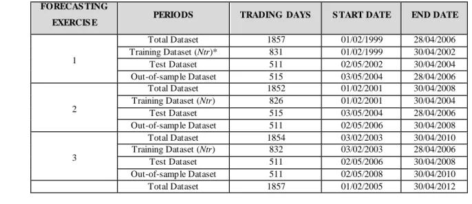
In this paper, the ECB daily fixings of EUR/USD, EUR/GBP and EUR/JPY exchange rates are examined over the period of 01/02/1999 to 30/04/2012. The range of these observations (3395 trading days) is used in four consecutive forecasting exercises. In order to train the RG-SVR, it is necessary to divide the in-sample dataset to training and test subsets (see section 4.1). The test dataset constitutes approximately the 38%1 of the in-sample dataset in each forecasting exercise. The total dataset and the length of each forecasting exercise are presented in the table below.

Table 2: The Total Dataset - Neural Networks’ Training Datasets

* The in-sample dataset is the sum of the training and test dataset

1

This choice is based on in-sample experimentation. We obtain similar trading and statistical in-sample RG-SVR performance for test datasets that constitute the 29% up to the 47% of the in-sample dataset.

FORECAS TING

EXERCIS E PERIODS TRADING DAYS S TART DATE END DATE

1 Total Dataset 1857 01/02/1999 28/04/2006 Training Dataset (Ntr)* 831 01/02/1999 30/04/2002 Test Dataset 511 02/05/2002 30/04/2004 Out-of-sample Dataset 515 03/05/2004 28/04/2006 2 Total Dataset 1852 01/02/2001 30/04/2008 Training Dataset (Ntr) 826 01/02/2001 30/04/2004 Test Dataset 515 03/05/2004 28/04/2006 Out-of-sample Dataset 511 02/05/2006 30/04/2008 3 Total Dataset 1854 03/02/2003 30/04/2010 Training Dataset (Ntr) 832 03/02/2003 28/04/2006 Test Dataset 511 02/05/2006 30/04/2008 Out-of-sample Dataset 511 02/05/2008 30/04/2010 Total Dataset 1857 01/02/2005 30/04/2012

The graph below shows the total dataset for the three exchange rates under study.

Figure 1: The EUR/ USD, EUR/ GBP and EUR/JPY total dataset.

The three observed time series are normal (Jarque-Bera statistics (1980) confirm their non-normality at the 99% confidence interval) containing slight skewness and high kurtosis. They are also non-stationary and hence they are transformed them into three daily series of rate returns2 using the following formula: 1 ln t t t P R P₋   =     [1] Where Rt is the rate of return and Pt is the price level at time t.

The summary statistics of the EUR/USD, EUR/GBP and EUR/JPY return series reveal that the slight skewness and high kurtosis remain. In addition, the Jarque-Bera statistic confirms again their non-normality at the 99% confidence interval.

The aim of these forecasting exercises is to forecast and trade the one day ahead EUR/USD, EUR/GBP and EUR/JPY exchange rate return (E(Rt)). As a first step, we estimate the three return

series with several linear and non-linear models. Then, these estimations are used as potential inputs to the RG-SVR algorithm.

2

Confirmation of their stationary property is obtained at the 1% significance level by both the Augmented Dickey Fuller (ADF) and Phillips-Perron (PP) test statistics.

0 20 40 60 80 100 120 140 160 180 0.4 0.6 0.8 1 1.2 1.4 1.6 1.8 01 F eb 1 99 9 30 Ju n 19 99 26 N ov 1 99 9 28 A pr 2 00 0 27 S ep 2 00 0 28 F eb 2 00 1 01 A ug 2 00 1 03 Ja n 20 02 06 Ju n 20 02 04 N ov 2 00 2 07 A pr 2 00 3 08 S ep 2 00 3 09 F eb 2 00 4 09 Ju l 2 00 4 07 D ec 2 00 4 09 M ay 2 00 5 05 O ct 2 00 5 06 M ar 2 00 6 07 A ug 2 00 6 08 Ja n 20 07 11 Ju n 20 07 07 N ov 2 00 7 11 A pr 2 00 8 10 S ep 2 00 8 11 F eb 2 00 9 15 Ju l 2 00 9 11 D ec 2 00 9 17 M ay 2 01 0 13 O ct 2 01 0 11 M ar 2 01 1 11 A ug 2 01 1 10 Ja n 20 12 EU R /J PY E UR/ US D & E UR/ G BP 1st _{February 1999 to 30}th _{April 2012}

EUR/USD EUR/GBP EUR/JPY 4

Training Dataset (Ntr) 830 01/02/2005 30/04/2008 Test Dataset 511 02/05/2008 30/04/2010 Out-of-sample Dataset 516 03/05/2010 30/04/2012

4. HYBRID RG-SVR MODEL

The hybrid Rolling Genetic – Support Vector Regression (RG-SVR) model for optimal parameter selection and feature subset combination is presented in this section. Initially, the generic architecture of the proposed methodology is described. Then the feature space, in which the model will search for the optimal subsets and combinations, is identified along with the models that are going to be used as benchmarks. The SVR models are more suitable than the classical SVMs ones for this daily forecasting task, as they provide an exact prediction instead of a binary output. The exact prediction enables the effective application of confirmation filters to improve its performance and provide a hint about the strength of the trading signal.

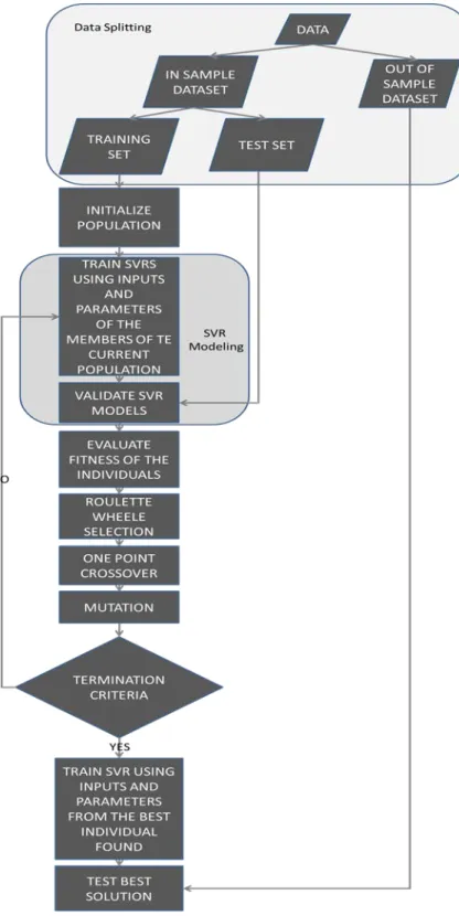
4.1 Architecture

The proposed model genetically searches over the feature space (pool of individual forecasts) and then combines the optimal feature subsets (SVR forecast combinations) for each exchange rate. In order to achieve this, a simple GA is used where each chromosome comprises feature genes that encode the feature subsets and parameter genes that encode the choice of parameters.

The lack of information about the noise’s nature and parameters of the training datasets makes the a

priori ε-margin setting of ε-SVR a difficult task. In order to overcome this and decrease the

computational demands of the methodology, the RBF v-SVR approach is applied in this hybrid RG-SVR model (see appendix A.2). The impact of ε parameter in ε-SVR is much more crucial than the impact of ν in ν-SVR. The ν-SVR method is limiting with an upper and lower bound the number of SVs. In this way, the optimization becomes more stable and the algorithm needs less iterations to find an optimal v value, which would provide accurate results and good generalization properties. The use of the RBF kernel is justified by its extensive use in the literature and its superiority to other types of kernels, when used in financial time series forecasting (Ince and Trafalis (2008) and Lu et al. (2009)). A RBF kernel is in general specified as:

K x x( , )_i =exp(−γ x_i−x 2),γ >0 [2] where γ represents the variance of the kernel function. Consequently, the parameters which should be optimized by the GA are C, v and γ.

Binary representation is used to model the chromosome. Every feature gene is represented with a binary digit. If that gene takes value 1 (0), then this indicates that the relevant feature should be used (not be used) as input. For the parameter genes 50 bits are used, which are specified as follows:

• 10 bits to represent the decimal part of parameter C of SVRs (~ 0.001 precision)

• 10 bits to represent the integer part of the γ parameter of RBF functions ( range [0-1024])

• 10 bits to represent the decimal part of the γ parameter of RBF functions (~ 0.001 precision)

• 10 bits to represent the ν parameter of v-SVR ( range [0-1] with ~ 0.001 precision)

During the initialization step all genes are randomly set with values 0 or 1 with equal probabilities for both of them.

The GA uses the one-point crossover and the mutation operators. The one-point crossover creates two offspring from every two parents. The parents and a crossover point cx are selected at random. The two offsprings are made by both concatenating the genes that precede cx in the first parent with those that follow (and include) cx in the second parent. The probability for selecting an individual as a parent for the crossover operator is called crossover probability and in this application is set to 0.90. Having a high crossover probability enables the model to keep some population for the next generation, hoping to create better new chromosomes from good parts of the old chromosomes. The offspring produced by the crossover operator replaces their parents in the population. The one-point crossover is used for simplicity and to allow bigger blogs of genes to be exchanged during the crossovers. The uniform crossover is usually better only when small mutation probabilities (for example 0.001) are used in order to keep the diversity of chromosomes in the population. In this study, the applied mutation probability is quite big (0.1) and thus the one-point crossover is adequate. The crossover probability is not set to 1 to leave a space for very good solutions of a population to pass through the next generation’s population without being altered. The other variation operator which is deployed is the mutation one. The mutation operator places random values in randomly selected genes with a certain probability named as mutation probability. This operator is very important for avoiding local optima and exploring a larger surface of the search space. This probability is set to 0.1 in order to prevent the algorithm from performing a random search.

For the selection step of the GA, the roulette wheel selection process is used (Holland, 1975). In roulette wheel selection chromosomes are selected according to their fitness. The better the chromosomes are, the more chances to be selected they have. In the proposed approach, elitism is used to raise the evolutionary pressure in better solutions and to accelerate the evolution. In that way, it is assured that the best solution is copied without changes to the new population, so the best solution found can survive at the end of every generation.

More specifically, the selection step is used to resemble the survivor of the fittest principle. In that way better solutions have higher probabilities to provide offspring in the next generation. After the application of selection probability, an intermediate population of solutions is formed with each one of them being identical to the solutions from the previous population. Then, crossover and mutation probabilities are applied to provide offsprings combining solutions from this intermediate population.

Before the application of the crossover operator, the solutions from this intermediate population are used to make pairs of solutions. Some of these pairs are combined using the crossover operator (with the crossover probability) to produce new solutions, while the others are passed to the next intermediate population without being altered. The offspring is derived from the crossover operator and the pairs of solutions that are not recombined form the next intermediate population. After this process, the intermediate population is altered using the mutation operator. In the case of this study, binary mutation is used. If a gene is selected for mutation, then a new random binary value (0 or 1) is constructed and replaces the previous value in this gene. In order to re-assure that no good solutions are missed, elitism is applied. In that way, the best solution is allowed to pass to the next population. The crossover probability is not set to 1 to leave space also for some solutions that are close to optimal not to be recombined, but just change only with the mutation operator (which is applied only in a few genes of the whole chromosome).

For example, assuming population size is N and elitism of one member, the use of the selection operator leads to an intermediate population of N solutions, which form N/2 pairs. Some of these pairs are selected for crossover using the crossover probability and others are passing on for mutation, as they are. When the mutation process is completed, a complete set of final N solutions is derived. The next iteration starts once one solution is randomly replaced with the best solution of the previous generation.

The RG-SVR hybrid performs a rolling window forecasting exercise. The window size is always ten days (two trading weeks). Else the parameters and the inputs of the algorithm are re-estimated every two weeks. This fact allows the model to capture any structural brake in the dataset. Trading series are exhibiting a highly non-linear nature and are affected by a wide range of factors. Mathematical models with fixed parameters are impossible to model them perfectly. Fund managers and professionals apply a range of different models and re-estimate their parameters frequently. The nature of the financial markets and their erratic behavior make impossible a perfect ex-ante configuration of the re-estimation period. Frequent re-estimations dramatically increase the computational time and might induce noise in the estimations3. Infrequent re-estimations will lead to a low trading performance. The ten trading days sliding window approach is selected based on a trade-off between the in-sample trading performances of RG-SVR and the computational time needed for its estimation with the used dataset.

The population of chromosomes is initialized in the training sub-period. The optimal selection of chromosomes is achieved, when their forecasts maximized the proposed loss function (see equation [3] below) in the test-sub period. Then, the optimized parameters and selected predictors of the best

3

Financial markets are vulnerable to behavioural (Froot et. al., 1992) and exogenous factors such as political decisions (Fisman, 2001). These factors are impossible to capture with mathematical models and include noise to time series estimations.

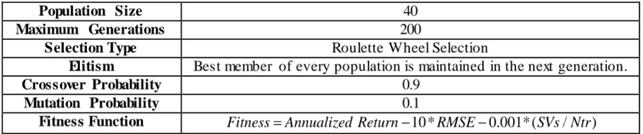
solution are used to train the SVR and produce the final optimized forecast for the next observation. This procedure is repeated in each of the four forecasting exercises. For each of these forecasting exercise, the algorithm stores its optimized C, γ and v parameters and set of optimal predictors. In order to achieve the optimal selection of the feature subsets (individual forecasts) a three-objective fitness function is applied to the hybrid approach. Firstly the annualized return of the SVR forecast combinations should be maximized and secondly the Root Mean Square Error (RMSE) of the output should be minimized in the test sub-period. The presence of the SVs term in the proposed fitness function enables RG-SVR to extract the minimum prediction models which present good prediction accuracy improving its generalization abilities. Based on the above, the fitness function takes the form of equation [3]:

Fitness

=

Annualized Return

−

10*

RMSE

−

0.001*(

SVs Ntr

/

)

Where Ntr is the size of the training sample.

The aim is to maximize equation [3]. The proposed fitness function aims to bring a balance between trading profitability (first factor of equation [3]) and statistical accuracy (second factor) while retaining the complexity of the algorithm to a minimum. This is very important in trading applications as statistical accuracy does not always imply financial profitability. Additionally, complex models in trading applications are not always applicable due to the increased computation time and the dangers of over fitting and lack of generalization. There are two computational time metrics related to the task of building forecasting models and applying them to new data. The first one is the Computational Time required for Training a model (CTT). The second is the Computational Time for the Application of the trained model to new data (CTA) 4. The training phase is an offline procedure. Thus, the CTT is of minor importance. It is not required to be applied in real time and can be applied in scheduled times (for example once per week). The critical phase in terms of time complexity is the application to new data phase, as this is probably applied in real time. In the proposed approach, the term SVs/Ntr is introduced in the fitness function. This term does not affect the CTT, but dramatically decreases the CTA by using simplest models. This approach has also a significant effect in the model’s generalization properties reducing the danger of overfitting. The RMSE is multiplied by 10 to make the first two factors in equation [3] more or less equal in levels. SVs is the number of Support Vectors of the trained SVR model. This number is first divided to Ntr to normalize its values from 0-1 and then it is further divided with 1000 to decrease its impact to the final fitness function. Reducing model complexity is a secondary task compared to forecasting accuracy and the trading profitability.

The size of the initial population is set to 40 chromosomes while the maximum number of generations is set to 200. The algorithm though terminates when the number of generations is 60 on

4

For our experiments the CTT time using a simple personal computer with Intel I7 processor ranged from 3-4 hours while the CTA time for 10 trading days was a less than 1 sec.

average. This number must be reached in combination with a termination method that stops the evolution, when the population is deemed as converged. The population is deemed as converged when the average fitness across the current population is less than 5% away from the best fitness of the current population. More specifically, when it is less than 5% the diversity of the population is very low and evolving it for more generations is unlikely to produce different and better individuals than the existing ones or the ones already examined by the algorithm in previous generatio ns.

The summary of the GA’s characteristics is presented in table 3 below.

Table 3: GA Characteristics and Parameters

Population Size 40

Maximum Generations 200

Selection Type Roulette Wheel Selection

Elitism Best member of every population is maintained in the next generation.

Crossover Probability 0.9

Mutation Probability 0.1

Fitness Function Fitness=Annualized Return−10 *RMSE−0.001* (SVs Ntr/ )

4.2 Feature Space and Feature Subset Selection

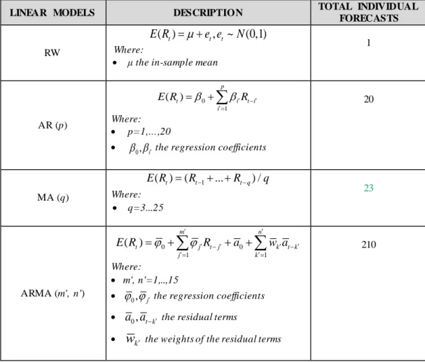
The forecasting ability of the proposed methodology is evaluated over a feature space that is synthesized by individual linear and non-linear forecasts of each exchange rate over the periods outlined in table 2. More specifically, the pool is consisted by a Random Walk (RW), a series of Autoregressive (AR), Moving Average (MA), Autoregressive Moving Average (ARMA) linear models and five non-linear algorithms, namely a Nearest Neighbors Algorithm (k-NN) a Multi-Layer Perceptron (MLP), a Recurrent Neural Network (RNN), a Higher Order Neural Network (HONN) and a Psi-Sigma Neural Network (PSN). A summary of the used linear models is presented in table 4 below, while the applied non-linear models are explained in Appendix B.

Table 4: The summary description of the linear models

LINEAR MODELS DESCRIPTION TOTAL INDIVIDUAL

FORECASTS

RW

( )t t, t ~ (0,1)

E R = +µ e e N

Where:

• μ the in-sample mean

1 AR (p) 0 1 ( ) p t i t i i E R β β_′R_−′ ′= = +

∑

• β β₀, _i′ the regression coefficients

20 MA (q) 1 ( )_t ( _t ... _{t q}) / E R = R₋ + +R₋ q Where: • q=3...25 23 ARMA (m', n') 0 0 1 1 ( ) m n t j t j k t k j k E R j j R a w a ′ ′ ′ − ′ ′ − ′ ′= ′= = +

∑

∑

• j j₀, _j′ the regressioncoefficients • a a₀, t k− ′ the residual terms

• w_k′ the weights of the residual terms

210

These models create a pool of 259 individual forecasts in total for each forecasting exercise. The algorithm genetically searches the above feature space and selects the optimal feature subsets. In all cases, GA selects as inputs for the proposed model among the MLP, HONN, RNN, PSN and k-NN predictors. In other words, the model discards as inputs the linear predictors in favor of the

non-linear models (see table 5). This was expected to some extent due to the non-non-linear nature of the financial time series.

In the final stage of the algorithm, RG-SVR applies a GA to select the SVR parameters. As mentioned before this process is repeated every ten trading days, in order the proposed model capture any possible structural break in the series under study. Although the selection of the inputs seems to be consisted in the majority of the runs for the three exchange rates, this is not the case for the SVR parameters as the C, v and γ parameters vary between 4.10 to 9.20, 0.35 to 0.84 and 8.12 to 19.77 respectively. These variations of the parameters through the different sliding window iterations enable it to adjust to the continuously changing real financial model. It is worth noting that the proposed RG-SVR methodology is fully adaptive. The practitioner does not need to experiment with the parameters of the algorithm in order to optimize the forecasts. RG-SVR structure and its parameters are generated in a single optimization procedure, which prevents the data snooping effect.

4.3 Benchmark Models

The statistical and trading efficiency of the hybrid model is initially evaluated by benchmarking it with traditional genetic and non-genetically optimized SVRs and SVMs. For the non-genetically optimized SVRs, the selection of the inputs and the SVR parameters is optimized with the statistical methods that dominate the relevant literature (grid search or 5-cross validation over the in-sample period)5. The genetically optimized SVR and SVM benchmarks are constructed following the instructions of those introducing them in the literature (see table 1). A summary of the SVR-SVM benchmarks is presented below:

• An ε-SVR model that implements a 5-fold cross-validation and a simple data-driven calculation on the in-sample dataset to calculate parameters ε, γ and C respectively (ε-SVR1).

• A v-SVR model that calculates its parameters v, γ and C as the ε-SVR1 (v-SVR1).

• An ε-SVR and v-SVR model that all parameters are selected based on a grid-search algorithm in the in-sample dataset (ε-SVR2 and v-SVR2).

• A GA-SVM model as proposed by Min et al. (2006), Wu et al. (2007) and Dunis et al. (2013)

• A GA-εSVR model as proposed by Pai et al. (2006), Chen and Wang (2007) and Yuan (2012).

For more on the ε-SVR1 and v-SVR1 approaches see Duan et al. (2003) and Cherkassky and Ma

(2004), while for the ε-SVR2 and v-SVR2 see Schölkopf and Smola (2002).

5

The inputs in all cases of forecasting exercise 1 are selected based on 5-fold cross validation, while in forecasting exercises 2 and 3 with grid search. For the forecasting exercise 4, the inputs selected for EUR/USD and EUR/GBP are based on grid search algorithms, while the ones for EUR/JPY are derived based on 5-fold cross validation.

In addition, Sermpinis et al. (2013) introduce the ARBF-PSO method in a forecasting and trading competition of several linear and non-linear models. Their hybrid NN structure proves to be superior in statistical and trading terms over the more traditional MLP, RNN and PSN. The authors investigate the ECB daily fixings of EUR/USD, EUR/GBP and EUR/JPY over the period of 04/01/1999 to 29/04/2011 (3158 trading days). Their statistical and trading results are not directly comparable with the ones of this study, since their in-sample and out-of-sample periods are overlapping with those of table 2. Nonetheless, ARBF-PSO’s performance is impressive over a dataset of the same three exchange rates that this study is investigating. Thus, ARBF-PSO seems a perfect benchmark for RG-SVR. More details on the ARBF-PSO can be found in appendix B.

The selected inputs for all the benchmark models are presented in the following table.

Table 5: Summary of selected inputs of all models

*Panel A and B include the input selection per each series under study for forecasting exercises 1, 2 and 3, 4 respectively. RG-SVR estimates its inputs every 10 trading days. In other words, in each of the four forecasting exercises RG-SVR algorithm re-estimates its inputs 51 times (the out-of-sample is always between 511 and 516 days). In the table below for the sake of space, we present the three most popular inputs of RG-SVR in each forecasting exercise (RG-SVR(pop)). The minimum numbers of inputs (for all forecasting exercises and re-estimations) selected by the GA for the RG-SVR were 3 and the maximum 5.

PANEL A 1 2

EUR/USD EUR/GBP EUR/JPY EUR/USD EUR/GBP EUR/JPY

ARBF-PSO MLP, HONN, _{RNN, PSN} MLP, HONN, _{RNN, PSN RNN,PSN,} MLP, HONN, _k-NN MLP, HONN, _{RNN,PSN RNN, PSN,} MLP, HONN, _k-NN MLP, HONN, _{RNN, PSN}

ε-SVR1 MLP, HONN, RNN, PSN, k-NN MLP, RNN, PSN, k-NN MLP, HONN, RNN, PSN, k-NN RNN, PSN, k-NN MLP, HONN, RNN, PSN, k-NN MLP, RNN, PSN, k-NN ε-SVR2 MLP, HONN, RNN, PSN, k-NN MLP, HONN, RNN MLP, HONN, RNN, PSN HONN, RNN, PSN, k-NN MLP, HONN, RNN, PSN MLP, HONN, RNN, PSN, k-NN

v-SVR1 MLP, HONN, _{RNN, PSN RNN, PSN, k-NN} MLP, HONN, _{RNN, PSN,} MLP, HONN, _{k-NN RNN, PSN,} MLP, HONN, _k-NN HONN, RNN, _{PSN, k-NN} MLP, HONN, _{RNN, PSN}

v-SVR2 MLP, HONN, RNN _{RNN, PSN,} MLP, HONN, _{k-NN RNN, PSN,} MLP, HONN, _k-NN MLP, RNN, _{PSN, k-NN} MLP, HONN, _{RNN,PSN RNN, PSN,} MLP, HONN, _k-NN

GA-SVM _{RNN, PSN,} MLP, HONN, _k-NN MLP, HONN, _{RNN, PSN} MLP, , RNN, _{PSN, k-NN RNN, PSN,} MLP, HONN, _{k-NN RNN, PSN,} MLP, HONN, _{k-NN RNN, PSN,} MLP, HONN, _k-NN

GA-εSVR MLP, HONN, RNN, PSN, k-NN RNN, PSN, k-NN MLP, HONN, RNN, PSN, k-NN MLP, HONN, RNN, k-NN MLP, HONN, RNN, PSN, k-NN HONN, RNN, PSN, k-NN RG-SVR (pop) MLP, HONN, RNN MLP, RNN, k-NN MLP, HONN, RNN MLP, HONN, RNN MLP, HONN, RNN MLP, RNN, PSN PANEL B 3 4

EUR/USD EUR/GBP EUR/JPY EUR/USD EUR/GBP EUR/JPY

ARBF-PSO _{RNN, PSN,} MLP, HONN, _{k-NN RNN, PSN,} MLP, HONN, _k-NN MLP, HONN, _{PSN, k-NN} MLP, HONN, RNN MLP, HONN, _{PSN, k-NN} MLP, RNN, _{PSN, k-NN}

ε-SVR1 MLP, HONN, _{RNN, PSN} MLP, HONN, RNN, _{PSN, k-NN RNN, PSN,} MLP, HONN, _{k-NN RNN, PSN,} MLP, HONN, _{k-NN RNN, PSN,} MLP, HONN, _k-NN MLP, RNN, _{PSN, k-NN}

ε-SVR2 MLP, HONN, RNN, PSN MLP, HONN, RNN, PSN MLP, HONN, RNN, PSN, k-NN HONN, RNN, PSN, k-NN MLP, HONN, RNN, PSN MLP, HONN, RNN, PSN, k-NN v-SVR1 MLP, HONN, RNN, PSN, k-NN MLP, HONN, RNN, PSN, k-NN MLP, HONN, RNN, PSN, k-NN HONN, RNN, PSN, k-NN MLP, HONN, RNN, PSN MLP, HONN, RNN, PSN v-SVR2 HONN, RNN, PSN, k-NN MLP, HONN, RNN, PSN, k-NN MLP, RNN, PSN, k-NN MLP, HONN, RNN, PSN, k-NN MLP, HONN, RNN, PSN, k-NN MLP, HONN, RNN, PSN, k-NN GA-SVM MLP, HONN, _{RNN, PSN} MLP, HONN, _{RNN, PSN} MLP, HONN, _{PSN, k-NN} HONN, RNN, _{PSN, k-NN RNN, PSN,} MLP, HONN, _{k-NN RNN, PSN,} MLP, HONN, _k-NN

GA-εSVR MLP, HONN, RNN, k-NN MLP, HONN, RNN, PSN, k-NN MLP, HONN, RNN, PSN, k-NN MLP, HONN, RNN MLP, HONN, RNN, PSN MLP, HONN, RNN, PSN, k-NN RG-SVR

(pop) MLP, HONN, PSN HONN, RNN, k-NN

MLP, RNN,

PSN MLP, HONN, RNN MLP, HONN, RNN HONN, RNN, PSN

It is notable that all models apply non-linear predictors as inputs. The five non-linear predictors seem to contain all the information that the two hundred fifty four linear ones contain. This was expected to some extent by the non-linear behavior of financial trading series such as the ones under study.

5. STATISTICAL PERFORMANCE

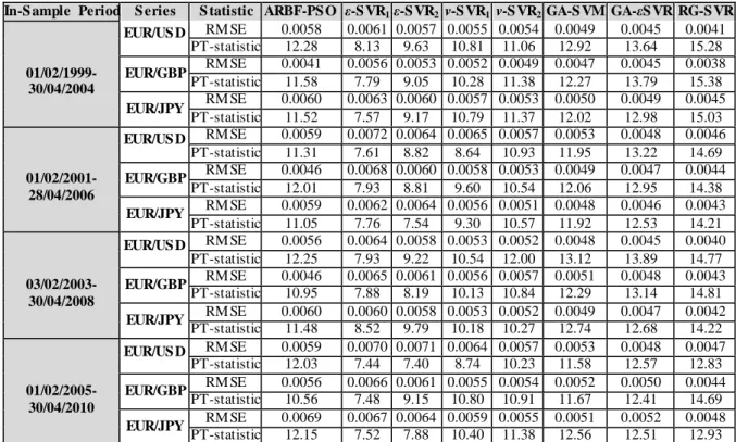
As it is standard in the literature, in order to evaluate statistically the obtained forecasts, the Root Mean Squared Error (RMSE) is computed. The mathematical formula of this statistic is presented in Appendix C. The lower the output the better the forecasting accuracy of the model concerned. The Pesaran-Timmermann (PT) test (1992) examines whether the directional movements of the real and forecast values are in step with one another. In other words, it checks how well rises and falls in the forecasted value follow the actual rises and falls of the time series. The null hypothesis is that the model under study has no power on forecasting the relevant exchange rate. The in-sample statistical performance of the models for the four forecasting exercises and the EUR/USD, EUR/GBP and EUR/JPY exchange rates is presented in table 6 below.

Table 6: Summary of In-Sample Statistical Performance

The results of table 6 show that RG-SVR presents the best in-sample statistical performance for every exchange rate under study. The PT-statistics rejects the null hypothesis of no forecasting power at the 1% confidence interval for all models and series under study. It is also notable that the v-SVR models (v-SVR1 and v-SVR2) have lower RMSEs of the statistical measures than the ε-SVR ones (ε

-SVR1 and ε-SVR2). Additionally the genetically optimized models clearly outperform their statistical

optimized SVR benchmarks. ARBF-PSO presents occasionally better RMSE values than some SVR-In-S ample Period S eries S tatistic ARBF-PS O ε-SVR1ε-SVR2 v-S VR1 v-S VR2 GA-S VM GA-εSVR RG-SVR

01/02/1999- 30/04/2004 EUR/US D RM SE 0.0058 0.0061 0.0057 0.0055 0.0054 0.0049 0.0045 0.0041 PT-statistic 12.28 8.13 9.63 10.81 11.06 12.92 13.64 15.28 EUR/GBP RM SE 0.0041 0.0056 0.0053 0.0052 0.0049 0.0047 0.0045 0.0038 PT-statistic 11.58 7.79 9.05 10.28 11.38 12.27 13.79 15.38 EUR/JPY RM SE 0.0060 0.0063 0.0060 0.0057 0.0053 0.0050 0.0049 0.0045 PT-statistic 11.52 7.57 9.17 10.79 11.37 12.02 12.98 15.03 01/02/2001- 28/04/2006 EUR/US D RM SE 0.0059 0.0072 0.0064 0.0065 0.0057 0.0053 0.0048 0.0046 PT-statistic 11.31 7.61 8.82 8.64 10.93 11.95 13.22 14.69 EUR/GBP RM SE 0.0046 0.0068 0.0060 0.0058 0.0053 0.0049 0.0047 0.0044 PT-statistic 12.01 7.93 8.81 9.60 10.54 12.06 12.95 14.38 EUR/JPY RM SE 0.0059 0.0062 0.0064 0.0056 0.0051 0.0048 0.0046 0.0043 PT-statistic 11.05 7.76 7.54 9.30 10.57 11.92 12.53 14.21 03/02/2003- 30/04/2008 EUR/US D RM SE 0.0056 0.0064 0.0058 0.0053 0.0052 0.0048 0.0045 0.0040 PT-statistic 12.25 7.93 9.22 10.54 12.00 13.12 13.89 14.77 EUR/GBP RM SE 0.0046 0.0065 0.0061 0.0056 0.0057 0.0051 0.0048 0.0043 PT-statistic 10.95 7.88 8.19 10.13 10.84 12.29 13.14 14.81 EUR/JPY RM SE 0.0060 0.0060 0.0058 0.0053 0.0052 0.0049 0.0047 0.0042 PT-statistic 11.48 8.52 9.79 10.18 10.27 12.74 12.68 14.22 01/02/2005- 30/04/2010 EUR/US D RM SE 0.0059 0.0070 0.0071 0.0064 0.0057 0.0053 0.0048 0.0047 PT-statistic 12.03 7.44 7.40 8.74 10.23 11.58 12.57 12.83 EUR/GBP RM SE 0.0056 0.0066 0.0061 0.0055 0.0054 0.0052 0.0050 0.0044 PT-statistic 10.56 7.48 9.15 10.80 10.91 11.67 12.41 14.69 EUR/JPY RM SE 0.0069 0.0067 0.0064 0.0059 0.0055 0.0051 0.0052 0.0048 PT-statistic 12.15 7.52 7.88 10.40 11.38 12.56 12.51 12.93

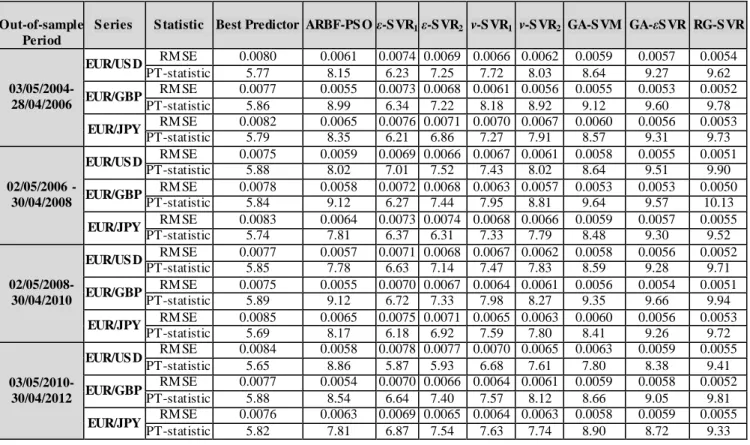
SVM benchmarks, but it always underperforms in comparison to RG-SVR. Table 7 summarizes the statistical performance of the models under study in the out-of-sample period. As a reference, the overall performance of the best predictor is presented in the first column (see Appendix D).

Table 7: Out-Of-Sample Statistical Performance

Out-of-sample Period

S eries S tatistic Best Predictor ARBF-PS O ε-SVR1ε-SVR2 v-S VR1 v-S VR2 GA-S VM GA-εSVR RG-SVR

03/05/2004- 28/04/2006 EUR/US D RM SE 0.0080 0.0061 0.0074 0.0069 0.0066 0.0062 0.0059 0.0057 0.0054 PT-statistic 5.77 8.15 6.23 7.25 7.72 8.03 8.64 9.27 9.62 EUR/GBP RM SE 0.0077 0.0055 0.0073 0.0068 0.0061 0.0056 0.0055 0.0053 0.0052 PT-statistic 5.86 8.99 6.34 7.22 8.18 8.92 9.12 9.60 9.78 EUR/JPY RM SE 0.0082 0.0065 0.0076 0.0071 0.0070 0.0067 0.0060 0.0056 0.0053 PT-statistic 5.79 8.35 6.21 6.86 7.27 7.91 8.57 9.31 9.73 02/05/2006 - 30/04/2008 EUR/US D RM SE 0.0075 0.0059 0.0069 0.0066 0.0067 0.0061 0.0058 0.0055 0.0051 PT-statistic 5.88 8.02 7.01 7.52 7.43 8.02 8.64 9.51 9.90 EUR/GBP RM SE 0.0078 0.0058 0.0072 0.0068 0.0063 0.0057 0.0053 0.0053 0.0050 PT-statistic 5.84 9.12 6.27 7.44 7.95 8.81 9.64 9.57 10.13 EUR/JPY RM SE 0.0083 0.0064 0.0073 0.0074 0.0068 0.0066 0.0059 0.0057 0.0055 PT-statistic 5.74 7.81 6.37 6.31 7.33 7.79 8.48 9.30 9.52 02/05/2008- 30/04/2010 EUR/US D RM SE 0.0077 0.0057 0.0071 0.0068 0.0067 0.0062 0.0058 0.0056 0.0052 PT-statistic 5.85 7.78 6.63 7.14 7.47 7.83 8.59 9.28 9.71 EUR/GBP RM SE 0.0075 0.0055 0.0070 0.0067 0.0064 0.0061 0.0056 0.0054 0.0051 PT-statistic 5.89 9.12 6.72 7.33 7.98 8.27 9.35 9.66 9.94 EUR/JPY RM SE 0.0085 0.0065 0.0075 0.0071 0.0065 0.0063 0.0060 0.0056 0.0053 PT-statistic 5.69 8.17 6.18 6.92 7.59 7.80 8.41 9.26 9.72 03/05/2010- 30/04/2012 EUR/US D RM SE 0.0084 0.0058 0.0078 0.0077 0.0070 0.0065 0.0063 0.0059 0.0055 PT-statistic 5.65 8.86 5.87 5.93 6.68 7.61 7.80 8.38 9.41 EUR/GBP RM SE 0.0077 0.0054 0.0070 0.0066 0.0064 0.0061 0.0059 0.0058 0.0052 PT-statistic 5.88 8.54 6.64 7.40 7.57 8.12 8.66 9.05 9.81 EUR/JPY RM SE 0.0076 0.0063 0.0069 0.0065 0.0064 0.0063 0.0058 0.0059 0.0055 PT-statistic 5.82 7.81 6.87 7.54 7.63 7.74 8.90 8.72 9.33

From table 7 it is suggested that RG-SVR retains its forecasting superiority in the out-of-sample period. The genetically optimized SVRs and SVMs outperform their statistically optimized benchmarks while the PT-statistics indicate that all models continue to forecast accurately the directional change of the three exchange rates. In the out-of-sample statistical evaluation, ARBF-PSO still remains less efficient than the proposed model, although in most cases it outperforms the traditional SVR in terms of RMSE. Tables 5 and 6 show that the grid-search optimized SVRs outperform their counterparts optimized with 5-cross validation while the v-SVR models produce more accurate forecasts that the ε-SVR algorithms. The results support the arguments of Yuan (2012) on the performance of the GA-εSVR over the traditional SVR models.

In order to further verify the statistical superiority of the proposed algorithm, the Diebold-Mariano (DM) (1995) statistic for predictive accuracy is computed, while the MSE is considered as the loss function. The test is applied in the four consecutive out-of-sample periods. Table 8 below presents the DM statistic comparing the RG-SVR with its benchmarks.

Table 8: Diebold-Mariano statistic for each exchange rate under study

Period Best Predictor ARBF-PS O ε-SVR1 ε-SVR2 v-S VR1 v-S VR2 GA-S VM GA-εSVR

U R / U S D 28/04/2006 02/05/2006 - 30/04/2008 -6.90 -3.86 -6.14 -5.20 -5.74 -4.75 -3.46 -3.13 02/05/2008- 30/04/2010 -7.05 -3.91 -5.88 -5.42 -5.01 -4.77 -4.01 -3.72 03/05/2010- 30/04/2012 -7.47 -3.94 -5.63 -5.84 -5.15 -4.89 -4.35 -4.16 E U R / G B P 03/05/2004- 28/04/2006 -6.72 -3.75 -5.47 -5.39 -5.06 -4.53 -3.84 -3.58 02/05/2006 - 30/04/2008 -7.14 -3.87 -5.42 -5.11 -4.88 -4.46 -3.69 -3.22 02/05/2008- 30/04/2010 -6.81 -3.96 -5.79 -5.62 -5.35 -4.92 -3.57 -3.42 03/05/2010- 30/04/2012 -6.92 -3.99 -5.74 -5.23 -4.84 -4.56 -3.88 -3.60 E U R / J P Y 03/05/2004- 28/04/2006 -7.23 -4.25 -6.49 -6.10 -5.71 -5.39 -4.18 -4.05 02/05/2006 - 30/04/2008 -7.56 -4.63 -6.12 -6.45 -5.22 -4.75 -4.51 -4.10 02/05/2008- 30/04/2010 -7.61 -4.07 -6.57 -6.19 -5.70 -5.15 -3.73 -3.51 03/05/2010- 30/04/2012 -7.18 -4.12 -5.88 -5.51 -4.95 -4.67 -3.75 -3.94

From the above table it is obvious that the null hypothesis of equal predictive accuracy is rejected for all comparisons and for both loss functions at the 1% confidence interval (absolute values higher than the critical value of 2.33). Moreover, the statistical superiority of RG-SVR forecasts is confirmed as the realizations of the DM statistic are negative6.

6. TRADING PERFOMANCE

Section 5 evaluates the forecasts through a series of statistical accuracy measures and tests. However, statistical accuracy is not always synonymous with financial profitability. In financial applications, the practitioner’s utmost interest is to produce models that can be translated to profitable trades. It is therefore crucial to further examine the proposed model and evaluate its utility through a trading strategy. The trading strategy applied is to go or stay ‘long’ when the forecast return is above zero and go or stay ‘short’ when the forecast return is below zero. The ‘long’ and ‘short’ EUR/USD, EUR/GBP or EUR/JPY position is defined as buying and selling Euros at the current price respectively. Therefore, the trigger for taking a position is the sign of the daily obtained forecast.

In order to calculate transaction costs, trading positions are needed. Transaction costs for a tradable amount, say USD 5-10 million, are about 1 pip per trade (one way) between market makers. But since the EUR/USD, EUR/GBP and EUR/JPY time series are considered as a series of middle rates, the transaction cost is one spread per round trip. For this dataset a cost of 1 pip is equivalent to an average cost of 0.0074%, 0.0117% and 0.0091% per position for the EUR/USD, the EUR/GBP and the EUR/JPY respectively. The annualized return after transaction costs is simply the annualized

6

In this study, we apply the DM test to couples of forecasts (RG-SVR vs. another forecasting model). A negative realization of the DM test statistic indicates that the first forecast (RG-SVR) is more accurate than the second forecast. The lower the negative value, the more accurate are theRG-SVR forecasts.

return minus the relevant annualized transaction cost. The annualized transaction cost is the annualized number of transactions multiplied with their relevant cost. Table 9 presents the summary of the in-sample trading performance of the models for each exchange rate under study, while Appendix C includes the specification of the trading performance measures used in this paper.

Table 9: Summary of In-Sample Trading Performance

In-S ample Period S eries S tatistic ARBF-PS O ε-SVR1 ε-SVR2 v-S VR1 v-S VR2 GA-S VM GA-εSVR RG-SVR

01/02/1999- 30/04/2004 EUR/US D Annualized Return (including costs) 25.95% 18.25% 19.99% 22.13% 22.81% 25.77% 28.20% 32.92% Information Ratio (including costs) 2.41 1.69 1.85 2.01 2.09 2.34 2.59 2.99 Maximum Drawdown -20.11% -11.12% -12.11% -11.33% -12.92% -13.45% -12.53% -12.74% EUR/GBP Annualized Return (including costs) 28.44% 19.94% 20.18% 21.70% 23.29% 25.62% 27.91% 29.57% Information Ratio (including costs) 2.62 1.81 1.83 1.97 2.12 2.31 2.53 2.69 Maximum Drawdown -14.55% -13.96% -13.58% -12.61% -12.84% -12.28% -12.56% 12.16% EUR/JPY Annualized Return (including costs) 27.07% 21.45% 21.62% 22.47% 22.93% 27.12% 28.38% 30.65% Information Ratio (including costs) 2.32 1.96 1.99 2.07 2.11 2.48 2. 64 2.74 Maximum Drawdown -21.57% -12.84% 13.46% -12.05% -12.88% -12.01% -12.17% -11.93% 01/02/2001- 28/04/2006 EUR/US D Annualized Return (including costs) 23.14% 20.53% 22.77% 21.84% 22.98% 25.80% 27.64% 30.04% Information Ratio (including costs) 2.25 1.88 2.08 1.97 2.11 2.35 2.53 2.77 Maximum Drawdown -21.35% -13.17% -12.55% -12.26% -14.61% -12.10% -12.04% -12.11% EUR/GBP Annualized Return (including costs) 30.55% 22.79% 24.06% 26.56% 27.85% 29.14% 31.02% 33.43% Information Ratio (including costs) 2.78 2.05 2.18 2.39 2.53 2.62 2.81 3.04 Maximum Drawdown 15.39% -14.23% -13.79% -13.32% -14.47% -13.01% -13.94% -13.29% EUR/JPY Annualized Return (including costs) 30.44% 24.71% 24.98% 25.57% 27.99% 28.61% 30.48% 32.80% Information Ratio (including costs) 2.76 2.27 2.29 2.34 2.55 2.60 2.79 2.99 Maximum Drawdown -19.05% -13.47% -14.91% -13.03% -14.52% -15.11% -13.18% -13.48% 03/02/2003-30/04/2008 EUR/US D Annualized Return (including costs) 30.11% 23.57% 25.66% 27.83% 28.90% 31.29% 32.78% 33.16% Information Ratio (including costs) 2.87 2.19 2.40 2.57 2.68 2.92 3.04 3.09 Maximum Drawdown -23.59% -14.08% -14.72% -14.05% -13.49% -13.63% -14.81% -14.38% EUR/GBP Annualized Return (including costs) 28.33% 22.06% 23.61% 24.40% 25.77% 27.83% 27.58% 29.45% Information Ratio (including costs) 2.67 2.07 2.21 2.28 2.42 2.61 2.59 2.76 Maximum Drawdown -15.92% -13.75% -14.42% -13.40% -14.09% -14.45% -14.16% -14.21% EUR/JPY Annualized Return (including costs) 30.90% 23.92% 24.58% 26.61% 27.84% 29.15% 31.77% 32.36% Information Ratio (including costs) 2.79 2.14 2.20 2.37 2.49 2.61 2.84 2.91 Maximum Drawdown -18.55% -14.42% -14.68% -14.26% -14.17% -14.85% -14.51% -14.63% 01/02/2005- 30/04/2010 EUR/US D Annualized Return (including costs) 31.05% 20.49% 21.03% 25.37% 27.72% 30.51% 32.00% 33.46% Information Ratio (including costs) 2.84 1.88 1.92 2.33 2.53 2.79 2.93 3.07 Maximum Drawdown -24.17% -17.91% -18.46% -17.05% -17.88% -17.60% -18.59% -17.96% EUR/GBP Annualized Return (including costs) 30.87% 22.96% 24.85% 27.54% 27.16% 29.83% 31.48% 33.20% Information Ratio (including costs) 2.89 2.14 2.28 2.56 2.53 2.78 2.93 3.10 Maximum Drawdown -17.25% -17.49% -17.22% -17.95% -17.20% -17.51% -17.72% -17.38% EUR/JPY Annualized Return

Information Ratio

(including costs) 1.86 1.92 2.08 2.17 2.34 2.68 2.79 3.04 Maximum Drawdown -20.15% -17.74% -18.53% -18.86% -18.02% -18.22% -18.84% -18.49%

From the results of the above table, RG-SVR demonstrates superior trading performance in terms of annualized return and information ratio for all exchange rates and in-sample periods. The maximum drawdowns of the benchmark models are worse than the RG-SVR ones. Their trading performance in the out-of-sample period is presented in table 10 below.

Table 10: Summary of Out-of-Sample Trading Performance

Out-of-S ample

Period S eries S tatistic

Best

Predictor ARBF-PS O ε-SVR1 ε-SVR2 v-S VR1 v-S VR2 GA-S VM GA-εSVR RG-SVR

03/05/2004- 28/04/2006 EUR/US D Annualized Return (including costs) 8.17% 20.05% 10.44% 11.06% 15.87% 17.81% 19.90% 20.65% 24.77% Information Ratio (including costs) 0.76 1.85 0.96 1.02 1.46 1.64 1.83 1.90 2.34 Maximum Drawdown -15.26% -15.03% -14.09% -14.42% -13.01% -13.65% -12.41% -12.69% -12.84% EUR/GBP Annualized Return (including costs) 10.39% 19.87% 12.21% 14.55% 15.40% 16.92% 18.79% 20.26% 22.04% Information Ratio (including costs) 1.04 1.91 1.22 1.47 1.54 1.69 1.89 2.03 2.27 Maximum Drawdown -14.36% -10.85% -14.60% -13.85% -13.88% -13.93% -13.86% -13.10% -13.28% EUR/JPY Annualized Return (including costs) 9.08% 18.56% 10.96% 12.47% 15.91% 16.53% 19.39% 20.20% 23.65% Information Ratio (including costs) 0.83 1.67 0.99 1.13 1.43 1.50 1.75 1.82 2.13 Maximum Drawdown -15.82% -13.92% -14.19% -14.52% -14.39% -14.01% -13.62% -13.40% -13.81% 02/05/2006 - 30/04/2008 EUR/US D Annualized Return (including costs) 8.83% 18.92% 10.29% 13.04% 12.85% 14.47% 18.37% 19.86% 22.19% Information Ratio (including costs) 0.81 1.71 0.94 1.19 1.17 1.32 1.67 1.80 2.02 Maximum Drawdown -15.53% -14.58% -14.39% -14.23% -13.99% -13.44% -14.61% -14.70% -14.57% EUR/GBP Annualized Return (including costs) 10.10% 20.38% 13.64% 15.58% 16.75% 18.16% 20.14% 21.08% 24.61% Information Ratio (including costs) 1.12 2.24 1.49 1.70 1.83 1.98 2.21 2.28 2.79 Maximum Drawdown -16.82% -11.03% -15.61% -15.29% -14.58% -14.33% -14.89% -14.48% -14.84% EUR/JPY Annualized Return (including costs) 9.29% 19.04% 12.22% 12.83% 14.80% 15.32% 18.41% 19.62% 22.47% Information Ratio (including costs) 0.81 1.63 1.06 1.11 1.28 1.33 1.58 1.69 1.93 Maximum Drawdown -15.93% -13.14% -15.30% -15.46% -15.04% -15.53% -15.62% -15.45% -15.24% 02/05/2008-30/04/2010 EUR/US D Annualized Return (including costs) 10.68% 23.15% 12.25% 14.72% 16.50% 19.00% 21.12% 22.95% 24.71% Information Ratio (including costs) 1.07 2.34 1.23 1.47 1.66 1.89 2.11 2.30 2.49 Maximum Drawdown -15.29% -10.23% -14.08% -14.15% -14.06% -13.48% -13.63% -14.85% -14.30% EUR/GBP Annualized Return (including costs) 8.59% 20.15% 10.06% 12.61% 13.24% 14.97% 18.34% 19.01% 20.65% Information Ratio (including costs) 1.05 2.32 1.18 1.49 1.55 1.76 2.16 2.21 2.44 Maximum Drawdown -16.11% -11.47% -15.19% -15.51% -15.70% -14.84% -14.29% -15.02% -15.31% EUR/JPY Annualized Return (including costs) 8.74% 23.19% 12.03% 13.35% 16.42% 17.56% 20.02% 22.87% 24.96% Information Ratio (including costs) 0.70 1.89 0.97 1.08 1.33 1.42 1.63 1.86 2.02 Maximum Drawdown -15.18% -9.17% -15.58% -15.32% -16.00% -15.82% -14.73% -14.92% -15.02% 03/05/2010- 30/04/2012 EUR/US D Annualized Return (including costs) 9.54% 21.56% 11.63% 12.48% 15.12% 16.69% 19.09% 20.60% 23.41% Information Ratio (including costs) 0.86 1.95 1.06 1.15 1.39 1.50 1.75 1.90 2.14 Maximum Drawdown -16.77% -9.32% -16.20% -16.27% -15.84% -16.49% -15.35% -15.58% -15.64% EUR/GBP Annualized Return

Information Ratio (including costs) 1.06 2.59 1.40 1.42 1.73 1.69 2.09 2.37 2.71 Maximum Drawdown -18.52% -12.93% -18.06% -17.17% -17.95% -17.63% -17.22% -17.53% -17.39% EUR/JPY Annualized Return (including costs) 8.37% 20.35% 10.25% 11.82% 12.48% 14.02% 17.43% 18.12% 22.08% Information Ratio (including costs) 0.68 1.62 0.79 0.96 1.03 1.15 1.42 1.48 1.80 Maximum Drawdown -14.49% -10.74% -14.81% -14.74% -15.01% -14.36% -14.57% -14.23% -14.40%

RG-SVR continues to outperform all other SVR forecast combination models in terms of trading efficiency. GA-εSVR is found to be the second best model in forecasting exercises 1 and 2. RG-SVR presents on average 3% higher annualized returns and 0.33 higher information ratios compared to GA-εSVR in these first two simulations. In the other two exercises the results of ARBF-PSO are better than GA-εSVR, which is ranked third. RG-SVR again achieves higher profits and information ratios than ARBF-PSO on an average of 1.46% and 0.15 respectively. Thus, the proposed methodology clearly outperforms its benchmarks in terms of statistical accuracy and financial profitability. The non-genetically optimized SVR methodologies remain less efficient in trading terms compared to their counterparts. But it is interesting to outline the profitability divergence between the different SVR models. For instance, between v-SVR2 and ε-SVR1 there is an average

difference of 4.55% in annualized returns after transaction costs for the three exchange rates. Smaller differences are also evident in the other SVR approaches. The SVR’s trading performance appears very sensitive to the parameters optimization process.

7. CONCLUDING REMARKS

The motivation of this paper is to introduce a RG-SVR model for optimal parameter selection and feature subset combination, when applied to the task of forecasting and trading the EUR/USD, EUR/GBP and EUR/JPY exchange rates. The proposed model genetically searches over a pool of individual forecasts, identifies the optimal feature subsets and finally provides a robust single SVR forecast combination for each exchange rate. This is achieved by applying a fitness function specialized for financial purposes and adopting a sliding window approach. RG-SVR is benchmarked not only against genetically and non-genetically optimized SVRs, but also a robust hybrid NN, the ARBF-PSO.

RG-SVR presents the best performance in terms of statistical accuracy and trading efficiency for all the exchange rates under study. RG-SVR’s superiority not only confirms the success of the implemented fitness function, but also validates the benefits of applying GAs to v-SVR models. The results also support prior evidence of ARBF-PSO’s efficiency in forecasting and trading the three exchange rates. ARBF-PSO outperforms in all simulations the traditional SVRs. RG-SVR is far more profitable, though. The large differences in the trading performance of the models under study,

indicates the sensitivity of SVRs to their parameters optimization processes. In summary, the empirical evidence provided by this study should go some way towards convincing statisticians and practitioners to experiment beyond the bounds of traditional SVR optimization techniques.

REFERENCES

BASAK, D., PAL, S. & PATRANABIS, D. C. (2007) Support Vector Regression, Neural Information Processing - Letters and Reviews, 11 (10), pp. 203-224.

CAO, L.J., CHUA, K.S. & GUAN, L.K. (2003) C-ascending support vector machines for financial time series forecasting, IEEE International Conference on Computational Intelligence for Financial Engineering Proceedings, pp. 317-323.

CHERKASSKY, V. & MA, Y. (2004) Practical selection of SVM parameters and noise estimation for SVM regression, Neural Networks, 17 (1), pp. 113-126.

CHEN, K.Y. & WANG, C.H. (2007) Support Vector Regression with genetic algorithms in forecasting tourism demand, Tourism Management, 28 (1), pp. 215-226.

DIEBOLD, F.X. & MARIANO, R.S. (1995) Comparing Predictive Accuracy, Journal of Business and Economic Statistics, 20(1), pp. 134-144.

DUAN, K., KEERTHI, S.S. & POO, A.N. (2003) Evaluation of simple performance measures for tuning SVM hyperparameters, Neurocomputing, 51, pp. 41-59.

DUNIS, C.L., LAWS, J. & SERMPINIS, G. (2010) Modeling and Trading the EUR/USD Exchange Rate at the ECB fixing, The European Journal of Finance, 16 (6), pp. 541-560.

DUNIS, C.L., LAWS, J. & SERMPINIS, G. (2011) Higher order and recurrent neural architectures for trading the EUR/USD exchange rate, Quantitative Finance, 11 (4), pp. 615-629.

DUNIS, C.L., LIKOTHANASSIS, S.D., KARATHANASOPOULOS, A.S., SERMPINIS, G. & THEOFILATOS, K.A. (2013) A hybrid genetic algorithm–support vector machine approach in the task of forecasting and trading, Journal of Asset Management, 14(1), pp. 52-71.

DUNIS, C.L. & NATHANI, A. (2007) Quantitative Trading of Gold and Silver using Non-linear Models, Neural Network World, 16 (2), pp. 93-111.

ELMAN, J.L. (1990) Finding structure in time, Cognitive Science, 14 (2), pp. 179-211.

FISMAN, R. (2001) Estimating the Value of Political Connections, The American Economic Review, 91(4), pp. 1095-1102.

FIX, E. & HODGES, J.L. (1951) Discriminatory analysis, nonparametric discrimination: Consistency properties. Technical Report 4, USAF School of Aviation Medicine, Randolph Field, Texas.

FROOT, K.A., SCHAFRSTEIN, D.S. & STEIN, J.C. (1992) Herd on the street: Informational inefficiencies in a market with short-term speculation, Journal of Finance, 47 (4), pp. 1461–1484. GENG, R., BOSE, I. & CHEN, X. (2015) Prediction of financial distress: An empirical study of listed Chinese companies using data mining, European Journal of Operational Research, 241 (1), pp. 236-247.

GHOSH, J. & SHIN, Y. (1991) The Pi-Sigma Network: An efficient Higher-order Neural Networks for Pattern Classification and Function Approximation, Proceedings of International Joint Conference of Neural Networks, 1, pp. 13-18.

HOLLAND, J. (1975) Adaptation in Natural and Artificial Systems: An Introductory Analysis with Applications to Biology, Control and Artificial Intelligence, Cambridge, Mass: MIT Press.

HUCK, N. & GUÉGAN, D. (2005) On the Use of Nearest Neighbors to Forecast in Finance, Revue de l'Association française de Finance, 26, pp.67-86.

HSU, S.H., HSIEH, J. J. P.A., CHIH, T.C. & HSU, K.C. (2009) A two-stage architecture for stock price forecasting by integrating self-organizing map and support vector regression, Expert Systems with Applications, 36(4), pp. 7947-7951.

HUANG, S.C., CHUANG, P.J., WU, C.F. & LAI, H.J. (2010) Chaos-based support vector regressions for exchange rate forecasting, Expert Systems with Applications, 37(12),pp. 8590-8598.