A fast pulse phase estimation method for X-ray
pulsar signals based on epoch folding
Xue Mengfan, Li Xiaoping
*, Sun Haifeng, Fang Haiyan
School of Aerospace Science and Technology, Xidian University, Xi’an 710126, China Received 26 July 2015; revised 3 December 2015; accepted 1 February 2016 Available online 10 May 2016
KEYWORDS Epoch folding; Maximum likelihood; Phase estimation; X-ray pulsar; X-ray pulsar-based navigation (XPNAV)
Abstract X-ray pulsar-based navigation (XPNAV) is an attractive method for autonomous deep-space navigation in the future. The pulse phase estimation is a key task in XPNAV and its accuracy directly determines the navigation accuracy. State-of-the-art pulse phase estimation techniques either suffer from poor estimation accuracy, or involve the maximization of generally non-convex object function, thus resulting in a large computational cost. In this paper, a fast pulse phase estimation method based on epoch folding is presented. The statistical properties of the observed profile obtained through epoch folding are developed. Based on this, we recognize the joint prob-ability distribution of the observed profile as the likelihood function and utilize a fast Fourier transform-based procedure to estimate the pulse phase. Computational complexity of the proposed estimator is analyzed as well. Experimental results show that the proposed estimator significantly outperforms the currently used cross-correlation (CC) and nonlinear least squares (NLS) estima-tors, while significantly reduces the computational complexity compared with NLS and maximum likelihood (ML) estimators.
Ó2016 Production and hosting by Elsevier Ltd. on behalf of Chinese Society of Aeronautics and Astronautics. This is an open access article under the CC BY-NC-ND license (http://creativecommons.org/ licenses/by-nc-nd/4.0/).
1. Introduction
Pulsars are highly magnetized, rapidly rotating neutron stars emitting uniquely identifiable signals that are periodical and predictable, throughout the electromagnetic spectrum with periods ranging from milliseconds to thousands of seconds.
The repetition period of the radiation signals is simply the rotation period of the neutron star. For some pulsars, the sta-bility of their rotation periods over long timescales is as precise as an atomic clock.1–3Of all pulsars, the ones which are visible in the X-ray band of the electromagnetic spectrum are called ‘‘X-ray pulsar”.3,4Compared with the other types of pulsars, the X-ray pulsars are more suitable for use in deep space nav-igation because of the existence of small size X-ray detectors that can be mounted on a spacecraft.5
X-ray pulsar-based navigation (XPNAV) is a developing celestial navigation method and receives increasing attention. It is promising to fulfill completely autonomous navigation to reduce the dependence of current navigation system to ground-based operations, or to argument the current systems * Corresponding author. Tel.: +86 29 81891036.
E-mail address:[email protected](X. Li).
Peer review under responsibility of Editorial Committee of CJA.
Production and hosting by Elsevier
Chinese Journal of Aeronautics, (2016),29(3): 746–753
Chinese Society of Aeronautics and Astronautics
& Beihang University
Chinese Journal of Aeronautics
[email protected]www.sciencedirect.com
http://dx.doi.org/10.1016/j.cja.2016.03.005
1000-9361Ó2016 Production and hosting by Elsevier Ltd. on behalf of Chinese Society of Aeronautics and Astronautics. This is an open access article under the CC BY-NC-ND license (http://creativecommons.org/licenses/by-nc-nd/4.0/).
by employing additional measurements to improve their per-formance.4–7The concept of employing X-ray pulsars to esti-mate the position of deep space explorer was first proposed in 1974 and has grew rapidly during the last 40 years.8United States and the European Space Agency have analyzed the fea-sibility of XPNAV and continuously studied on the subject.9–12 In the recent years, many researchers have investigated dif-ferent applications of NPNAV, including both absolute and relative navigations.13–15It has been shown that one key issue of XPNAV is how to precisely estimate the phase delay between the observed profile and the predicted one.13–16 To date, many pulse phase estimation algorithms have been devel-oped for XPNAV. The maximum likelihood (ML) phase esti-mator presented in Ref.13directly utilizes the detected photon time of arrivals (TOAs); its estimation accuracy approaches the Crame´r-Rao lower bound (CRLB) as the observation duration increases, but the direct employment of the photon TOAs makes the amount of calculation and storage rapidly increase with the growth of received photons and the direct search of the ML solution also leads to a high computational cost. The Fourier transform-based pulse delay estimation method given by Taylor has the advantage that its accuracy is independent of the bin size, but it inevitably involves a straightforward iterative procedure which is computationally intensive.17Emadzadeh has proposed two different pulse delay estimators based on the observed profile obtained through epoch folding.4,13One uses the cross-correlation (CC) function between the photon intensities and greatly reduces the compu-tational cost compared with the ML estimator. The other is a nonlinear least squares (NLS) estimator. However, both esti-mators suffer from poor estimation accuracy and are not asymptotically efficient, and the NLS estimator still involves the maximization of a non-convex objective function, thus resulting in a direct search-based procedure. In Ref.18, the authors describe an approximate ML estimator at low signal to noise ratio (SNR) values. The appropriate approximation of the likelihood function reduces the computational complex-ity, but results in a degradation of the estimation accuracy as the SNR values increase due to the deviation between the established statistical model of the observed profile and the exact situation. In Ref.19, the authors recast the problem of pulsar phase estimation as a cyclic shift parameter estimation problem under multinomial distributed observations and develop a fast near-maximum likelihood phase estimation method based on this. This strategy is essentially based on the conditional probability density function of the photon TOA and actually complicates the phase estimation problem of X-ray pulsar, which can be directly mathematically formu-lated by the epoch folding procedure as presented in the subse-quent content of this paper.
In this paper, the X-ray pulsar radiation is characterized as a non-homogeneous Poisson process (NHPP) and the observed profile obtained through the epoch folding procedure is statistically modeled as a heteroscedastic Poisson sequence. Upon this model, we recognize the joint probability distribu-tion of the observed profile as the likelihood funcdistribu-tion and employ a computationally efficient fast Fourier transform (FFT) based procedure to estimate the pulse phase of X-ray pulsar signals. The rest of this paper is organized as follows. In Section 2, the mathematical models describing the X-ray pulsar signals are presented. Based on this, the heteroscedastic Poisson model formulating the observed profile is established.
Section3explains how the pulse phase can be estimated by a FFT based procedure by employing the joint probability distri-bution of the observed profile as the likelihood function. Com-putational complexity of the proposed estimator is studied in Section4. In Section5, experiments are carried out to evaluate this new technique’s performance, using both simulated data and real data. Finally, Section6concludes the study.
2. Heteroscedastic Poisson model of X-ray pulsar observed profile
The original measurement of X-ray pulsar is the TOAs of all the X-ray photons from the pulsar source as well as the back-ground. TOA of a photon is recorded by the X-ray detector when the photon hits the detecting material.20–22In XPNAV, a low power X-ray detection system capable of measuring the photon TOAs with submicro second accuracy is required. The detector must have a low background noise, a large detec-tion area and a light weight. The Naval Research Laboratory (NRL), as part of the Defense Advanced Research Projects Agency (DARPA), has developed a new X-ray silicon-based detector that satisfies all the above-mentioned requirements.19 To obtain the observed profile, the measured photon TOAs are first transformed to the solar system barycenter (SSB) and then assembled into a single pulse cycle through the procedure of epoch folding.3–5,13In this paper, to focus our discussion, we assume that the photon TOAs have been transformed to SSB. In what follows, according to the presented X-ray detec-tion method, mathematical equadetec-tions are used to describe the photon TOAs at the SSB; then upon this, statistical properties of the observed profile are given.
2.1. Mathematical model of X-ray pulsar signals
LetNt be the number of arrival photons at the time interval ð0;tÞ. The counting processfNðtÞ;tP0gcan be modeled by a NHPP with a time-varying intensitykðtÞP0.23,24For a fixed time intervalðts;teÞ, the number of arrival photonsNts;te is a Poisson random variable with parameterRtstekðtÞdt. Its distri-bution low is PðNts;te¼kÞ ¼ Rte ts kðtÞdt k exp RtstekðtÞdt k! ð1Þ
and its mean and variance are EðNts;teÞ ¼varðNts;teÞ ¼
Rte
ts kðtÞdt ð2Þ
Furthermore, since fNðtÞ;tP0g has independent incre-ments, the numbers of detected photons in any non-overlapping time intervals are independent from each other. The intensity functionkðtÞwhose unit is ph/s includes all the arriving photons from the X-ray pulsar and the background. It is expressed as
kðtÞ ¼aþbhð/ðtÞÞ ð3Þ
wherehð/Þis the normalized pulsar profile,/ðtÞrepresents the evolution of the pulse phase with respect to the timetas seen at the SSB, andaandbare the known effective background and source photon arrival rates, respectively. The pulsar profile hð/Þ, which is unique to a particular pulsar and defines the
non-homogeneous nature of the source photons, is defined at the phase interval ½0;1Þ and normalized to satisfy min/2½0;1Þhð/Þ ¼0 and R01hð/Þd/¼1, and then its definition
domain is extended beyond ½0;1Þ by letting hð/þnÞ ¼ hð/Þ 8n2Z.23,24Fig. 1shows the profile of the Crab pulsar (PSR B0531+21) in the X-ray band (2–16 keV), created by using about 1000 s real data observed by the rossi X-ray timing explorer (RXTE).
The pulse phase/(t) is the sum of the initial phase/0at a
reference timet0and the accumulation of phase sincet0. It can
be expressed as the Taylor series
/ðtÞ ¼/0þfðtt0Þ þ _ f 2ðtt0Þ 2þ OðmÞ ð4Þ
where f and f_are the X-ray source frequency and its first derivative valid at timet0, respectively, andOðmÞis the
high-order item and is expressed as OðmÞ ¼X M m¼2 fðmÞðtt0Þ m m! ð5Þ
with fðmÞ the mth derivation of the source frequency at time
t0.23 The parameters f, f_and fðmÞ of a pulsar are obtained
through pulsar timing techniques and they need to be con-stantly revised to minimize the pulsar timing residuals which would result in additional uncertainties of the pulse phase. For example, the abovementioned Crab pulsar is the brightest rotation-powered pulsar in the X-ray band, yielding about 9.9109ergs/(cm2/s) of X-ray energy flux in the 2–10 keV band, which is a significant advantage for its application in spacecraft navigation,3but it is also a young pulsar and its tim-ing residuals exhibit significant timtim-ing noise, so its phase model needs to be frequently revised to minimize the timing noise and optimal extrapolation of its timing residuals is essential for it to be used in navigation.25,26
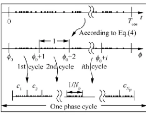
2.2. Epoch folding
The process of epoch folding is to recover the observed profile from the photon TOAs.3–5,13,23,24It is implemented as follows: All the time tags within an observation are folded back into one phase cycle of the source by calculating their correspond-ing phase values accordcorrespond-ing to the phase model of Eq.(4)and then only retaining the fractional part of each phase value, which is referred to as the normalized phase. Afterwards, divide the phase cycleð0;1Þ into some equal-length bins and
drop each of the normalized phase values into the appropriate phase bin. The resulting histogram over one phase cycle is the so-called observed profile of X-ray pulsar. The overall epoch folding procedure is illustrated inFig. 2.
Assume that the observation duration is Tobs, one phase
cycle contains Nb bins, and ci denotes the photon count of the ith bin after the epoch folding procedure. According to Eqs.(1) and (2),ciis a Poisson random variable with the fol-lowing mean and variance:
EðciÞ ¼varðciÞ ¼ Tobs Nb kpð/iÞ ð6Þ where kpð/iÞ ¼aþbhð/iÞ ð7Þ
/i is the center phase of theith bin and/i¼/0þi=Nb. It is
shown that the variance ofci changes with the phase. There-fore, the observed profile, denoted by fcig
Nb
i¼1, can be
mathe-matically formulated by a heteroscedastic Poisson model. Moreover, according to the independent increment property of the Poisson process,ciis statistically uncorrelated, namely, EðcjckÞ ¼EðcjÞEðckÞ ð8Þ
3. Fast maximum likelihood phase estimator
After the observed profilefcigNbi¼1 is derived through the epoch
folding procedure described in Section 2.2, employing the Nb-dimensional joint probability distribution of the observed
profile, a maximum likelihood phase estimation problem can be formulated to estimate the unknown initial phase/0.
According to Eq. (6), the probability distribution of the random variableciis Pðcij/0Þ ¼ ðkpð/iÞTobs=NbÞ ciexpðk pð/iÞTobs=NbÞ ci! ð9Þ
Additionally, sinceci is statistically uncorrelated, the joint probability distribution of the observed profile is multinomial and is given by PðfcigNbi¼1j/0Þ ¼ YNb i¼1 Pðcij/0Þ ¼Y Nb i¼1 ðkpð/iÞTobs=NbÞ ciexpðk pð/iÞTobs=NbÞ ci! ð10Þ Recognizing the joint probability distribution given in Eq. (10) as the likelihood function, an ML estimator based on
Fig. 1 Profile of Crab pulsar obtained by RXTE.
the observed profile is provided by maximizing Eq.(10)with respect to the unknown parameter /0. Equivalently, the log-likelihood function (LLF) can be maximized. It is expressed as LLFð/0Þ ¼ABþ XNb i¼1 ci ln½kpð/0þi=NbÞ ð11Þ where A¼lnY Nb i¼1 ðTobs=NbÞci ci! B¼Tobs Nb XNb i¼1 kpð/0þi=NbÞ 8 > > > > < > > > > : ð12Þ
It is obvious that the term A does not depend on the unknown parameter/0. Furthermore, sincekpð/Þis a periodic
function, its integral sum over one period is not a function of the initial phase/0, which means that the termBis also
inde-pendent of/0. Therefore, the termAandBcan be dropped from the LLF. We end up with the following LLF:
LLFð/0Þ ¼
XNb i¼1
ciln½kpð/0þi=NbÞ ð13Þ
The initial phase can be estimated by solving the following optimization problem: ^ /0¼arg max /02½0;1Þ XNb i¼1 ciln½kpð/0þi=NbÞ ð14Þ
Then we define u^0¼1/^0. According to the periodicity of kpð/Þ, the following estimation rule is obtained:
^ u0¼arg max u02ð0;1 XNb i¼1 ciln½kpði=Nbu0Þ ð15Þ
After defining ^k¼ ½ciNbi¼1 and kðu0Þ ¼ ½ln½kpði=Nbu0Þ
Nb i¼1,
Eq.(15)can be expressed as ^ u0¼arg max u02ð0;1 ^ kTkðu 0Þ ð16Þ
Since the statistickðu0Þis a periodic function, the inner
multi-plication on the right-hand side of Eq.(16)can be recognized as the cyclic CC function between the observed profile^kand the logarithmic transformation of the actual radiation intensity as a function ofu0.
In order to exploit the cyclic convolution property of the FFT for the evaluation of the global maximum of Eq. (16), we discretize the rangeð0;1of the parameteru0intoNb
inter-vals of width 1=Nb. The indexku, corresponding to a coarse estimate u^c
0 of u0 with a resolution of 1=Nb, namely
^
uc
0¼ku=Nb, can be obtained from(16)rewritten as27
ku¼arg max k
^
kTDkkð0Þ ð17Þ
whereDis the following orthogonal unit matrix27:
D¼ 0 0 1 1 0 ... .. . 0 0 1 0 .. . 0 ... ... ... .. . ... 0 0 1 0 2 6 6 6 6 6 6 6 6 4 3 7 7 7 7 7 7 7 7 5 ð18Þ
The objective sequencef¼ ½^kTDkkð
0ÞNbk¼1can be calculated by using the FFT of both^kandkð0Þ.27Specifically, the FFT of the observed profile^kis computed and multiplied by the com-plex conjugated FFT of the zero phase-offset intensity sequence kð0Þ so as to obtain their cyclic cross correlation sequencefafter the inverse FFT.
Since the resolution of the coarse estimateu^c
0 provided by
the discrete cross correlation is definitely limited by the value ofNb, a fine estimate u^0 is attained by means of a parabolic
interpolation of the objective sequencefaround its maximum fðkuÞ.
Moreover, it is interesting to notice that the estimation rule Eq.(15) is close to the CC estimator,4 from which it differs mainly by the employment of the logarithm ofkpð/Þinstead
ofkpð/Þ. Actually, since the logarithmic transformation is a
kind of variance stabilizing transformations,28it can, to some extent, eliminate the influence of the heteroscedastic property of the observed profile described in Section2.2on the phase estimation accuracy. Therefore, our proposed estimator may have a higher precision compared with the CC estimator. This is also validated by the experimental results presented in Section5.
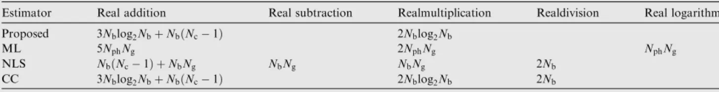
4. Computational complexity analysis
In this section, the computational complexity of the proposed pulse phase estimator is studied and is compared with that of the currently used estimators. Since when considering the change in the source frequency, the procedure of transforming the photon TOAs into photon phases based on the phase model Eq.(4)is needed for all the phase estimators, in the fol-lowing comparison analysis we assume the phase values of all the arrival photons have been known for the sake of simplicity. To use the proposed estimator, the observed profile is needed. To obtain it,NbðNc1Þreal additions must be
per-formed, withNcbeing the number of phase cycles within the
observation time. Since the computed photon counts need not to be normalized in our epoch folding procedure, the 2Nbdivisions needed in the epoch folding procedure given in
Refs.23,24 can be eliminated. Since the
Nb real logarithms
needed to construct the cost function can be pre-calculated, we do not contain this part of calculation into the computa-tional cost of the proposed estimator. To calculate the cyclic cross-correlation sequence in the cost function Eq.(17), two Nb-point FFT and aNb-point inverse FFT are involved, which
requires a total number of 2Nblog2Nbreal multiplications and
3Nblog2Nbreal additions, assuming that one complex addition
contains two real additions and one complex multiplication contains four real multiplications and two real additions. Hence, the total operations required by the proposed estimator are approximately 3Nblog2NbþNbðNc1Þreal additions and
2Nblog2Nbreal multiplications. We observe that the amount of
necessary additions is a linear function ofNc and grows
lin-early as the observation time increases, and the required real multiplications only depend on the number of bins in one phase cycle,Nb.
We also give the computational complexities of state of the art phase estimators to perform a contrastive analysis. The ML estimator derived in Ref.13 needs a total number of 5NphNg
logarithms, where Nph denotes the total number of detected
photons within the observation duration. Note that the amount of calculations is proportional to the number of received photons and it will significantly increase as the obser-vation time becomes longer, which is a noticeable defect of the ML method. The NLS estimator presented in Refs.13,17,24 requiresNbðNc1Þreal additions and 2Nbreal divisions for
the epoch folding procedure andNbNg real additions, NbNg
real multiplications and NbNg real subtractions for the grid
search, withNg being the number of grid points considered.
The CC estimator developed in Ref.4requires the same opera-tions as the NLS estimator to implement the epoch folding procedure and the same operations as the proposed estimator to calculate the cyclic CC sequence.
A comparison of the complexities of all the methods men-tioned above is summarized inTable 1. It is worth noting that sinceNphNb in most cases, the computational cost of the
ML is the highest. Taking the Crab pulsar as an example, when the detector area is 200 cm2, approximately 9105 photons could be detected within an observation duration of 30 s, which corresponds to about 898 phase cycles. SettingNb¼Ng¼1024,
the total numbers of arithmetic operations needed by the ML, NLS and CC methods are about 7.373109, 4.066106and 9.717105, respectively, whereas the proposed estimator only requires about 9.696105operations.
5. Experimental results and discussion
To evaluate the performance of the proposed pulse phase esti-mator, a series of experiments is carried out using both the simulated data obtained by the ground-based simulation sys-tem and the real data obtained by the RXTE satellite. We assess the performance of proposed estimator against the other three methods discussed in Section4, including the ML estima-tor, the NLS estimator and the CC estimator.
5.1. Simulated photon TOAs
5.1.1. Ground-based simulation system of X-ray pulsar signals Fig. 3shows the principle diagram of the X-ray pulsar signal ground-based simulation system, which consists of three
modules: The voltage source module, the optical attenuation module and the photon detection module. The voltage source module with high time–frequency stability is to synthesize a voltage signal of similar shape as the intensity function. It includes an atomic clock, a crystal oscillator, a frequency synthesizer and an arbitrary waveform generator. Under the premise of the physical process being consistent, we replace the X-ray source with the visible light source in order to reduce costs. The optical attenuation module generates the single pho-ton sequence by simulating the practical attenuation process in the propagation of the X-ray signal. In this module, an elec-tronic control visible light source and a variable optical atten-uator are fixed inside an optical shielding cavity. The photon detection module, which includes a photomultiplier, an optical pulse discriminator and the electronic readout circuit, is designed to record the photon TOAs.
With the characteristics of high time resolution of 10 ns, high stability up to 109, low dark counts and small counting error, the simulation system can generate photon TOAs of any known pulsar. For detailed information, you can refer to our previous work.29It is noteworthy that what this system simu-lates is the photon TOAs transformed to the SSB, but not the photon TOAs directly detected by the detector onboard a moving spacecraft, and the system cannot simulate the change in the source frequency yet, meaning that in Eq.(4), the first and higher order derivatives of the source frequency are all set to zero. Since the simplified constant frequency model does not affect the validation of the pulse phase estimation algo-rithms, in the following numerical simulations, we use this sim-ulation system to generate the photon TOAs of the selected pulsars.
5.1.2. Results and analyses
Two pulsars are selected: B0531+21 (Crab) and B150958, whose simulation parameters are listed inTable 2.4,13The sim-ulation results are obtained by using the Monte-Carlo tech-nique, with 100 independent realizations of photon time tags generated by the ground-based simulation system. The initial phase/0 is set to be 0.3021. The number of bins in one pulse cycle, namely Nb, is set as 1024 for Crab and 512 for
B150958. The number of grid points Ng of the NLS and Table 1 Computational costs of different estimators.
Estimator Real addition Real subtraction Realmultiplication Realdivision Real logarithm Proposed 3Nblog2NbþNbðNc1Þ 2Nblog2Nb
ML 5NphNg 2NphNg NphNg
NLS NbðNc1Þ þNbNg NbNg NbNg 2Nb
CC 3Nblog2NbþNbðNc1Þ 2Nblog2Nb 2Nb
ML estimators is set equal toNbso as to ensure the same phase
resolution as the CC and the proposed estimator. For a fair comparison, the procedure of parabolic interpolation of the cost function around its maximum is also employed in the ML, NLS and CC methods to obtain a fine estimate. We eval-uate the estimation accuracy in terms of root mean square error (RMSE), which is defined as
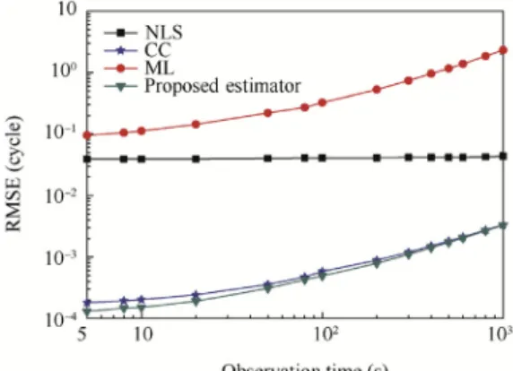
RMSEð/^0Þ ¼ ffiffiffiffiffiffiffiffiffiffiffiffiffiffiffiffiffiffiffiffiffiffiffiffiffi Eð/^0/0Þ 2 q ð19Þ In the first scenario, giving a fixed SNR value, we test the estimators’ performance for different observation times using Crab pulsar. InFig. 4, the RMSE of the four methods for each observation time is plotted against the square root of the CRLB calculated according to Ref.13, at a background arrival ratea¼4:4 ph=ðcm2=sÞ, corresponding to SNR 10 dB. It
can be seen that when the observation time is short, a relatively large deviation between the RMSE and the square root of the CRLB is introduced no matter what estimator is used. The rea-son is that for a short observation time, the realization of the photon TOAs is not enough to represent the intensity function precisely, leading to a cost function whose global optimum generally locates at a farther point to the true value, u0. As time goes on, the RMSE of each method becomes more attached to the CRLB and approaches to zero, also indicating that the proposed estimator is consistent. Besides, simulation results show that the proposed estimator outperforms the NLS and CC estimators and keeps close to the ML estimator at almost all the observation times. This is due to the fact that the established heteroscedastic Poisson model can accurately formulate the observed profiles of any observation times.
As a second scenario, we evaluate the RMSE versus SNR. The pulsar B150958 is considered. We fix the observation time at 300 s and calculate the RMSE of each estimator at dif-ferent SNR values varying from23 dB to 32 dB. The obser-vation time is set to be 300 s. Simulation results plotted in Fig. 5 show that when the SNR is less than 5 dB, the
proposed estimator performs only slightly better than the NLS and CC estimators, whereas as the SNR grows higher, the proposed estimator tends to have more and more obvious advantage than the NLS and CC estimators. When the SNR is higher than 5 dB, the NLS and CC estimators enter into the saturation region, with their RMSE values changeless with the increasing SNR values, while the proposed estimator still keeps tightly attached to the ML estimator and clearly outper-forms the NLS and CC estimators.
Although the ML estimator has an advantage over the pro-posed estimator on the estimation accuracy, the operation time taken by the estimator should be taken into consideration. In Fig. 6, the CPU time cost by MATLAB to implement the cal-culation for one Monte-Carlo realization is plotted as a func-tion of the observafunc-tion time. The processor utilized is an Intel 2.5 GHz dual core. It can be seen that the CPU time for the ML estimator is much bigger than the ones for the other esti-mators, especially the CC and the proposed estiesti-mators, and it linearly grows as the observation time becomes longer and grows significantly faster than the other three estimators. The NLS, CC and the proposed estimators all totally contain two procedures, namely the epoch folding and the construction of cost function, of which the CPU time for the former grows linearly with the observation time and the CPU time for the latter does not change with the observation time, leading to linearly growing in these three estimators’ computational com-plexities with the observation time. Because the cost function construction time for the NLS estimator is bigger than the
Table 2 Parameters of employed pulsars. Pulsar Period (s) Source flux
(2–10 keV) ph/(cm2/s)
Detector area (cm2)
B0531+21 0.0334 1.54 100
B150958 0.1502 1.62102 2000
Fig. 4 RMSE of different estimators for Crab.
Fig. 5 RMSE versus SNR for B1509-58 atTobs¼300 s.
ones for the CC and the proposed estimators and the time costs of the epoch folding procedure are almost the same for the three estimators, both CC and the proposed estimators require much lower computational load than the NLS estima-tor, especially when the observation time is short, as is shown in Fig. 6, which is consistent with the results discussed in Section4. Furthermore, the proposed estimator costs slightly less time than the CC estimator due to the elimination of the 2Nbreal divisions in the epoch folding procedure.
5.2. Real data from RXTE
We use real data of the Crab pulsar obtained with the propor-tional counter array (PCA) on board RXTE. The PCA, which is a low-energy (2–60 keV) detection instrument, consists of five xenon-filled proportional counter units (PCUs) with a total effective area of about 6500 cm2. Its time resolution is 1ls. We perform the data extraction and the profile generation using the RXTE standard data analysis software, FTOOLS 4.0.30 The event mode data of the observation 96802-01-12-00 detected in MJD 55776 is selected. To identify periods of good data from the whole observation duration, the following selection criteria are applied.30
(1) The minutes since the peak of the last South Atlantic Abnormal passage are larger than 30.
(2) The pointing offset of the detector is less than 0.02°. (3) The electron contamination of each PCU is smaller than
0.1.
(4) To avoid contamination due to Earth’s X-ray bright limb, the elevation angle of the source above the space-craft horizon must be greater than 10°.
After filtering out the band timespan, all the reserved time tags are first transformed to the SSB to eliminate the Doppler effect, in which process the various clock corrections, the Roe-mer delay and the relativistic effects including the Sun Shapiro and the Einstein delays are considered,30and then the trans-formed time tags are folded back into one phase cycle to gen-erate the observed profile. The above two steps are implemented by employing the ‘Fasebin’ and ‘Fbssum’ opera-tions, of whichNbis set to 1024. The observed profiles of the
delayed version are generated by directly adding a delay of 9 ms, corresponding to an initial phase of 0.2674, into the cor-rected time tags before epoch folding. We take the observed profile obtained over the total left exposure time of about 1011 s as the reference profile to be compared with the delayed profile. The background and the source arrival rates are about 8.813103ph/s and 1:0216103ph=s, respectively, corre-sponding to SNR 10 dB.
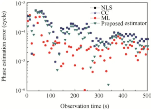
Fig. 7shows the phase estimation errors of the four meth-ods for different observation times. The proposed estimator outperforms the NLS and CC estimators at most observation times, especially when the observation time is long, and its esti-mation accuracies keep close to the ones of the ML method at most observation times that are longer than 350 s, which is consistent with the simulation results given in Section5.1. It is noteworthy that since the source arrival rate is large, when the observation time is long, the phase estimation accuracy is limited by the time resolution of the detected time tags and does not present a notable improvement, as can be seen in
Fig. 7. The fluctuation occurring between 350 s and 400 s may be caused by a kind of unknown strong noise during this period of observation.
6. Conclusions
This paper has presented a new computationally efficient phase estimator for the X-ray pulsar signals. According to the statistical properties of X-ray pulsar signals, a heteroscedastic Poisson model is established to formulate the observed pulsar profile obtained through epoch folding. Based on this model, a new pulse phase estimator which employs the joint probability distribution of the observed profile as the like-lihood function and can be calculated by a FFT-based proce-dure is derived. The performance of the proposed estimator is evaluated by the simulated photon TOAs as well as the real data captured by the RXTE. It is shown that when the obser-vation time is short, our estimator has an estimation accuracy slightly superior to the ones of the NLS and CC estimators, while when the observation time is long, it performs signifi-cantly better than the NLS and CC estimators. Furthermore, its computational cost is much smaller than the ones of the ML and NLS estimators, making the estimator more suitable to be used on the resource-limited spacecraft.
Acknowledgement
This study was supported by the National Natural Science Foundation of China (No. 61301173).
References
1. Matsakis DN, Taylor JH, Eubanks TM, Marshall T. A statistic for describing pulsar and clock stabilities. Astron Astrophys 1997;326(3):924–8.
2. Rots AH, Jahoda K, Lyne AG. Absolute timing of the Crab pulsar with ROSSI X-ray timing explorer.Astrophys J2004;605
(2):L129–32.
3. Sheikh SI. The use of variable celestial X-ray sources for spacecraft navigation dissertation. Maryland: University of Mary-land; 2005.
4. Emadzadeh AA. Relative navigation between two spacecraft using X-ray pulsars dissertation. Los Angeles: University of California; 2009.
Fig. 7 Phase estimation errors of different estimators derived by using real data of Crab.
5. Liu J, Kang ZW, White P. Doppler/XNAV-integrated navigation system using small-area X-ray sensor. IET Radar Sonar Navig 2011;5(9):1010–7.
6. Feng DZ, Xu LP, Zhang H, Song SB. Determination of inter-satellite relative position using X-ray pulsars.J Zhejiang Univ Sci C2013;14(2):133–42.
7. Xue MF, Li XP, Fu LZ, Fang HY, Sun HF, Shen LR. X-ray pulsar-based navigation using pulse phase and Doppler frequency measurements.Sci China Inf Sci2015;58(12) 122202:1-10. 8. Fei BJ, Yao GZ, Du J, Sun WJ. The pulse profile and united
measurement equation in XNAV. Sci China Phys Mech Astron 2011;40(5):644–50.
9. Xue MF, Li XP, Fu LZ, Liu XP, Sun HF, Shen LR. Denoising of X-ray pulsar observed profile in the undecimated wavelet domain. Acta Astronaut2016;118:1–10.
10. Sheikh SI, Pines DJ, Ray PS, Wood KS, Lovellette MN, Wolff MT. Spacecraft navigation using X-ray pulsars. J Guid Control Dyn2006;29(1):49–63.
11. Huang LW, Liang B, Zhang T, Zhang CH. Navigation using binary pulsars.Sci China Phys Mech Astron2012;55(3):527–39. 12. Qiao L, Liu JY, Zheng GL, Xiong Z. Augmentation of XNAV
system to an ultraviolet sensor-based satellite navigation system. IEEE J Sel Top Signal Process2009;3(5):777–85.
13. Emadzadeh AA, Speyer JL. On modeling and pulse phase estimation of X-ray pulsars.IEEE Trans Signal Process2010;58
(9):4484–95.
14. Zhang H, Xu LP. An improved phase measurement method of integrated pulse profile for pulsar.Sci China Technol Sci2011;54
(9):2263–70.
15. Wang YD, Zheng W, Sun SM, Li L. X-ray pulsar-based navigation using time-differenced measurement.Aerosp Sci Tech-nol2014;36:27–35.
16. Liu J, Fang JC, Kang ZW, Wu J, Ning XL. Novel algorithm for X-ray pulsar navigation against Doppler effects. IEEE Trans Aerosp Electron Syst2015;51(1):228–41.
17. Taylor JH. Pulsar timing and relativistic gravity. Philos Trans Phys Sci Eng1992;341(1660):117–34.
18. Li JX, Ke XZ. Maximum-likelihood TOA estimation of X-ray pulsar signals on the basis of Poison model.Chin Astron Astrophys 2011;35(1):19–28.
19. Rinauro S, Colonnese S, Scarano G. Fast near-maximum likeli-hood phase estimation of X-ray pulsars. Signal Process2013;93
(1):326–31.
20. Wang YD, Zheng W, Sun SM. X-ray pulsar-based navigation system/sun measurement integrated navigation method for deep space explorer. Proc IMechE Part G: J Aerosp Eng 2015;229
(10):1842–53.
21. Zhang H, Xu LP, Xie Q. Modeling and Doppler measurement of X-ray pulsar.Sci China Phys Mech Astron2011;54(6):1068–76. 22. Wang YD, Zheng W, Sun SM. X-ray pulsar-based navigation
system with errors in the planetary ephemerides for Earth-orbiting satellite.Adv Space Res2013;51(12):2394–404.
23. Emadzadeh AA, Speyer JL. X-ray pulsar-based relative navigation using epoch folding. IEEE Trans Aerosp Electron Syst2011;47
(4):2317–28.
24. Emadzadeh AA, Jason LS. Relative navigation between two spacecraft using X-ray pulsar.IEEE Trans Control Syst Technol 2011;19(5):1021–35.
25. Deng XP, Coles W, Hobbs G, Keith MJ, Manchester RN, Shannon RM, et al. Optimal interpolation and prediction in pulsar timing.Mon Not R Astron Soc2012;424(1):244–51.
26. Deng XP, Hobbs G, You XP, Li MT, Keith MJ, Shannon RM, et al. Interplanetary spacecraft navigation using pulsars. Adv Space Res2013;52(9):1602–21.
27. Colonnese S, Rinauro S, Scarano G. Generalized method of moments estimation of location parameters: application to blind phase acquisition.IEEE Trans Signal Process2010;58(9):4735–49. 28. Guan Y. Variance stabilizing transformations of Poisson, bino-mial and negative binobino-mial distributions.Stat Probab Lett2009;79
(14):1621–9.
29. Sun HF, Xie K, Li XP, Fang HY, Liu XP, Fu LZ, et al. A simulation technique of X-ray pulsar signals with high timing stability.Acta Phys Sin2013;62(10):109701 Chinese.
30. The ABC of RXTE: Contents Internet. [cited 2015 July 18]. Available from: http://heasarc.gsfc.nasa.gov/docs/xte/abc/con-tents.html/.
Xue Mengfanis a Ph.D. candidate at School of Aerospace Science and Technology, Xidian University. She received the B.S. degree in 2011 from Shijiazhuang Tiedao University. Her research focuses on signal processing theory and X-ray pulsar-based navigation.
Li Xiaopingwas born in 1961. She received her Ph.D. degree from Xidian University in 2004. She is now a professor and Dean of the School of Aerospace Science and Technology of Xidian University. Her research focuses on information fusion, intelligent information processing and information security.
Sun Haifengwas born in 1986. He received his M.S. and Ph.D. degrees from Xidian University respectively in 2011 and 2015. His researches focus on celestial navigation and signal processing theory.