Samoili, Sofia,Bhaskar, Ashish, Hai Pham, Minh, & Dumont, Andre-Gilles (2011) Considering weather in simulation traffic. InThe 11th Swiss
Trans-port Research Conference, 11-13 May 2011, Monte Verita, Ascona.
This file was downloaded from: http://eprints.qut.edu.au/49509/
c
Copyright 2011 [please consult the author]
Notice: Changes introduced as a result of publishing processes such as copy-editing and formatting may not be reflected in this document. For a definitive version of this work, please refer to the published source:
Considering weather in simulating traffic
Sofia Samoili, EPFL
Dr. Ashish Bhaskar, QUT
Minh Hai Pham, EPFL
Prof. André-Gilles Dumont, EPFL
Conference paper STRC 2011
Considering weather in simulating traffic
Sofia Samoili
École Polytechnique Fédérale de Lausanne, School of
Architecture, Civil and Environmental Engineering (ENAC), Laboratory of Traffic
Facilities (LAVOC) Lausanne
Dr. Ashish Bhaskar Queensland University of Technology, School of Urban
Development, Brisbane, Australia
Minh Hai Pham École Polytechnique Fédérale
de Lausanne, School of Architecture, Civil and Environmental Engineering (ENAC), Laboratory of Traffic
Facilities (LAVOC) Lausanne Phone: +41 21 693 06 02 Fax: +41 21 693 63 49 email: [email protected] Phone: +61 731 389 985 Fax: email: [email protected] Phone: +41 21 693 06 03 Fax: +41 21 693 63 49 email: [email protected] Professor André-Gilles Dumont
École Polytechnique Fédérale de Lausanne, School of
Architecture, Civil and Environmental Engineering (ENAC), Laboratory of Traffic
Facilities (LAVOC) Lausanne Phone: +41 21 693 23 89 Fax: +41 21 693 63 49 email: [email protected] 10 February 2011
Abstract
The impact of weather on traffic and its behavior is not well studied in literature primarily due to lack of integrated traffic and weather data. Weather can significant effect the traffic and traffic management measures developed for fine weather might not be optimal for adverse weather.
Simulation is an efficient tool for analyzing traffic management measures even before their actual implementation. Therefore, in order to develop and test traffic management measures for adverse weather condition we need to first analyze the effect of weather on fundamental traffic parameters and thereafter, calibrate the simulation model parameters in order to simulate the traffic under adverse weather conditions.
In this paper we first, analyses the impact of weather on motorway traffic flow and drivers’ behaviour with traffic data from Swiss motorways and weather data from MeteoSuisse. Thereafter, we develop methodology to calibrate a microscopic simulation model with the aim to utilize the simulation model for simulating traffic under adverse weather conditions. Here, study is performed using AIMSUN, a microscopic traffic simulator, though the methodology developed is applicable for any traffic simulation model.
Keywords
1. Introduction
In view of the importance of weather impact on traffic, its behaviour was studied via simulation. This is an efficient tool for analysing traffic management measures even before their actual implementation. Therefore, in order to develop and test traffic management measures for adverse weather condition the effect of weather on fundamental traffic parameters was analysed and thereafter the challenging part of calibrating the simulation model parameters has followed, in order to simulate the traffic under adverse weather conditions. The analytical basis for the simulation model development was formed by the quantification of the relationship between traffic parameters and weather (rainfall) with data from Swiss motorway and meteorological sites. The simulation was performed with a microscopic traffic simulator and the methodology that was developed is applicable for any traffic simulation model.
The analysis of issues that emerge on transportation networks due to adverse weather conditions, the assessment of its impacts and the response to them are to be addressed in the current research. More explicitly the goals of this study are standing on understanding the issues that are related to adverse weather conditions, to assess the impact of weather on traffic, with case study the Swiss motorway network and to respond to the weather by developing traffic management measures under adverse weather conditions. To accomplish these, a modelling of the behaviour of traffic and its dynamics has to be effectuated that in order to be validated as representative with reasonable accuracy, the model parameters had to be calibrated with objective function to minimize the deviation of simulated and observed flow of the network.
2. Methodology
For the traffic simulation of the network a microscopic traffic simulator was used with the following basic structure. Vehicles enter the network entry points and their movements through the network are determined by behavioural models as the car-following, the lane changing and the gap acceptance. A set of vehicle’s and driver’s attributes is assigned to each vehicle, which are used by the behavioural models to model the vehicle movement.
The used simulator can function either as a stochastic model, where vehicles travel through the network based on turn probabilities, or as a traffic assignment model using Origin-Destination tables. In addition, the possibility of considering a dynamic traffic assignment is offered, where optimum vehicle paths between centroids are computed at the beginning of the simulation and then updated based on feedback from the network. Thus, route choice is based on actual traffic conditions and may vary at different points in the simulation.
The input to the simulator includes a simulation scenario and a set of simulation parameters that define the experiment. The scenario is composed of four types of data: network description, traffic control plan, traffic demand data and public transport plans. The simulation parameters are: fixed values, which describe the experiment such as simulation time, warm-up period, statistics interval, etc.; and variable parameters, which are used to calibrate the models such as reaction times, lane changing zone, etc.
The simulator can provide continuous animated graphical representation of traffic network performance, statistical output data (flow, speed, journey times, delays, stops) and data gathered by the simulated detectors (counts, occupancy, speed). In addition, through API access, with which a detailed traffic dynamics is provided during simulation, that can be obtained and controlled as required by the user.
The car-following model that is adopted by the simulator and served as the behavioural model in question, is the Gipps car-following model that considers the vehicle’s speed as the derivative of the displacement and vehicle’s acceleration as the derivative of its speed. In the following section it will be further analysed.
2.1 Simulator’s Car-following Model (Gipps)
The speed during the time t to t+T for a given vehicle n with position x(n,t) is V(n,t+T). Then the position of a vehicle n at time t+T is defined as follows:
( , ) ( , ) ( , )
x n t+T =x n t +V n t+T T
The speed V(n,t+T) at time t+T is defined as the minimum of two speeds Va and Vb as discussed below. The maximum speed Va to which a vehicle n can accelerate during a time period (t, t+T) is given by:
( , ) ( , ) ( , ) ( , ) 2.5 (1 ) 0.025 * ( ) * ( ) a V n t V n t V n t T V n t a T V n V n + = + − +
where: V(n,t) is the speed of the vehicle n at time t,
V*(n) is the desired speed of the vehicle (n) for current section
a(n) is the maximum acceleration for vehicle n and
T is the reaction time.
{
}
2 2 2 ( 1, ) ( , ) ( ) ( ) ( )[2 ( 1, ) ( 1) ( , ) ( , ) '( 1) b V n t V n t T d n T d n T d n x n t s n x n t V n t T d n − + = + − − − − − − − −where: d(n) is the absolute maximum desired deceleration by vehicle n
x(n,t) is the position of vehicle n (follower) at time t
x(n-1,t) is the position of the preceding vehicle (n-1) (leader) at time t
s(n-1) is the effective length of vehicle (n-1)
d’(n-1) is an estimation of vehicle (n-1) desired deceleration.
The relationship between the deceleration of leader and follower is given by the sensitivity factor a as follows
'( 1) * ( 1)
d n− =a d n−
The modeller can also define a minimum headway between vehicles, an additional restriction imposed before the update of the vehicle position. The minimum headway constrain is defined as follows:
[
] [
]
[
]
min min ( 1, ) ( 1) ( , ) ( , ) ( , ). ( ) ( 1, ) ( 1) ( , ) ( ) if x n t T s n x n t V n t T T V n t T h n x n t T s n then V n t T h n T − + − − − + + < + − + − − + = + where: x(n,t) is position of vehicle n at time tx(n-1,t) is position of preceding vehicle (n-1) at time t
s(n-1) is the effective length of vehicle (n-1)
hmin(n) is the minimum headway of vehicle n respect to its follower
Therefore, the parameters of the abovementioned equations that are to be calibrated are: maximum acceleration for vehicle n a(n), reaction time T, maximum deceleration desired by vehicle n d(n), estimation of vehicle (n-1) desired deceleration d’(n-1) and sensitivity factor per vehicle a. These parameters are defined in the vehicle attributes at the level of vehicle type as mean values for the attributes of each vehicle, but also as deviation, maximum and minimum values. The particular characteristics for each vehicle are sampled from a truncated normal distribution and are: length, width, maximum desired speed, maximum acceleration, normal deceleration (maximum deceleration in normal conditions), maximum deceleration (in special circumstances), speed acceptance (degree of acceptance of speed limits), minimum distance between vehicles, maximum give-away time, guidance indications’ acceptance, sensitivity factor, minimum headway (TSS, 2010).
2.2 Validation of the Simulation Model
The reliability of the analysis performed using the simulated data highly depends on the ability of the simulation model to represent traffic and its behaviour with reasonable accuracy.
This ability is usually achieved through the validation process, where the model parameters are calibrated iteratively, with the objective to minimize the deviation of simulated output with the real observation. For instance, the objective can be to minimize the simulated and observed flow on the network:
2 min r s it it i t q q ∀ ∀ −
∑∑
Therefore, the calibration and validation of the simulation models is one of the most challenging and vital part of any simulation model development. The objective of the calibration depends on the application of the developed model.
2.3 Calibration approach and headway distribution fitting
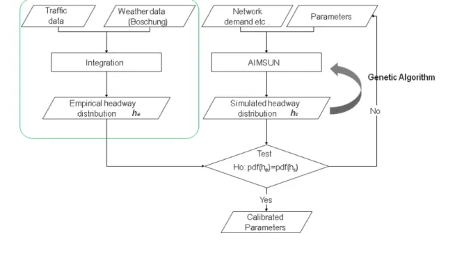
For the current study the focus was set on the calibration of the car-following model in the simulator in question, considering the vehicle headway distribution. The integration of real traffic and weather data provides an empirical headway distribution (he), which will be analysed as follows.
Figure 1 Framework for model calibration
Developed by A. Bhaskar
In order to perform the analysis, the model that was more suitable was the one from Hoogendoorn and Bovy (Hoogendoorn and Bovy, 1998). According to that model, the observed headway h is considered as a random variable from two independent random variables hconstrained and hnonconstrained, that is vehicle headway under constrained and non constrained region respectively. A vehicle is termed as non-constrained when its behaviour is independent of the leading vehicles in the flow and as constrained when its behaviour is determined by the leading vehicle in the flow. The equation that describes the observed headway is the following:
non constrained
* constrained (1 ) * h=θ h + −θ h −
where θ: proportion of constrained vehicle.
Therefore, a car-following behaviour is attributed to the constrained vehicle and its distribution is described by Pearson-III distribution as follows:
( 1) ( ) : 0 ( ) 1 ( ) ( ) w w w w constrained w x d w w w w
h Pearson III distribution
if h d g x h d e if h d β β α α β − − − − < = − ≥ Γ
where Γ is the gamma function, αw and βw are parameters, dw is the minimum headway. A non-constrained vehicle is assumed to have a poisson arrival with negatively exponential headway distribution as follows:
non constrained: ( ) x h Exponentially distributed u x λe λ − − = where λ is the arrival rate.
The density function f(w) defining the distribution of total headway observed at the detector, which is the combination of both constrained and non constrained vehicles, is given as follows: ( ) 0 ( ) * ( ) (1 ) * ( ) * * * w w s f w =θ g w + −θ
∫
g s λ e−λ − d sThe development of the simulation model was performed for the same site, with the demand determined from the detectors of the network. Simulating the model with a set of parameters, the abovementioned car-following parameters, provides the simulated headway distribution (hs) which is then compared with the empirical headway distribution (he). The process is repeated so as to minimize the difference between two distributions. The statistical test to compare the two distributions is the Kolmogorov-Smirnov (KS) test that will be explained in the following section. The value of most of the parameters that are to be calibrated, is bounded with the physical limit of the vehicle and drivers. For instance, vehicle acceleration of 10 m/s2 or drivers reaction time of zero seconds is non-realistic etc. Therefore the
an optimisation technique, genetic algorithm, is adopted in order to converge faster to the set of parameters which minimizes the difference between the observed and simulated headway distribution.
2.4 Kolmogorov-Smirnov (KS) test
Kolmogorov-Smirov (KS) test defines the equality between two continuous probability distributions. The test is non parametric and quantifies the distance between the two cumulative probability distribution functions (pdf). It can be applied to compare a sample (one-sample KS test) with reference probability distribution such as normal, or compare two samples (two-samples KS test).
The two-sample KS test determines if the samples differ significantly by testing the null hypothesis H0 that both the samples are from the same distribution against the alternate hypothesis H1 that the samples are not from the same distribution. It is underlined that this test does not specify the distribution, it only verifies if the two samples are from the common distribution or not. 0 1 1 2 : 1 2 : 1 2
Given datasets D and D
H D and D are from the same distribution H D and D are not from the same distribution
If datasets D1=
{
y y y1, 2, 3,...,yn}
and D2={
z z z1, 2, ,...,3 zm}
have n and m data points represented by variables y and z, respectively, then the functions Fn and Gm represent the cumulative distribution functions for D1 and D2.1 1 ( ) i n n y x i F x I n = ≤ =
∑
1 1 ( ) i m m z x i G x I m = ≤ =∑
Where i z xI ≤ is an indicator function as follows:
1 0 i z x i i I if z x if z x ≤ = ≤ = >
The KS statistic (Dn,m) is defined for the samples as follows:
, su p ( ) ( )
n m x n m
Where supx is the supremum or the Least Upper Bond (LUB), for the set of vertical distances between the two cumulative distribution functions: Fn and Gm.
The null hypothesis Ho is rejected at level α, if:
, n m
nm
D K
n+m > α
3. Results
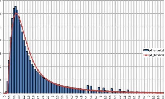
The following figures (Figure 2, Figure 3) illustrate the observed and theoretical (Hoogendoorn and Bovy model) headway distribution at site 149, lanes 1 and 2, for one year (2005) for normal and rainy conditions, respectively.
Figure 2 Probability density function for the empirical and theoretical function for site 149, lane 2 under normal conditions
0 0.01 0.02 0.03 0.04 0.05 0.06 0.07 0 0.3 0.6 0.9 1.2 1.5 1.8 2.1 42. 2.7 3 3.3 3.6 3.9 4.2 4.5 4.8 5.1 5.4 5.7 6 6.3 6.6 6.9 7.2 57. 7.8 8.1 8.4 8.7 9 9.3 9.6 9.9 pdf Headway range pdf_emperical pdf_theoritical
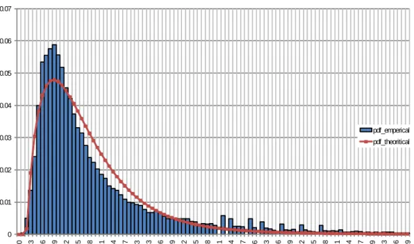
Figure 3 Probability density function for the empirical and theoretical function for site 149, lane 2 under rainy conditions
0 0.01 0.02 0.03 0.04 0.05 0.06 0.07 0 0.3 0.6 0.9 1.2 1.5 1.8 2.1 2.4 2.7 3 3.3 3.6 3.9 4.2 4.5 4.8 5.1 5.4 5.7 6 6.3 6.6 6.9 7.2 7.5 7.8 8.1 8.4 8.7 9 9.3 9.6 9.9 pdf Headway range pdf_emperical pdf_theoritical
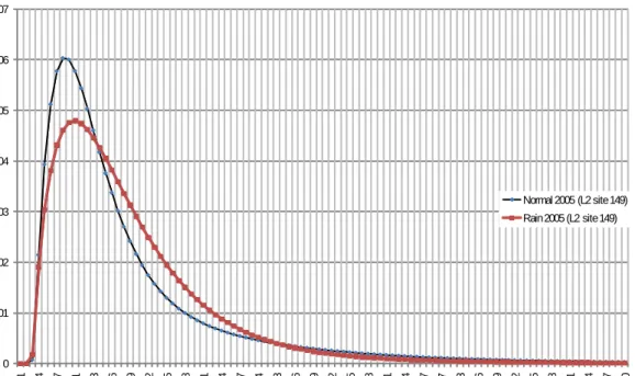
The following figures illustrate the difference between normal and rainy weather based on theoretical (Hoogendoorn and Bovy model) and empirical headway distribution, respectively. As observed at the graph, the rainy conditions result to a headway increase and peak shifts from 0.8 seconds to 1 second with increase in proportion of vehicles with larger headway under rainy conditions. This is in compliance to the expected, theoretical, behaviour, since rainy conditions lower the skid resistance and drivers need to maintain larger headway for safe driving.
Figure 4 Theoretical probability density function for normal and rainy conditions for site 149, lane 2. 0 0.01 0.02 0.03 0.04 0.05 0.06 0.07 0. 1 0.4 0.7 1 1.3 1.6 1.9 2.2 52. 2.8 3.1 3.4 3.7 4 4.3 4.6 4.9 5.2 5.5 5.8 6.1 6.4 6.7 7 7.3 67. 7.9 8.2 8.5 8.8 9.1 9.4 9.7 10 pdf Headway range Normal 2005 (L2 site 149) Rain 2005 (L2 site 149)
Figure 5 Empirical probability density for normal and rainy conditions for site 149, lane 2. 0 0.01 0.02 0.03 0.04 0.05 0.06 0.07 0 0.3 0.6 0.9 1.2 1.5 1.8 2.1 42. 2.7 3 3.3 3.6 3.9 4.2 4.5 4.8 5.1 5.4 5.7 6 6.3 6.6 6.9 7.2 57. 7.8 8.1 8.4 8.7 9 9.3 9.6 9.9 pdf Headway range Normal 2005 (L2 site 149) Rain 2005 (L2 site 149)
4. Perspectives
Following the calibration of the aforementioned traffic behavioural model, a sensitivity analysis could ensue, in terms of unveiling the important parameters, so as to verify the robustness of the simulation model with a different set of parameters and further with greater study area. Among the future plans lies the validation of the calibration of the global microscopic model, such as the gap acceptance, lane-changing models, avoiding the overfitting effect that would render the model incapable of adapting to various networks and situations.
5. References
TSS-Transport Simulation Systems S.L. 2010. Microsimulator and Mesosimulator Aimsun User’s Manual. 25-29, 273-278 p.
Hoogendoorn, S. & Bovy, P. 1998. New Estimation Technique for Vehicle-Type-Specific Headway Distributions. Transportation Research Record: Journal of the Transportation Research Board (TRB), 1646, 18-28 p.