Crypto
currencies’ Internal and External
Relations
A Descriptive Analysis of Cryptocurrency Dynamics and Relations to the US Equity Market
Abstract
This thesis is a descriptive statistical analysis of cryptocurrency market and its relation within cryptocurrencies and across asset classes, using correlation functions, orthogonalized impulse response functions and OLS regressions. Consistent with Wang (2014), bitcoin does not suffer from a liquidity trap, even though bitcoin is a decentralized system. This thesis concludes that bitcoin has a lead effect on only 2 out of 8 of the top cryptocurrencies, endowing diversification benefits within cryptocurrency market. This paper provides evidence on cryptocurrency market’s and US equity market’s impulse response dynamics which are insignificant, consistent with Gangwal’s (2016) results that adding cryptocurrencies to a diversified portfolio will yield to a higher Sharpe ratio. Lastly, the study reports bitcoin momentum factor having an impact on banking and financial industries’ excess returns.
Keywords:
Bitcoin, Bitcoin Liquidity, Bitcoin and Equity Market, Cryptocurrency, Descriptive Analysis, Asset Class, Market Relations
Name: Aleksi Aaltonen Student Number: 481713 Type: Bachelor’s Thesis
Topic: Finance Date: 05.12.2017
2
Contents
1. INTRODUCTION ... 3
2. LITERATURE REVIEW AND HYPOTHESES ... 4
2.1CRYPTOCURRENCIES AS MEANS OF EXCHANGE AND BITCOIN’S LIQUIDITY ... 5
2.2CRYPTOCURRENCIES AS AN ASSET CLASS ... 6
2.2HYPOTHESES ... 7
3. DATA ... 8
3.1CRYPTOCURRENCY DATA & MARKET PROXY ... 8
3.2SAMPLE & DATA GENERATING PROCESS ... 9
4. METHODOLOGY ... 10
4.1ACF,PACF&CCF ... 11
4.2VAR(P) MODEL &ORTHOGONALIZED IMPULSE RESPONSE FUNCTION ... 12
4.3OLS REGRESSION FOR CRYPTOCURRENCY AND MARKET RELATIONS ... 13
5. RESULTS FROM THE STATISTICAL ANALYSIS AND REGRESSIONS ... 14
5.1ORTHOGONALIZED IMPULSE RESPONSE FUNCTIONS ... 14
5.2OLS REGRESSIONS ... 22
6. DISCUSSION AND FURTHER ANALYSIS ... 28
6.1THE LIQUIDITY TRAP ... 28
6.2INTERNAL IMPULSE RESPONSE DYNAMICS OF THE CRYPTOCURRENCIES ... 28
6.3CRYPTOCURRENCIES’ RELATION TO THE US EQUITY MARKET ... 29
6.4CRYPTOCURRENCIES’ RELATION TO THE FINANCIAL INDUSTRY ... 29
7. CONCLUSION ... 30
APPENDIX A: ACF, PACF & CCF OF BITCOIN AND CRYPTOCURRENCIES ... 32
APPENDIX B: INDUSTRY VARIABLE DEFINITIONS ... 33
REFERENCES ... 34
Tables
TABLE 1... 9 TABLE 2... 23 TABLE 3... 24 TABLE 4... 25 TABLE 5... 26 TABLE 6... 27Figures
FIGURES 1 ... 15 FIGURES 2 ... 17 FIGURES 3 ... 203
1. Introduction
Bitcoin was introduced as an alternative currency for advanced users seeking a fully electronic currency with low transactions costs, anonymity and protection from central banks’ power and their loose monetary policies (decentralization). It was launched in 2008 by an alias named Satoshi Nakamoto, and ever since, it has grown in popularity. (Nakamoto, 2008) After 2008, over 1 300 cryptocurrencies have entered for cryptocurrency users and investors. While most of them can be seen more or less insignificant, the top cryptocurrencies and the blockchain technology within them are reshaping our ways of conducting transactions – not solely with monetary transactions.1 For example, cryptocurrencies and the blockchain technology behind
it is seen as a promising alternative in contract law, in form of smart contracts.2
Thus, in my opinion, one of the most interesting and controversial developments in the financial environment this year has been the exponential growth in the cryptocurrency market. Bitcoin, which constitutes of over 50 % of total fiat currency3 value in the cryptocurrency
market, has been on media more frequently and bitcoin searches have grown almost tenfold during the last year4. Additionally, the cryptocurrency market’s total value is now over $300
billion with a year-to-date growth of over 2 200 % while over 500 new cryptocurrencies have been introduced to the global market at the same time5.
However, even though bitcoin has been studied to some degree in the financial literature, the interconnectedness of cryptocurrencies and their relations to equity market has remained low in attention – especially in finance’s perspective. To my knowledge, papers discussing the internal dynamics of this market with multiple cryptocurrencies and their market relations, have not possibly been published due to obvious data limitations which were notable even during last year.6
The scope of this research paper is to identify bitcoin’s lead effect on other top
cryptocurrencies. As the bitcoin is the most renown cryptocurrency and it continues to
1 Internet: https://coinmarketcap.com/all/views/all/#, date 28.11.2017
2 Internet: https://www.forbes.com/sites/bernardmarr/2017/08/15/practical-examples-of-how-blockchains-will-be-used-in-legal-firms/#2f8f5e4a66a7, date 28.11.2017
3 Fiat currency is money that has no intrinsic value and is controlled by government regulation or by central bank authority. For example, USD and EUR are fiat currencies.
4 Internet: https://trends.google.com/trends/explore?q=bitcoin, date 28.11.2017 5 Internet: https://coinmarketcap.com/charts/, date 28.11.2017
4
dominate the market, this paper investigates how bitcoin’s price development impacts other
top cryptocurrencies’ price development and with what delay.
Additionally, in the scope of this thesis, is to examine cryptocurrencies as an asset class and their return relations to the US equity market and financial industry. Hence, this thesis also
scrutinizes US equity impulses and cryptocurrencies’ responses– and vice versa. To add more depth to the cryptocurrencies market relations, I regress bitcoin returns to financial industry’s
returns – an industry that has been vociferously against bitcoin and cryptocurrencies.7 In
conclusion, this thesis studies cryptocurrency market’s characteristics and its relation within
and across, using US equity and finance industries as benchmark assets. The motivation for this is to illustrate the nature of the cryptocurrency market.
The rest of this thesis proceeds as follows. In section 2, I go through literature related to my hypotheses after which I present my hypotheses of the interconnectedness of the cryptocurrencies and their relationship to the US equity market benchmarks. Section 3 processes the various data used and its elaboration for statistical modeling and regressions. Section 4 presents the methodology and models used in the analysis. Section 5 presents the vector autoregressive regression and its orthogonalized impulse response plots and results, as well as, the OLS regressions with bitcoin momentum factor. Section 6 briefly discusses results presented in section 5 further on. Last section, 7, concludes the thesis.
2. Literature Review and Hypotheses
Bitcoin and other cryptocurrencies have begun to attract academic research during the last years due to increasing popularity of the blockchain technology. However, analyses of cryptocurrencies as a financial asset and its internal and cross-relations have not yet generated any comprehensive research in financial literature – at least in the finance’s top journals.8
Nevertheless, to link this thesis to published literature, I will undergo liquidity trap in decentralized systems, asset class and cryptocurrency literature related to the main themes of this thesis.
7 Internet: https://www.bloomberg.com/news/articles/2017-11-26/what-the-world-s-central-banks-are-saying-about-cryptocurrencies & https://www.theguardian.com/technology/2017/sep/13/bitcoin-fraud-jp-morgan-cryptocurrency-drug-dealers, date 26.11.2017
8 To this date, there is not a single article in Journal of Finance, Journal of Financial Economics or Review of
5
2.1 Cryptocurrencies as means of exchange and bitcoin’s liquidity
In my opinion, one of the first questions that arise when discussing cryptocurrencies, especially bitcoin, is that can they be used as a means of exchange in the future. Or, alternatively, are they merely a speculative currency asset for speculative investors seeking for short-term profits. Descriptive analogy against decentralized systems, like bitcoin and other cryptocurrencies, is
from Sweeneys’ paper (1977) which was later popularized in a column by Nobel-prize winning economist Paul Krugman (1998).9 In this paper, Sweeneys use an analogy of baby-sitting
co-op crisis where a group of highly educated and diligent young couples with kids in the Capitol Hill decides to set up a network where couples can serve as baby-sitters and then later let their babies to be watched over in favor.10 To keep track of that everybody does their respective part,
this group decides to create scrip system where these scrips are obtained from each baby-sitting session and then can be used in turn for leaving one’s babies for other parents’ care – in a 1:1 principle. Possibly imperceptibly, they had created a decentralized currency system, like bitcoin.
Unexpectedly, however, this currency system ran into liquidity problems. As these rationally behaving couples started to accumulate these scrips for reserve, thinking of using scrips in the future for spontaneous occasions, the whole baby-sitting co-op system started slowly collapsing as the circulation of the scrips in the system drained. This diminishing circulation of scrips naturally led to couples being reluctant to use their scripts and anxious for gathering more of them for future use. Hence, the “currency system” had fallen into recession, or to be
more precise, started to suffer from a liquidity trap.11
This analogy is central in bitcoin and overall in the cryptocurrency market as these cryptocurrencies suffer from a significant deflation, in relation to fiat currencies, and are
decentralized as the scrip system in the Sweeneys’ analogy. In addition, based on historical data, it is reasonable to hold onto the currency as its value increases daily rather than to spend it as a means of exchange. When fiat currencies face this problem, centralized authority issues new money to the circulation, something that bitcoin’s decentralized source code is not able to execute – as this economic factor was not taken into necessary consideration in its creation.
9 Internet: http://www.slate.com/articles/business/the_dismal_science/1998/08/babysitting_the_economy.html, date 30.11.2017
10 The Sweeneys were actually part of this group, meaning that it is not a fictional story.
11 Liquidity trap in this context refers to causation where people build reserves of currency because they are expecting deflation or in cryptocurrency context increasing value of the currency compared to fiat currencies.
6
The supply of new bitcoins is fixed and new bitcoins are issued for miners as a reward for verifying transactions in the bitcoin blockchain12 – not for improving liquidity when the
decentralized system faces hindrances.
In my opinion, based on the rationale above, bitcoin blockchain will eventually face this problem as the money supply is predetermined. Meaning that liquidity in the bitcoin system will collapse at some point, possibly leading even stronger deflation. However, studies so far have reported that bitcoin has not fallen into this liquidity trap (Wang, 2014). Thus, making the predominant theory such where this liquidity trap does not exist.
2.2 Cryptocurrencies as an asset class
Secondly, when addressing bitcoin and cryptocurrencies in finance’s perspective, a significant question is to decide what kind of asset class cryptocurrencies are. Greer (1997) posits conceptual framework to define three asset superclasses.
An asset class can be a capital asset which is an ongoing source of something of value (i.e. dividends or interests); a consumable/transformable asset which can be consumed or transformed into another asset as part of a production process (i.e. commodities); a store of value asset which does not generate cash flow and is not used as an economic input (i.e. art or currency. Additionally, an asset class is “a set of assets that bear some fundamental economic
similarities to each other, and that have characteristics that make them distinct from other assets
that are not part of that class.” (Greer, 1997)
Smith (2016) and Baur et al. (2015) argue that bitcoins are digital gold that is used for an exchange of goods and services, though possessing some of the speculative electronic commodity attributes. Thus, using the framework of Greer, Smith and Baur et al. argument, cryptocurrencies can be pigeonholed to the third superclass like art and currencies. Lombardi and Ravazzolo (2016) posit that, for example, equity and commodity returns over the long run have displayed low correlation. Therefore, intuitively, these rather homogenous superclasses should co-move and embody higher correlations within respective asset class while cross-correlations across these superclasses should be of lower magnitude.
In my opinion, in the cryptocurrency framework, this would mean that cryptocurrencies possessing similar attributes and technology should co-move more strongly. Thus, this
7
cryptocurrency asset superclass should have weaker relations with the US equity market, which is used as the benchmark asset in this thesis – rather than within – as it is its own asset superclass entity. Moreover, Gangwal (2016) reports that adding bitcoin to a diversified portfolio generates higher Sharpe ratio13, indicating weak connection US equity returns.
2.2 Hypotheses
Motivated by Sweeneys’ (1977) analogy of the decentralized liquidity trap and but noting
Wang’s (2014) results, I am testing whether bitcoin’s liquidity affects bitcoin’s and cryptocurrencies’ price. To test this, bitcoin’s past day’s illiquidity should positively affect
bitcoin’s and cryptocurrencies’ excess returns and vice versa, as the bitcoin dominates the market by possessing over 50 % of the total cryptocurrency market capitalization (Amihud, 2002). However, even though Sweeneys’ analogy fits this situation, I hypothesize as Wang’s
(2014) evidence suggest, that bitcoin has not fallen into a liquidity trap meaning that bitcoin does not suffer from illiquidity. Thus:
H1: Bitcoin’s illiquidity factor does not influence bitcoin’s or other top cryptocurrencies’ price development (the “liquidity trap hypothesis”).
Though it is reasonable to argue that cryptocurrencies are speculative commodity assets, I view them as currencies as Smith (2016) and Baur et al. (2015) do. As the sovereign cryptocurrency is bitcoin, I hypothesize that bitcoin price development affects other top cryptocurrencies based
on the Greer’s (1997) frameworkand bitcoin’s market dominance. Meaning that bitcoin leads the price development of the whole cryptocurrency market. Thus:
H2: Bitcoin’s price development impacts other top cryptocurrencies’ price
development(the “internal leader effect hypothesis”).
In relation to this internal co-moving theory, I hypothesize that cryptocurrencies as an asset class have no impacts or responses to other asset classes’ impacts or responses. This is supported by Gangwal’s (2016) portfolio diversification results. In this thesis, I use excess returns of US equity market and the financial industries as the benchmark assets. Thus:
H3a: Bitcoin and excess returns on US equity market do not have an impact on
each other’s price development(the “no cross-impact hypothesis a”).
8
H3b: Bitcoin and excess returns of banking and financial industry do not have an impact on each other’s price development (the “no cross-impact hypothesis b”).
3. Data
3.1 Cryptocurrency data & market proxy
In this research, I am using a dataset of cryptocurrencies with over $1 billion market value.14
The datasets are from Coinmarketcap.com and they contain the daily prices, in USD, for each cryptocurrency. This data is gathered from multiple cryptocurrency exchanges and aggregated, to indicate the average price and total market capitalization of one cryptocurrency by the Coinmarketcap.com. The reason behind this is that momentary arbitrages between cryptocurrency exchanges can be significant and last for minutes15. As Shaub (2014)
concludes, based on his autocorrelation analysis, that efficient market hypothesis (EMH) does not hold among bitcoin trading exchanges, though the market does not necessarily achieve weak-form efficiency. Thus, using aggregated data set is more robust than using only one
exchange’s data which can be deteriorated at any given time. Further on, this data set is used for calculating the daily yields for each cryptocurrency.
Additionally, I use more comprehensive data sets from a website which track more widely variables for bitcoin which include aggregated total trade volume in dollars.16 Again, the data
is gathered from multiple exchanges to tackle the cryptocurrency exchange arbitrage problem. This data is used for computing Amihud illiquidity premium for bitcoin.
Below in Table 1 is presented the initial cryptocurrencies where data for daily prices are available. This table provides descriptive basic metrics and showcases the odd and interesting nature of the cryptocurrency market compared to US equity’s corresponding. The return on
14 Market value of >$1B as of 28.11.2017. The reason for this that these cryptocurrencies can be viewed, in my
opinion, as established and they’ve daily trading volumes of at least $100 million. Source:
https://coinmarketcap.com/all/views/all/
15 Although there is not any research report on this, it is commonly known among advanced traders. However, it is not easily exploitable as transferring money in and out of exchanges takes a lot of time and smaller exchanges suffer from illiquidity. For further information, Internet:
http://www.businessinsider.com/bitcoin-cryptocurrency-arbitrage-2017-11?r=UK&IR=T&IR=T, date 30.11.2017 16 Internet: https://blockchain.info/, date 28.11.2017
9
equity in the US constitutes of value-weighted return of all CRSP firms incorporated in the US and listed on the NYSE, AMEX, or NASDAQ.17
In addition to cryptocurrency and value-weighted US equity data, I use Kenneth French’s daily
US value-weighted and equal-weighted equity data to create the excess market return, risk-free rate, HML, SMB and momentum proxies, as well as, banking and finance industry’s excess
returns.17 This data has the same characteristics as value-weighted US equity data in the
previous paragraph.
Table 1
This table is to present reader how special and controversial the cryptocurrency market is. The table shows sample sizes used in this thesis, total duration of tradeable days that the asset has (excluding US equity). In total duration (days) where the end date is 28.11.2017. Averages are arithmetic and variances are sample variances.
Name Sample size (days) Total duration (days) Mean (daily) Total return (sample) 𝝈𝟐 (daily)
Bitcoin 2 599 3 195 0.307 % 3 117 % 0.186 % Ethereum 789 796 0.953 % 10 458 % 0.675 % Ripple 1 522 2 102 0.550 % 3 357 % 0.785 % Litecoin 1 620 2 188 0.399 % 1 103 % 0.574 % Dash 1 328 1 354 0.925 % 79 103 % 1.220 % Ethereum Classic 437 796 1.329 % 1 236 % 3.060 % Monero 1 231 1 264 0.644 % 5 710 % 0.674 % NEO 390 389 1.939 % 5 918 % 2.114 % NEM 917 917 1.155 % 91 941 % 0.908 % US equity market value-weighted 1620 1620 0.055 % 78.321 % 0.006 %
3.2 Sample & data generating process
After downloading necessary data for statistical analysis, I calculate the daily yields 𝑟𝑖𝑡 by dividing t and t– 1 price 𝑝𝑖𝑡 subtraction with t– 1 price 𝑝𝑖𝑡−1:
17 Internet: http://mba.tuck.dartmouth.edu/pages/faculty/ken.french/data_library.html#Research, date 30.11.2017. More information of the data set from the Kenneth French’s website.
10
𝑟𝑖𝑡 = (𝑝𝑖𝑡− 𝑝𝑖𝑡−1) ∕ 𝑝𝑖𝑡−1 (1)
After computing daily yields, I construct Amihud illiquidity variable to measure bitcoin’s
liquidity. The illiquidity premium 𝐴𝑖𝑦 is computed by dividing the absolute value of the daily
yield | 𝑟𝑖𝑡 | with the total USD trading value (Dvolit) (Amihud, 2002)18:
𝐴
𝑖𝑦=
1 𝐷𝑖𝑦∑
| 𝑟𝑖𝑡 | 𝐷𝑣𝑜𝑙𝑖𝑡 𝐷𝑖𝑦 𝑡=1 (2)After constructing necessary variables for analysis, I omit cryptocurrencies with less than $1 billion of market value, lower than $100 million of daily trade volume and less than a year of active trading in global cryptocurrency exchanges from the initial data set to ensure reliability and sufficiently large 𝑛. Thus, in the final analysis, I have a total of 9 cryptocurrencies, including bitcoin, as presented in Table 1.19
4. Methodology
In this thesis, I use various statistical methods to capture bitcoin’s leading effect on the other 8 cryptocurrencies (H1&H2) {Ethereum, Dash, Litecoin, Ripple, Monero, NEM, Ethereum Classic, NEO}20 and to test their relations to US equity market benchmark assets (H3a&b).
Firstly, I compute the autocorrelation function (ACF) and partial autocorrelation function
(PACF) for bitcoin. These are to capture possible autocorrelation effect in bitcoin’s daily
yields. Secondly, I construct cross-correlation function (CCF) between bitcoin and the other 8 cryptocurrencies. This is to demonstrate lead-lag correlations of two cryptocurrencies and is merely for descriptive purposes.
Thirdly, I calculate the vector autoregressive regression (VAR(p))21 for each cryptocurrency
which then is used for plotting the orthogonalized impulse response function. This method allows adding more factors to our autoregressive regression to control for illiquidity and market condition, as well as, visually seeing the shocks that one variable has on another variable in the system.
18 Note that this formula is its general form for e.g. annual or monthly illiquidity premium. 19From now on term “the cryptocurrencies” means the 9 cryptocurrencies chosen for the analysis. 20 Abbreviations used in for these cryptocurrencies: btc = bitcoin, eth = ethereum, dash = dash, litecoin = litecoin, ripple = ripple, monero = monero, nem = NEM, eth_classic = ethereum classic.
11
Lastly, I regress various ordinary least squares (OLS) regressions using Fama and French’s 3– factor model, Carhart’s 4–factor model and my own Carhart’s 4–factor model with additional bitcoin momentum factor (see e.g. Sharpe, 1964; Lintner, 1965; Fama and French, 1993; Carhart, 1995) to research further the cryptocurrency and US equity market and financial industry relations.
4.1 ACF, PACF & CCF
The autocorrelation and partial autocorrelation functions (ACF, PACF) for bitcoin are to demonstrate the autocorrelation of bitcoin’s own lagged values and its signaling process.
Stochastic processes’ autocorrelation is the Pearson’s correlation between the processes’ values
at given time (Usoro, 2015). Assuming, that the process is not wide-sense stationary, ACF (3) and PACF (4) are, as illustrated by Venables and Ripley (2002), Box and Jenkins (1976) and Usoro (2015):
𝜌(𝑠, 𝑡) =
𝐸[(𝑋𝑡−𝜇𝑡)(𝑋𝑠−𝜇𝑠)]𝜎𝑡𝜎𝑠
(3)
𝜗(
𝜑)
= 𝐶𝑜𝑟[
𝑧𝑡+𝜑 − 𝑃𝑡,𝜑(
𝑧𝑡+𝜑)
, 𝑧𝑡 − 𝑃𝑡,𝜑(
𝑧𝑡)]
, for𝜑
≥ 2(4) , where 𝜌(𝑠, 𝑡) and 𝜗(𝜑) are the autocorrelation function and partial autocorrelation function, respectively, E is the expected value operator for the covariance between times 𝑠 and 𝑡, 𝜎 is the standard deviation, 𝑃𝑡,𝜑 (𝑥) marks the projection of 𝑥 onto the space by 𝑥𝑡+1, … , 𝑥𝑡+𝜑−1. To showcase the interdependence and auto– and cross-correlations with bitcoin and prominent cryptocurrencies, I use cross-correlation function (CCF) (5), in its simplified stochastic form, defined by Venables and Ripley (2002), Box and Jenkins (1976) and Usoro (2015):
𝜌
𝑥𝑦(𝜏) =
𝛾𝑥𝑦(𝜏)𝜎𝑥𝜎𝑌
(5) , where 𝜌𝑥𝑌 is the cross-correlation function, 𝛾𝑥𝑦(𝜏) is the cross-covariance between bitcoin
and said cryptocurrency, 𝜎𝑥 is the standard deviation of bitcoin and 𝜎𝑌 is the standard deviation of said cryptocurrency.
12
4.2 VAR(p) model & Orthogonalized Impulse Response Function
To fully capture the interdependencies between bitcoin and the cryptocurrencies yields (1) while adding their optimal lag factors (p), bitcoin’s illiquidity premium (2) and US equity market returns (1) to the equation, I compute vector autoregressive regression with p lags (VAR(p)) for each cryptocurrency. After Lütkepohl (2005), the vector autoregressive regression equation using constant and trend factor with endogenous variables (6a & 6b), the OLS regression with the VAR(p) and AIC22 as the information criteria and the estimation of
the covariance matrix of the errors (7) (simplified examples):
[ 𝑦1,𝑡 𝑦2,𝑡 ⋮ 𝑦𝑘,𝑡 ] = [ 𝑐1 𝑐2 ⋮ 𝑐𝑘 ] + [ 𝑎1,11 𝑎1,21 ⋯ 𝑎1,𝑘1 𝑎2,11 𝑎2,21 … 𝑎2,𝑘1 ⋮ ⋮ ⋱ ⋮ 𝑎𝑘,11 𝑎1,11 ⋯ 𝑎𝑘,𝑘1 ] + [ 𝑦1,𝑡−1 𝑦2,𝑡−1 ⋮ 𝑦𝑘,𝑡−1 ] + ⋯ + [ 𝑎1,1𝑝 𝑎1,2𝑝 ⋯ 𝑎1,𝑘𝑝 𝑎2,1𝑝 𝑎2,2𝑝 … 𝑎2,𝑘𝑝 ⋮ ⋮ ⋱ ⋮ 𝑎𝑘,1𝑝 𝑎1,1𝑝 ⋯ 𝑎𝑘,𝑘𝑝 ] [ 𝑦1,𝑡−𝑝 𝑦2,𝑡−𝑝 ⋮ 𝑦𝑘,𝑡−𝑝 ] + [ 𝑒1,𝑡 𝑒2,𝑡 ⋮ 𝑒𝑘,𝑡 ] (6a)
, where each 𝑦𝑖 is a vector of length 𝑘 endogenous variables and each 𝑎𝑖 is a 𝑘 𝑥 𝑘 matrix.
𝑉𝑒𝑐
(
𝛽̂)
=[(
𝑍𝑍′)
−1𝑍 ⊗ 𝐼𝑘]
𝑉𝑒𝑐(
𝑌)
(6b) , where ⊗ denotes the Kronecker product, the 𝑉𝑒𝑐 stands for the vectorization of the
expressed matrix and using concise matrix notations for simplification.
𝐶𝑜𝑣
̂ (
𝑉𝑒𝑐(
𝛽̂))
=(
𝑍𝑍′)
−1⊗ ∑̂
(7) , where symbols are the same as before and 𝐶𝑜𝑣̂ stands for covariance.
To expose the shock that one estimated variable might have to another, I use orthogonalized impulse response function to capture these impulse response dynamics. In the orthogonalized impulse response function, one variable pushes or signals an impulse to another variable in the system, allowing to visually see the impulse response dynamics and its statistical significance in a clear manner. I use the orthogonalized impulse response function as described by Lütkepohl (2005). However, due to its lengthy expression, I leave the set of equations without display. In short, orthogonalized impulse response function uses the coefficients it receives from VAR(p) model, described above.
For both VAR(p) and orthogonalized impulse response function I use R programming environment and vars package by Bernhard (2008). Thus, the examples of the equations are
13
simplified examples as I do not have access to the source code for precise deriving of the used equations here.
4.3 OLS regression for cryptocurrency and market relations
After analyzing the interdependencies with bitcoin and the cryptocurrencies and US equity market returns, I study more deeply the relations within cryptocurrencies and US equity market with emphasis on the banking and finance industry. This is done by using Fama and French’s
3–factor model (9), Carhart’s 4–factor model (10) and augmented 5–factor model (11) which adds my bitcoin momentum factor (8) to the Carhart’s 4–factor model. The bitcoin momentum factor and regression equations are computed as follows:
𝛿𝑖𝑡 = [∏(𝑟𝑖𝑡+ 1)
𝑡−6
𝑡−2
] − 1 (8) , where 𝑟𝑖𝑡 is the return on bitcoin on day 𝑡 and 𝛿𝑖𝑡 is the bitcoin momentum coefficient. The bitcoin coefficient for day 𝑡 is calculated from the total cumulative return between days 𝑡 − 2 and 𝑡 − 6. The coefficient 𝛿𝑖𝑡 is calculated as Blitz et al. (2013), taking the technical short-term reversal23 into consideration, thus omitting the 𝑡 − 1 return from the equation.
𝑟𝑖𝑡 = 𝛽𝑅𝑚(𝑅𝑚,𝑡 − 𝑅𝑓,𝑡) + 𝛽𝑆𝑀𝐵(𝑆𝑀𝐵) + 𝛽𝐻𝑀𝐿(𝐻𝑀𝐿) + 𝛼
(9)
, where 𝑟𝑖𝑡 is the portfolio’s or cryptocurrency’s expected return, right-hands sides’ first term
captures the market’s excess returns’ beta24, the second term captures the small minus big
returns’ beta25, the third term captures the high minus low returns’ beta26.
𝑟𝑖𝑡 = 𝛽𝑅𝑚(𝑅𝑚,𝑡− 𝑅𝑓,𝑡) + 𝛽𝑆𝑀𝐵(𝑆𝑀𝐵) + 𝛽𝐻𝑀𝐿(𝐻𝑀𝐿) + 𝛽𝑀𝑂𝑀(𝑀𝑂𝑀) + 𝛼
(10)
, where the terms are the same as in the Fama and French’s 3–factor model but now a fourth beta is added which captures the momentum effect of the market.27
23 Website: https://quantpedia.com/Screener/Details/13, date 30.11.2017. “Short-term reversal strategy exploits the strong tendency of stocks with strong gains or with strong losses to reverse in a short-term time frame”
24 Excess returns are defined as the market return at the given 𝑡 minus the risk-free rate at the given 𝑡. 25 Small minus big excess returns are defined as calculating the historical excess returns by smaller capitalization firms over larger capitalization ones.
26 High minus low excess returns are defined as computing historic excess returns of high book-to-market ratio
(value stocks) firms’ over low book-to-market ratio (growth stocks) firms’.
27 Momentum excess returns are defined, in this instance, as creating 6 portfolios and classifying them based on their prior returns and then computing the return by 2 best performing portfolios (long) average returns minus 2 worst performing portfolios (short) average returns.
14
𝑟𝑖𝑡 = 𝛽𝑅𝑚(𝑅𝑚,𝑡 − 𝑅𝑓,𝑡) + 𝛽𝑆𝑀𝐵(𝑆𝑀𝐵) + 𝛽𝐻𝑀𝐿(𝐻𝑀𝐿) + 𝛽𝑀𝑂𝑀(𝑀𝑂𝑀) + 𝛽𝛿(𝛿) + 𝛼
(11)
, where (8) is added as the fifth factor to the equation (10).
5. Results from the statistical analysis and regressions
In this chapter, I present the results of the orthogonalized impulse response function and the OLS regressions. These results are to demonstrate the interconnectedness of bitcoin and
cryptocurrencies, as well as, cryptocurrencies’ relations with US equity market and financial
sector while controlling for known market factors and bitcoin momentum factor’s effect. Estimated VAR(p) coefficients are left out disclosing as they and their statistical significance can be viewed in the orthogonalized impulse response function plots. For correlation analysis, Appendix A presents the autocorrelations and cross-correlations of bitcoin and the cryptocurrencies.
5.1 Orthogonalized impulse response functions
Figures 1 presents the orthogonalized impulse response function graphs of bitcoin’s Amihud
illiquidity factor (2) onto bitcoin’s and the cryptocurrencies’ return impulses and responses. Hence, testing the (H1) “liquidity trap hypothesis”.
15
Figures 1
These plots are to show the impulse of a variable and another variable’s response to it the system. In this case, it is the impulse from bitcoin’s Amihud illiquidity factor (btc_amihud_in_th) and response to cryptocurrency’s daily yield in percentage (decimal numbers) (y-axis). The x-axis shows the future estimation (lead effect) in days ranging from 10 to 20 days. The black line is daily yield response for the said cryptocurrency and the dotted red lines display the statistical significance at α = 5 %. If the confidence interval (or band), bootstrap confidence level, does not contain zero (horizontal axis) then it is statistically significant.
16
As can be seen in these plots, the bitcoin illiquidity factor does not have a statistically significant shock to the cryptocurrencies. In other words, bitcoin’s illiquidity factor at 𝑡 does not estimate cryptocurrencies’ yields well in 𝑡1 and onwards. Hence, based on this evidence, (H1) “liquidity trap hypothesis” is not rejected at 5 % significance level. This finding is in
line with Wang’s (2014) results and provides evidence that bitcoin market is liquid and does not suffer from a liquidity trap.
Figures 2 presents the orthogonalized impulse response function graphs of bitcoin and the cryptocurrencies returns’ impulses and responses to each other and themselves. Thus, testing the (H2) “internal leader effect hypothesis” in which bitcoin’s price development’s impulses should affect other top cryptocurrencies’ price development responses.
17
Figures 2
These plots are to show the impulse of a variable and another variable’s response to it the system. In this case, it is the impulse from cryptocurrency’s daily yield and response to cryptocurrency’s daily yield in percentage (decimal numbers) (y-axis). The x-axis shows the future estimation (lead effect) in days ranging from 10 to 20 days. The black line is daily yield (%) response, for the said cryptocurrency and the dotted red lines display the statistical significance at α = 5 %. If the confidence interval (or band), bootstrap confidence level, does not contain zero (horizontal axis) then it is statistically significant.
19
Firstly, as seen in the plots, all the cryptocurrencies have, mostly short-term, autocorrelations.
Meaning that past days’ returns seem to predict well future returns. Secondly, bitcoin only seems to have a lead effect on litecoin and ripple but the rest of the responses in these systems are statistically insignificant. Thus, hypothesis (H2) “internal leader effect hypothesis”
receives mixed results. However, it is fair to say that bitcoin is not a sovereign estimator for the cryptocurrency market, excluding its statistically significant shocks onto litecoin and ripple. The (H2) hypothesis is rejected at 5 % significance level.
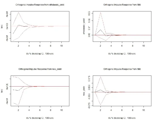
Figures 3 presents the orthogonalized impulse response function graphs of bitcoin’s and the cryptocurrencies’ return impulses and responses onto US equity market’s returns. Hence, testing the (H3a) “no cross-impact hypothesis a” in which these different asset classes should not have shocks onto each other.
20
Figures 3
These plots are to show the impulse of a variable and another variable’s response to it the system. In this case, it is the impulse from cryptocurrency’s daily yield and response to US equity market’s daily yield in percentage (decimal numbers) (y-axis) and vice versa. The x-axis shows the future estimation (lead effect) in days ranging from 10 to 20 days. The black line is daily yield (%) response to the said cryptocurrency or the equity and the dotted red lines display the statistical significance at α = 5 %. If the confidence interval (or band), bootstrap confidence level, does not contain zero (horizontal axis) then it is statistically significant.
22
From the plots can be deduced that cryptocurrencies and US equity market have no impulse response dynamics for estimation. This finding is in line with the (H3a) “no cross-impact hypothesis a” when addressing US equity market returns. Hence, based on US equity returns, the (H3a) hypothesis is not rejected at 5 % significance level.
5.2 OLS regressions
To further research the market relations (H3a&b) I construct various regressions while
controlling for Fama and French’s 3–factors (9), Carhart’s 4–factors (10) and using 5–factor model which includes the additional bitcoin momentum (11).
Table 2 presents regression where dependent variables (y) are bitcoin and the cryptocurrencies and explanatory variables are Fama and French’s 3–factors (9). Table 3 adds stock market momentum as an explanatory variable (10). Table 4 adds the bitcoin momentum to the 4–factor model (11).
23
Table 2
This table shows OLS regressions on cryptocurrencies (y) and their estimated coefficients explained in the methodology, in decimal numbers. On the same line with a coefficient name is the estimated decimal number values for it. Values inside parentheses are t-values. Significance codes (α): 0 ‘***’ 0.001 ‘**’ 0.01 ‘*’ 0.05 ‘.’.
Bitcoin Ethereum Dash Litecoin Ripple Monero NEM Ethereum
Classic NEO 𝛼 0.006*** 0.009** 0.010** 0.004* 0.005* 0.006** 0.012*** 0.015· 0.020** (4.445) (2.608) (3.160) (2.172) (2.401) (2.705) (3.766) (1.704) (2.704) 𝛽𝑅𝑚 0.067 0.102 0.040 -0.008 -0.066 -0.021 -0.661· -1.053 -0.019 (0.398) (0.265) (0.105) (-0.035) (-0.225) (-0.071) (-1.726) (-0.557) (-0.012) 𝛽𝑆𝑀𝐵 -0.060 -0.259 -1.230* -0.353 -0.177 0.114 -0.131 -0.840 -1.500 (-0.201) (-0.409) (-2.044) (-0.910) (-0.383) (0.245) (-0.209) (-0.434) (-0.914) 𝛽𝐻𝑀𝐿 -0.527· 0.438 0.318 0.053 -0.372 -0.254 0.519 -0.769 0.140 (-1.677) (0.752) (0.520) (0.131) (-0.772) (-0.542) (0.887) (-0.471) (0.100) Mult. R2 0.001 0.001 0.004 0.001 0.000 0.000 0.004 0.003 0.003 Adj. R2 -0.000 -0.003 0.002 -0.001 -0.001 -0.002 0.001 -0.004 -0.005
Using formula (9), the results suggest that cryptocurrencies have no market relations as expected. Alpha is positive and significant and R2 is low as they should. The (H3a) is not
rejected. The next Table 3 adds the market momentum factor as an additional explanatory variable.
24
Table 3
This table shows OLS regressions on cryptocurrencies (y) and their estimated coefficients explained in the methodology, in decimal numbers. On the same line with a coefficient name is the estimated decimal numbers values for it. Values inside parentheses are t-values. Significance codes (α): 0 ‘***’ 0.001 ‘**’ 0.01 ‘*’ 0.05 ‘.’.
Bitcoin Ethereum Dash Litecoin Ripple Monero NEM Ethereum
Classic NEO 𝛼 0.006*** 0.008** 0.010** 0.004* 0.005* 0.006** 0.012*** 0.014· 0.020** (4.446) (2.591) (3.128) (2.156) (2.399) (2.698) (3.761) (1.691) (2.710) 𝛽𝑅𝑚 0.066 0.059 0.002 -0.008 -0.066 -0.049 -0.703· -1.021 -0.112 (0.395) (0.152) (0.005) (-0.031) (-0.266) (-0.168) (-1.806) (-0.548) (-0.070) 𝛽𝑆𝑀𝐵 -0.068 -0.347 -1.355* -0.402 -0.180 0.034 -0.213 -0.861 -1.460 (-0.225) (-0.531) (-2.224) (-1.028) (-0.387) (0.072) (-0.331) (-0.441) (-0.884) 𝛽𝐻𝑀𝐿 -0.561 0.314 -0.036 -0.117 -0.383 -0.419 0.369 -0.792 0.191 (-1.639) (0.503) (-0.054) (-0.267) (-0.732) (-0.821) (0.581) (-0.479) (0.135) 𝛽𝑀𝑂𝑀 -0.059 -0.249 -0.577 -0.298 -0.019 -0.280 (-0.265) -0.152 0.395 (-0.253) (-0.565) (-1.298) (-1.034) (-0.055) (-0.816) (-0.607) (-0.089) (0.260) Mult. R2 0.001 0.002 0.005 0.001 0.000 0.001 0.005 0.003 0.003 Adj. R2 -0.000 -0.004 0.002 -0.001 -0.002 -0.002 0.000 -0.006 -0.007
The results are the almost identical with Table 3, which some weakening of alpha and improvement in R2. The (H3a) is not rejected. In the last Tables 4, 5 & 6 the bitcoin momentum
25
Table 4
This table shows OLS regressions on cryptocurrencies (y) and their estimated coefficients explained in the methodology, in decimal numbers. On the same line with a coefficient name is the estimated decimal number values for it. Values inside parentheses are t-values. Significance codes (α): 0 ‘***’ 0.001 ‘**’ 0.01 ‘*’ 0.05 ‘.’.
Bitcoin Ethereum Dash Litecoin Ripple Monero NEM Ethereum
Classic NEO 𝛼 0.006*** 0.009* 0.010** 0.003 0.004· 0.006* 0.012*** 0.016· 0.022** (3.862) (2.528) (3.168) (1.536) (1.927) (2.534) (3.701) (1.736) (2.702) 𝛽𝑅𝑚 0.054 0.063 0.012 -0.042 -0.105 -0.061 -0.694· -1.036 -0.120 (0.321) (0.160) (0.030) (-0.174) (-0.361) (-0.207) (-1.772) (-0.556) (-0.075) 𝛽𝑆𝑀𝐵 -0.069 -0.349 -1.345* -0.423 -0.215 0.027 -0.220 -0.911 -1.506 (-0.230) (-0.535) (-2.204) (-1.088) (-0.461) (0.056) (-0.342) (-0.466) (-0.910) 𝛽𝐻𝑀𝐿 -0.555 0.314 -0.034 -0.135 -0.415 -0.424 0.369 -0.775 0.213 (-1.624) (0.503) (-0.050) (-0.310) (-0.795) (-0.830) (0.581) (-0.468) (0.150) 𝛽𝑀𝑂𝑀 -0.061 -0.247 -0.562 -0.366 -0.080 -0.297 (-0.260) -0.046 0.482 (-0.262) (-0.560) (-1.260) (-1.274) (-0.234) (-0.862) (-0.594) (-0.027) (0.314) 𝛽𝛿 0.024** -0.004 -0.021 0.079*** 0.064** 0.028 -0.009 -0.043 -0.039 (2.685) (-0.089) (-0.530) (4.040) (2.633) (0.905) (-0.213) (-0.414) (-0.439) Mult. R2 0.004 0.002 0.005 0.011 0.005 0.002 0.005 0.003 0.003 Adj. R2 0.002 -0.005 0.001 0.008 0.002 -0.003 -0.001 -0.008 -0.010
The bitcoin momentum factor is significant when fitting bitcoin, litecoin, and ripple, which is the conclusion as in the orthogonalized impulse response function results. However, alphas diminish and lose their significance compared to Tables 2 and 3. Still, the (H3a) is not rejected. Results for testing (H3b) “no cross-impact hypothesis b”, are found in Table 5 and 6. Table 5 has value-weighted and equal-weighted regression coefficients for the full period and for subsamples for the banking industry (SIC code 45). Table 6 has the corresponding for the financial industry (SIC code 48).
26
Table 5
Value-weighted (VW) and equal-weighted (EW) regressions where dependent variable (y) is banking industry’s
excess returns and explanatory variables are as in Table 4.28 Full period constitutes the total 2599 trading days. Additionally, the data set is divided into 2 different periods (50/50) where the earlier period is the earlier data set timewise and the later period is the data set further away from today. On the same line with a coefficient name is the estimated decimal number values for it. Values inside parentheses are t-values. Significance codes (α): 0 ‘***’ 0.001 ‘**’ 0.01 ‘*’ 0.05 ‘.’. BANKS [45] VW full period EW full period VW earlier period EW earlier period VW later period EW later period 𝛼 -0.001 0.001*** 0.000 0.001*** -0.000 0.001*** (-1.435) (10.017) (0.011) (6.818) (-1.571) (8.774) 𝛽𝑅𝑚 1.186*** 0.601*** 1.200*** 0.664*** 1.162*** 0.569*** (112.591) (85.664) (73.972) (60.161) (87.070) (64.150) 𝛽𝑆𝑀𝐵 0.139*** 0.579*** 0.190*** 0.647*** 0.082** 0.538*** (7.293) (45.682) (7.322) (36.766) (3.085) (30.586) 𝛽𝐻𝑀𝐿 0.983*** 0.626*** 0.837*** 0.688*** 1.231*** 0.573*** (45.661) (43.663) (29.466) (35.609) (39.633) (27.743) 𝛽𝑀𝑂𝑀 0.051*** 0.088*** 0.128*** 0.167*** -0.070** -0.027· (3.537) (9.043) (6.766) (13.025) (-3.256) (-1.908) 𝛽𝛿 0.002*** 0.001 0.004* 0.002 0.002** 0.000 (3.396) (1.056) (2.528) (1.607) (2.864) (0.102) Mult. R2 0.880 0.880 0.837 0.834 0.923 0.903 Adj. R2 0.880 0.880 0.836 0.833 0.923 0.902
28 Detailed information about the classification of banking industry’s excess returns used is found in the Appendix B.
27
Firstly, the commonly accepted Carhart’s 4–factor coefficients are expectedly all significant across the table. Secondly, the interesting part is that in estimating banking industry’s value -weighted returns shows higher bitcoin momentum 𝛽𝛿 coefficient comparing to equal-weighted
returns. This implies that bitcoin momentum has a stronger effect on larger banks and institutions and weaker on smaller ones. Thirdly, the bitcoin momentum effect has grown over time and is stronger today than years ago.
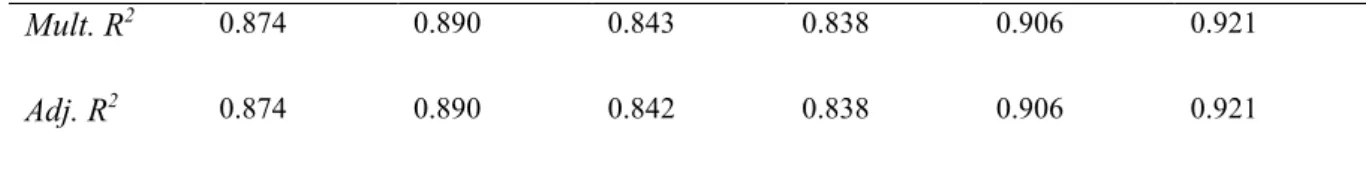
Table 6
Value-weighted (VW) and equal-weighted (EW) regressions where dependent variable (y) is financial industry’s
excess returns and explanatory variables are as in Table 4.29 Full period constitutes the total 2599 trading days. Additionally, the data set is divided into 2 different periods where the earlier period is the earlier data set timewise and the later period is the data set further away from today. On the same line with a coefficient name is the estimated decimal number values for it. Values inside parentheses are t-values. Significance codes (α): 0 ‘***’ 0.001 ‘**’ 0.01 ‘*’ 0.05 ‘.’. FIN [48] VW full period EW full period VW early period EW early period VW later period EW later period 𝛼 -0.000 -0.000 -0.000 -0.000 0.000 0.000 (-0.577) (-0.004) (-0.263) (-0.070) (0.158) (0.224) 𝛽𝑅𝑚 1.267*** 0.960*** 1.287*** 0.947*** 1.244*** 0.958*** (114.619) (110.803) (77.780) (69.753) (82.628) (81.790) 𝛽𝑆𝑀𝐵 0.152*** 0.634*** 0.174*** 0.608*** 0.148*** 0.660*** (7.618) (40.487) (6.588) (28.109) (4.962) (28.418) 𝛽𝐻𝑀𝐿 0.698*** 0.390*** 0.663*** 0.350*** 0.760*** 0.436*** (30.886) (21.973) (22.918) (14.735) (21.625) (16.003) 𝛽𝑀𝑂𝑀 -0.020 -0.037** 0.088*** -0.018 -0.209*** -0.084*** (-1.296) (-3.064) (4.586) (-1.112) (-8.625) (-4.480) 𝛽𝛿 0.001* 0.001 0.006*** 0.005*** 0.001 0.000 (2.145) (1.639) (3.846) (3.867) (0.584) (0.198)
29Detailed information about the classification of banking industry’s excess returns used is found in the Appendix B.
28
Table 6 continues on this page.
Mult. R2 0.874 0.890 0.843 0.838 0.906 0.921
Adj. R2 0.874 0.890 0.842 0.838 0.906 0.921
Firstly, the commonly accepted Carhart’s 4–factor coefficients are expectedly all significant across the table as in Table 5. Secondly, the interesting part is that in estimating financial
industry’s value-weighted returns shows lower bitcoin momentum 𝛽𝛿 coefficient comparing to
equal-weighted returns. This implies that bitcoin momentum has a stronger effect on smaller financial institutions and weaker on larger ones, and is the opposite as with the banks. Thirdly, the bitcoin momentum effect has weakened from the beginning, which again, is completely opposite than with the banking industry.
These results (Table 5 and 6) provide evidence that bitcoin, and possibly the cryptocurrency
market, influences banking and financial industries’ excess returns. Thus, (H3b) “no cross-impact hypothesis b”, is rejected on 5 % significance level.
6. Discussion and Further Analysis
In this section, I undergo the results for main hypotheses in a descriptive manner and provide my own analysis of the results.
6.1 The liquidity trap
As hypothesized, my results are aligned with Wang’s (2014) that bitcoin does not suffer from a liquidity trap. Even though in my opinion, bitcoin will eventually fall into liquidity trap due to its fundamentals discussed in Section 2, it seems to enjoy relatively good liquidity today. This might stem from the increasing number of traders in the bitcoin and cryptocurrency
market. However, in the future when the pace of bitcoin supply slows down, the Sweeneys’
analogy might become more realistic.
6.2 Internal impulse response dynamics of the cryptocurrencies
Notable about the orthogonalized impulse response function plots is the high autocorrelation
amongst the cryptocurrencies. Past day’s returns seem to estimate well future price development, especially 𝑡 + 1 returns. However, bitcoin impulse has only statistical
29
days where daily price data is available. Notable is that these two cryptocurrencies have the most days of data, after bitcoin, which might explain these results. Another reason is that litecoin and ripple, as older cryptocurrencies, are technologically more related to bitcoin30
compared to e.g. ethereum which represents new and more sophisticated blockchain technology. Nevertheless, this result provides evidence that traders can reduce their idiosyncratic volatility31 within the cryptocurrency market, something that has not been studied
with various cryptocurrencies to my knowledge. 6.3 Cryptocurrencies’ relation to the US equity market
As the results from orthogonalized impulse response functions suggest, bitcoin and the cryptocurrencies have no relations with the US equity market which is consistent with
Gangwal’s (2016) paper reporting that between 2012 and 2016 adding bitcoin to international
investors’ portfolio yields a higher Sharpe ratio. This result is robust even with regressions
utilizing Fama and French’s 3–factor model as well as adding to it Carhart’s momentum
component. When adding bitcoin momentum factor to the Carhart’s model, the results converge with the orthogonalized impulse response function’s, providing evidence that bitcoin
affects on litecoin’s and ripple’s returns but not on the other top 6 cryptocurrencies. 6.4 Cryptocurrencies’ relation to the financial industry
The most interesting result from this thesis is that the bitcoin momentum explains both banking
and financial industry’s returns, even when controlling with Carhart’s 4–factors. With banking industry, the value-weighted regression is statistically significant compared to equal-weighted implying that bitcoin momentum affects larger institutions more. In addition, this effect has grown stronger during the last years, as the subsample regression suggest. With financial industry, based on the regressions, the direction points the opposite. Bitcoin effect is stronger with smaller institutions but it has diminished over the years.
These findings raise questions. Intuitively, financial industry’s smaller players, such as security
and commodity brokers, would have been more quickly aboard in the cryptocurrency market but now are reducing risks from this high volatility market which would explain the change in the subsamples. On the other hand, larger banking institutions which have been strongly against
30 Website: http://www.businessinsider.com/bitcoin-price-etherum-and-other-cryptocurrencies-compare-2017-9?r=US&IR=T&IR=T, date 30.11.2017
31 Idiosyncratic risk is risk that can be diversified by allocating resources (e.g. money) to multiple assets if they have less than 1 of correlation.
30
bitcoin32 and the cryptocurrencies in general, have realized that the market has grown so big
that they must commit to it.33
7. Conclusion
In this thesis, I have analyzed if bitcoin suffers from illiquidity, bitcoin’s leading effect among
the top cryptocurrencies and cross-asset dynamics between cryptocurrencies and US equity market and financial sector. In my study, I use daily data of 9 cryptocurrencies, including bitcoin, and daily data of US equity market, banking and financial industry with both value-weighted and equal-value-weighted excess returns.
Firstly, I calculated Amihud illiquidity premium for bitcoin and constructed bitcoin momentum factor. Secondly, I computed ACF, PACF, CCF and VAR(p) models which I used for plotting
orthogonalized impulse response functions to view bitcoin’s illiquidity, bitcoin’s leading effect
among cryptocurrencies and cryptocurrencies shocks to US equity market, and vice versa. Thirdly, I regressed 3, 4 and 5–factor models (fifth factor as the bitcoin momentum) to add robustness to US equity market relation analysis. Finally, I regressed the 5–factor model on
banking and financial industries’ excess returns.
My findings on bitcoin’s liquidity are consistent with Wang’s (2014) paper where he argues
that bitcoin market is liquid and does not suffer from a liquidity trap. However, this paper is
inconsistent with Sweeneys’ analogy that decentralized currency systems are prone to failure. Also, my thesis is consistent with Smith (2016), Baur et al. (2015) that cryptocurrencies can be classified as currencies based on their characteristics and have weak relations with another asset classes. In this study, I use US equity market as a benchmark to show that cryptocurrencies, as an asset class belonging to currencies, have no impulse response dynamics with each other. In addition, this paper is aligned with Gangwal’s (2016) study where he reports
that between 2012 and 2016, adding bitcoin to international investor’s portfolio yield a higher
ratio. My thesis confirms this and adds more cryptocurrencies to this list.
Moreover, this paper provides interesting findings of bitcoin momentum factor’s effect, controlling with Carhart’s (1995) 4–factors, on banking and financial industry’s excess returns. The bitcoin momentum’s effect has grown over time as a statistically significant estimator for
32 Website: https://www.forbes.com/sites/panosmourdoukoutas/2017/09/14/why-big-banks-attacked-bitcoin/#6dd45fa06c53, date 1.5.2017.
31
big banks’ and institutions’ excess returns. On the other hand, the bitcoin momentum has an opposite impact on financial industry’s excess returns. Meaning that the bitcoin momentum has a stronger effect on smaller institutions and it has weakened during the last years. I leave this finding for further studies, as this thesis focuses more on the descriptive analysis of the cryptocurrency market relations within and outside.
The results of this study offer three practical implications. Firstly, it provides evidence that the bitcoin does not suffer from a liquidity trap and the market is liquid enough for investors and cryptocurrency users. Secondly, only two of the 8 other cryptocurrencies analyzed in this study
are under bitcoin’s lead effect, making it possible to reduce idiosyncratic risk within
cryptocurrency portfolio. Finally, as the cryptocurrency market and US equity excess returns do not have significant impulse response dynamics, the cryptocurrencies make an interesting asset diversification class for investors seeking for diversification benefits.
32
APPENDIX A: ACF, PACF & CCF of bitcoin and cryptocurrencies
The interpretation of the graphs is the following, the x-axis illustrates the lead or lag in days. The y-axis shows the function and its result. The heading elaborates in 1–2 what function and series is in question, in 3–10 the said cryptocurrency’s CCF between bitcoin, the numbers inside the bracket show with how many days of data it is calculated (end date 29.09.2017) and the dotted blue line are the significance level (5 %). These plots present the following: number 1 is the ACF of bitcoin, number 2 is the PACF of bitcoin and 3–10 are CCFs between bitcoin and the said cryptocurrency.33
APPENDIX B: Industry variable definitions
This Appendix presents the banking industry’s BANKS [45] and financial industry’s FIN [48] SIC codes and the sub-industry’s belonging to the accumulating classification in the United States of America.
BANKS [45] FIN [48]
6000-6000 Depository institutions 6200-6299 Security and commodity brokers 6010-6019 Federal reserve banks 6700-6700 Holding, other investment offices 6020-6020 Commercial banks 6710-6719 Holding offices
6021-6021 National commercial banks 6720-6722 Investment offices
6022-6022 State banks - Fed Res System 6723-6723 Management investment, closed-end 6023-6024 State banks - not Fed Res System 6724-6724 Unit investment trusts
6025-6025 National banks - Fed Res System 6725-6725 Face-amount certificate office 6026-6026 National banks - not Fed Res System 6726-6726 Unit inv trusts, closed-end 6027-6027 National banks, not FDIC 6730-6733 Trusts
6028-6029 Banks 6740-6779 Investment offices
6030-6036 Savings institutions 6790-6791 Miscellaneous investing 6040-6059 Banks (?) 6792-6792 Oil royalty traders 6060-6062 Credit unions 6793-6793 Commodity traders 6080-6082 Foreign banks 6794-6794 Patent owners & lessors 6090-6099 Functions related to deposit banking 6795-6795 Mineral royalty traders 6100-6100 Nondepository credit institutions 6798-6798 REIT
6110-6111 Federal credit agencies 6799-6799 Investors, NEC 6112-6113 FNM
6120-6129 S&Ls
6130-6139 Agricultural credit institutions 6140-6149 Personal credit institutions (Beneficial) 6150-6159 Business credit institutions
6160-6169 Mortgage bankers 6170-6179 Finance lessors 6190-6199 Financial services
34
References
Amihud, Y., 2002. Illiquidity and stock returns: cross-section and time-series effects, Journal of Financial Markets, 5, 1, 31–56.
Baur, D. G., Hong, K., and Lee, A. D., 2015. Bitcoin: Medium of Exchange or Speculative Asset?
Blitz, D., Huij, J., Lansdorp, S., and Verbeek, M., 2013. Short-term residual reversal, Journal of Financial Markets, 16, 3, 477–504.
Box, G. E. P., and Jenkins, G. M., 1976. Time Series Analysis; Forecasting and Control, 1st
Edition, Holden-day, San Francisco.
Carhart, M. M., 1995. Survivor bias and persistence in mutual fund performance, Unpublished Ph.D. dissertation, Graduate School of Business, University of Chicago, Chicago, Ill.
Fama, E. F., and French, K. R., 1993. Common risk factors in the returns on bonds and stocks, Journal of Financial Economics, 33, 3–53.
Gangwal, S., 2016. Analyzing the Effects of Adding Bitcoin to Portfolio, International Journal of Economics and Management Engineering, 10, 10.
Greer, R. J., 1997. What is an Asset Class, Anyway?, The Journal of Portfolio Management, 23, 2, 86–91.
Lintner, J., 1965. The valuation of risk assets and the selection of risky investments in stock portfolios and capital budgets, Review of Economics and Statistics, 47, 13–37.
Lütkepohl, H., 2005. New Introduction to Multiple Time Series Analysis. 1st Edition,
Springer-Verlag Berlin Heidelberg, Berlin.
Pfaff, B., 2008. Analysis of Integrated and Cointegrated Time Series with R. 2nd Edition.
Springer, New York. ISBN 0-387-27960-1.
Sharpe, W. F., 1964. Capital Asset Prices: A theory of market equilibrium under conditions of risk, Journal of Finance 19, 425–42.
Shaub, D. 2014. Testing the Efficient Market Hypothesis on Bitcoin Exchanges, Master’s thesis
dissertation, Department of Economics, Uppsala University, Uppsala.
Smith, J. 2016. An Analysis of Bitcoin Exchange Rates, University of Houston, Houston. Sweeney, J., and Sweeney, R. J., 1977. Monetary Theory and the Great Capitol Hill Baby Sitting Co-op Crisis: Comment, Journal of Money, Credit and Banking, 9, 1, 86–89.
Usoro, A. E., 2015. Some basic properties of cross-correlation functions of n-dimensional vector time series. Journal of Statistical and Econometric Methods, 4, 1, 63–71.
Venables, W. N., and Ripley, B. D., 2002. Modern Applied Statistics with S. Fourth Edition. Springer-Verlag.
Wang, J., C-Y., 2014. A Simple Macroeconomic Model of Bitcoin, Working paper, Bitquant Research Laboratories.