Sequentially-fit alternating least squares algorithms in nonnegative matrix factorization

(1)

c

(2)

SEQUENTIALLY-FIT ALTERNATING LEAST SQUARES

ALGORITHMS

IN NONNEGATIVE MATRIX FACTORIZATION

BY

FLORIAN MARKUS LORENZ

THESIS

Submitted in partial fulfillment of the requirements

for the degree of Master of Arts in Psychology

in the Graduate College of the

University of Illinois at Urbana-Champaign, 2010

Urbana, Illinois

Master’s Committee:

Professor Lawrence Hubert, Chair

Assistant Professor Sungjin Hong

(3)

Abstract

Nonnegative matrix factorization (NMF) and nonnegative least squares regres-sion (NNLS regresregres-sion) are widely used in the physical sciences; this thesis explores the often-overlooked origins of NMF in the psychometrics literature. Another method originating in psychometrics is sequentially-fit factor analy-sis (SEFIT). SEFIT was used to provide faster solutions to NMF, using both alternating least squares (ALS) with zero-substitution of negative values and NNLS. In a simulation using SEFIT for NMF, differences in fit between the ALS-based solution and the NNLS-based solution were minimal; both solutions were substantially faster than standard whole matrix based approaches to NMF.

(4)

(5)

Acknowledgments

First, I would like to thank my parents, Judith and Dieter Lorenz, without whose moral and financial support college - never mind graduate school - would not have been feasible. My thanks also go to Han Hui Por for constant moral support during these difficult times and, hopefully, all good and bad times in the future. I also owe gratitude to Dr. Stephen Broomell, who made graduate school more bearable through humor.

I would like to thank Professor Lawrence Hubert, my thesis adviser, who helped me become interested in this topic and was my patient guide on this rocky path. Thanks also go to Professor Sungjin Hong, the second reader of this thesis, especially for his excellent feedback.

I would also like to thank the psychology department for supporting me as a teaching assistant for many quantitative psychology courses, and at the time of this writing, greatly increasing the amount of available time for thesis research by assigning me the teaching assistant position for a cognitive psychology course. Furthermore, I wish to express my gratitude to the Herbert Woodrow Founda-tion, whose fellowship has allowed me time to work on research.

(6)

List of Tables

3.1 Means and Standard Deviations of Variance-Accounted-For, Pro-portion of Runs that produce the best VAF, and Time in All Conditions for NMF-SZ. . . 10 3.2 Means and Standard Deviations of Variance-Accounted-For,

Pro-portion of Runs that produce the best VAF, and Time in All Conditions for NMF-FNNLS. . . 11 3.3 Means and Standard Deviations of Variance-Accounted-For,

Pro-portion of Runs that produce the best VAF, and Time in All Conditions for NMF-SEFIT. . . 11 3.4 Means and Standard Deviations of Variance-Accounted-For,

Pro-portion of Runs that produce the best VAF, and Time in All Conditions for NMF-NNLS-SEFIT. . . 12

(8)

List of Figures

3.1 Relation Between Quality of Solution (as Measured by Variance-Accounted-For) and Error Level for All Four Algorithms. . . 12 3.2 Relation Between Error Level and Computation Time for All

Four Algorithms. . . 13 3.3 Relation Between Error Level and Computation Time for All

(9)

Chapter 1

History of Nonnegative

Matrix Factorization

Many articles about nonnegative matrix factorization (NMF) neglect to give an accurate account of the origins of the method. Those papers that do de-scribe its development seem to imply that in the early 1990s NMF sprang from the computational biology / chemistry / physics field, like Athena from Zeus’ forehead. In fact, NMF builds on a long tradition of factor analytic methods that originated in psychometrics over eight decades before the terminology of “Nonnegative Matrix Factorization“ was even coined.

1.1

Model

Nonnegative matrix factorization (NMF) is a constrained version of factor anal-ysis (FA), perhaps the most important method developed in psychometrics. FA was developed by the eminent psychologist Charles Spearman during his inves-tigation of intelligence during the first decade of the 20th _{century [19]. This} research led to the theory of generalized intelligence, which is the basis of many modern methods of aptitude assessment, such as IQ testing. FA also underlies many current models in personality and social psychology and is widely used in the physical and social sciences, and applied areas such as marketing.

The factor analytic model usually decomposes a m×m correlation or co-variance matrix for m variables, but can also be used to decompose a n×m

matrixY of measurements fromnsubjects onmvariables into an×k matrix

Fofnfactor scores onkfactors, anm×kmatrixAof factor loadings and an

n×mresidual matrixE:

Y=FAT +E. (1.1)

This can also be represented as a sum of outer products:

Y= k

X

j=1

fjaj, (1.2)

wherefj is thejthcolumn of Fandaj is thejthcolumn of A.

It is immediately apparent that this model does not have a unique solution because any unitary matrix R (that is, any matrix for which the conjugate transpose of R is equal to the inverse of R) can be inserted into the above

(10)

equation: Y=FRRTAT+E=F ˙˙AT +E, where ˙ F=FR, ˙ AT =RTAT

This lack of a unique solution is termed rotational indeterminacy; the psy-chometrics literature provides a large number of rotation methods that produce ideal factorizations satisfying different criteria.

The basic factor analytic model can be defined stochastically by assuming distributions for the data and, as a consequence, the component matrices F

and A and residual matrices or by imposing orthogonality constraints on the columns of the product matrices. The FA model has also been expanded to allow the analysis of N-way (rather than two-way) data, including Tucker models, Par-allel Factor Analysis (Parafac) and Individual Differences Scaling (INDSCAL) models; a thorough review of all extensions of FA is well beyond the scope of this work and can be found elsewhere.

Nonnegative matrix factorization (NMF) is essentially a constrained FA model. NMF methods take ann×mdata matrixXand factor it into a num-ber of product matrices and an n×m residual matrix E. The elements of at least one of the product matrices and usually the data matrix is constrained to be within the space of positive numbersR+, that is, nonnegative. The most

widely recognized of these models approximately factors the data matrix into two nonnegative product matrices,W(n×k)and H(m×k),

X=WHT+E, X∈R+, (1.3)

where each entry inW,wij ≥0 and each entry inH,hij ≥0 for alli, j. Like FA, NMF is subject to rotational indeterminacy.

The basic NMF model has been modified in various ways. Some NMF models require only one of two product matrices to consist of nonnegative entries, others impose additional constraints such as column-wise orthogonality (e.g., [7]) or sparsity (e.g., [8]) on the product matrices. The two-way NMF model has been expanded to analyze N-way data in the form of constrained Tucker models (e.g., [9] )and constrained PARAFAC [14].

In addition to factoring a data matrix into substantively interpretable prod-uct matrices, both FA and NMF can be used to reduce the dimensionality of the data, that is, the rank of the product matrixFAT, or WHT, respectively. This goal is accomplished by reducing the number of columns of the first com-ponent matrix and the number of rows of the second comcom-ponent matrix to some number k <rank(Y) for FA or k < rank(X) for NMF. Smaller values of k al-low more parsimonious interpretations of the data whereas larger values of k

(11)

1.2

Sequentially Fitted Clustering as NMF

Clustering refers to the sorting of a set of data into categories. These categories either can be non-overlapping (in “hard“ or “discrete“ clustering) or overlapping (in “fuzzy“ or “probabilistic“ clustering). There exists a number of different ap-proaches to clustering, including hierarchical clustering, eigenvector-based clus-tering (spectral clusclus-tering), and clusclus-tering methods based on partitions, such as

k-means clustering.

Ink-means clustering, first proposed by Lloyd [16], the number of clusters to be formed is determined a priori. Initial centroids (cluster centers) are chosen either randomly or by means of a heuristic. Data points are then assigned to clusters corresponding to the respectively closest centroids; once all data points have been assigned, centroids are updated based on the members of their clus-ters and data points re-sorted into the clusclus-ters with the closest (now updated) centroid. This process iterates until centroids no longer change. The procedure, as might be expected, is prone to local optima.

Variants of this method differ in the frequency of centroid updates (e.g. after removing and reassigning a single data point rather than all data points) and in the manner in which centroids are calculated – by modes (k-modes), by medians (k-medians) and by weighted means.

The relationship between clustering and FA representation is well known. Dis-crete cluster analysis can be written as

X=WAT+E, (1.4)

whereAis unconstrained and contains centroid vectors for each of thekclusters and the entries in the n×k matrix W determine cluster membership. W

therefore has entries of only 1 (for membership in a cluster) and 0, with the additional constraint that there is only a single entry of 1 in each row (i.e. that each object belongs in only one cluster). [17].

Probabilistic cluster analysis can be related to FA by means of the same equation, with different constraints: the columns of W are nonnegative and sum to 1, that is, members of a constrained subset of non-negative values; furthermore, the sum of any column must be greater than zero [17].

It is not hard to see that equation (1.4) can be written as a sum of vector products in the manner of equation (1.2):

X= k

X

j=1

wjaj (1.5)

The implication is that the clustering structure can be fit sequentially: first

Xis approximated by an outer product, this outer product is then subtracted fromXto form a residual matrix. This residual matrix is then approximated by another vector product, and so on, untilkvector products have been found: The

(12)

Program 1Sequential fitting procedure forX≈WAT

for j = 1 ... k

find wj, aj that minimize (X−wjaj)

X=X−wjaj

end

component vectors in (1.5) can be found be Eckart-Young decomposition ofX; another way is by alternation least squares, similarly to the method described for FA, above.

WhenXis a distance matrix, its entries are nonnegative and this approach to clustering becomes an NMF model where only one product matrix is constrained to be nonnegative; this is sometimes termed ”semi-NMF” [5]. It is also of interest that the alternating least-squares (ALS) sequential fitting method proposed by Mirkin in the cited 1990 article iteratively estimates the columns of W and

A, setting negative entries to zero; this is the essence of the most widely used method of solving the NMF problem, re-discovered in 1994.

1.3

Individual Differences Scaling as NMF

Individual Differences Scaling (INDSCAL) models between-subjects differences in the perceived distances of a set of stimuli and has been used extensively in a number of different fields. INDSCAL has a number of parallels with Parafac; both are used for three-way data. In fact, the original article presented IND-SCAL alongside Canonical Decomposition (Candecomp), which is essentially identical to Parafac [4], and was used to fit the INDSCAL model; Parafac and Candecomp are considered to be independently developed.

The nonnegativity of the INDSCAL model is a the result of of the symmetry of the model:

Xj=QDjQ T ₊_E

j,

whereXj is then×nslice of the three-way arrayXcorresponding to subject

j,Q is a collection of stimulus-dimension vectors andDj is a diagonal matrix of subject-specific weights for the vectors inQ. The original article [4] specified that these weights should be nonnegative, making this the first published NMF model (though, admittedly, not the most general). The algorithm used for this factorization (Candecomp) usually produced nonnegative weights but could not guarantee it; in practice, negative values were ignored. A solution to INDSCAL that assures the nonnegativity of D by using NNLS in the weight estimation was found in 1993 [20].

(13)

1.4

NMF Re-invented by Paatero and

Popularized by Lee and Seung

The first widely-cited article describing the special case of NMF in which the data matrix and both product matrices are constrained toR+ was published as

“Positive Matrix Factorization“ in 1994 by Paatero [18] and described a specially constrained alternating least squares algorithm. A second article by the same author [15] provided a similar algorithm with a number of application-specific modifications. It is likely due to the decidedly non-straightforward manner in which the algorithms were coded and the relative obscurity of the journals in which they were published that neither article received much attention; they are still not as widely cited as other similar articles. There is some irony in this as the papers in question do not cite any works on the development of FA - the basis for NMF - other than a comment that FA “originates in the soft sciences”. The first popular article on NMF methodology was published inNaturein 1999 and presented a clear description of a multiplicative update NMF algorithm [13]; again, this latter piece failed to cite any sources from the substantial body of factor analytic-methodology developed in psychometrics.

(14)

Chapter 2

Computational methods for

solving NMF

2.1

Multiplicative Update Based Methods

Because the algorithms given in one of the most widely cited papers on NMF [13] multiplicative update strategies enjoy great popularity. An interesting feature of multiplicative update algorithms is that once an entry in an estimated product matrix becomes zero, it tends to remain zero across iterations; well-initialized starting matrices are therefore especially important for this class of algorithms. Although this property hints at the tendency of multiplicative update algorithms to converge to local optima, it can also be advantageous when the product matrices are to be sparse.

A further property of all multiplicative update algorithms is the relatively slow convergence relative to other types of algorithms, especially those that are least squares based.

A large number of multiplicative update algorithms exist and can differ sub-stantially based on the cost function used. Since the focus of this paper is on additive update least squares algorithms for NMF, this section aims only to provide an introduction to multiplicative update methods for the sake of completeness. A through review can be found elsewhere, e.g., in [6].

Among the first multiplicative update algorithms to receive widespread at-tention, the Lee and Seung algorithms [13] rely on minimizing the squared Eu-clidean distance between the data matrixAand the product matricesWHby iteratively updatingWandH.

Program 2Lee and Seung Multiplicative Update NMF Algorithm set criterionvalue

W ∈R+n×k, H ∈R + m×k

while criterion<criterionvalue Wnew = W .∗( (AW)T ./ (WHHT + ) )

Hnew = H .∗( (WnewA) ./ (WTnewWnewA + ) ) compute criterion

H = Hnew W = Wnew end

(15)

Here, ”.∗” represents the Hadamard (i.e., element-by-element) product and ”./” is the element-by-element division of two matrices.

A variety of stopping criteria can be considered. First, the algorithm might be stopped after a certain number of iterations. Although this has the disadvan-tage of not ensuring numerical convergence, it does prevent an infinite loop. A second stopping criterion might be the difference between the original data ma-trix and the estimated data mama-trix computed from the product matrices. This difference is often measured in terms of sums of squared differences, but might feasibly be based on some other measure, such as the determinant of the differ-ence matrix. One disadvantage of this approach is that it is difficult to estimate a priori what this difference should be given that NMF is only an approximate factorization. A third criterion might be based on iteration-to-iteration changes of the entries in the product matrices. If these entries cease to change, at least a local optimum must have been reached. At a global optimum, the solution indicated by a lack of change in parameters is identical to that indicated by the sum of squares difference measure if the model is unique. In practice, a combination of these three stopping criteria is generally used.

2.2

Alternating Least Squares Algorithms for

NMF

Given that one method of performing a FA is by means of alternating least squares (ALS) algorithms, applying this method to NMF seems natural. There are two possible strategies to constrain the results to be nonnegative. One approach computes a least-squares solution and then eliminates any negative values; the other uses an ALS algorithm designed to produce only nonnegative results.

2.2.1

Zero-Substitution ALS

The simplest way to eliminate negative entries in a matrix is to set them to zero. Zero-substitution ALS solutions to NMF add only a small step to FA ALS algorithms. First, one of the product matrices is initialized, either with random values or some starting estimate. Then, the least squares estimate of the second product matrix given the first product matrix is computed. Any negative entries of the estimated second product matrix are set to zero. Based on the estimated second product matrix, the first product matrix is re-computed; any negative entries in this estimated matrix are set to zero. At this point, the algorithm either returns to the first estimation step or terminates if some criterion has been met.

(16)

Program 3Alternating Least Squares NMF Algorithm set criterionvalue

W ∈R+n×k, H ∈R + m×k

while criterion6=criterionvalue Hnew = (WTW)−1WTA

set all wi < 0 to 0 Wnew = (HnewHTnew)−1HnewAT Set all hi < 0 to 0 compute criterion H = Hnew

W = Wnew end

As with multiplicative update algorithms, a number of measures, each with its own advantages and disadvantages can be used as stopping criteria.

2.2.2

Nonnegative Least Squares Based Algorithms

A framework for solving nonnegativity constrained regression problems has ex-isted for close to three decades and has seen extensive use in chemometrics, where NMF is also widely used. Although the original active-set-based nonneg-ative least squares (NNLS) algorithm by Lawson and Hanson [12] was designed to solve equation systems of they=Xbtype, it can easily be adapted for use in NMF. The speed of an unmodified implementation of Lawson-Hanson NNLS (LH-NNLS) leaves something to be desired, however [10].

Fast NNLS (fNNLS), a first step in improving NNLS, capitalizes on the iter-ative nature and nonnegativity constraints in NNLS [3]. An even faster version of fNNLS relies on combinatorial arguments to decrease the computational bur-den of NNLS by re-arranging the order in which calculations are performed [1]. When used for NMF, fast combinatorial NNLS (fcNNLS) results in an algorithm that marginally outperforms fNNLS-based approaches to the same problem [10]. Because the convergence properties of NNLS are well-documented, it is widely held that LH-NNLS, fNNLS and fcNNLS-based NMF algorithms are also guar-anteed to converge. This certainty comes at price, however: these algorithms are far slower than zero-substitution-based ALS algorithms.

(17)

Chapter 3

Experimental Comparison

of ALS Methods

There is little research on SEFIT-based NMF algorithms. The only paper on this topic [5] fails to outline the development of NMF as a constrained FA method and presents “Hierarchical NMF” as a completely new method rather than an application of SEFIT to NMF. Furthermore, only the feasibility of SEFIT-based NMF and a vague outline of how it might be implemented are discussed. The results of the simulation run in this article are given only as histograms, without any interpretable comparisons of either inter-algorithm differences in computa-tion time or solucomputa-tion quality.

3.1

Algorithms

Four algorithms were compared (1) a zero-substitution ALS NMF algorithm SZ), (2) a sequentially-fit zero-substitution ALS NMF algorithm (NMF-SEFIT), (3) a NNLS based NMF algorithm (NMF-NNLS), and (4) a sequentially-fit NNLS based NMF algorithm (NMF-NNLS-SEFIT).

The NMF-SZ algorithm consisted of the algorithm included in the Matlab Bioin-formatics toolbox, NNMF.m. The NMF-NNLS algorithm was based on an ex-isting algorithm by Kim and Park. [8] and used a Matlab implementation of the fcNNLS algorithm by Bro et al. [3]. The NMF-SEFIT and NMF-NNLS-SEFIT algorithms were designed to be very similar, except that NMF-SEFIT relies on zero-substitution during the alternating estimation of each vector product, while NMF-NNLS-SEFIT calls fcNNLS. The codes for NMF-SEFIT, NMF-NNLS and NMF-NNLS-SEFIT is are included as appendices.

3.2

Data

The aim of this study was to compare the four algorithms both in terms time required to compute a solution and in terms of quality of that solution, measured as variance-accounted-for (VAF). In addition to examining solutions with four, five and six latent factors, five different error levels (5, 10, 20, 30, and 40 percent) were examined; this yielded 15 conditions.

An important challenge in the development of NMF methods today is the large size of the data sets usually analyzed. Thus, 20 matrices of size 5000×50

(18)

were created as follows for each condition: First, two matrices of uniform random numbers ranging from zero to twenty, W5,000×k and H50×k, were generated.

The product of these matrices,WHT_{, was added to a matrix}_E_{of uniform} ran-dom error ranging from−to +, wheredepended on the specified error level. Any entries in the resulting matrixX=WHT₊_E_{that were not in}

R+were set to

zero. Each of the four algorithms was run 20 times, until either convergence was achieved or 10,000 iterations were reached. The variance-accounted-for (VAF) and the time required for an algorithm to terminate for each run were saved.

3.3

Results

The means and standard deviations of both VAF and time and the proportion of runs that produced the best solution (as indicated by the highest VAF) over all runs within a condition by algorithm are reported in Tables 3.1, 3.2, 3.3 and 3.4.

Factors Error Mean(VAF) SD(VAF) p(VAFbest) Mean(time) SD(time)

4 0.05 0.94 0.00259 0.16 2.386 0.03767 0.10 0.80 0.00177 0.13 2.387 0.02549 0.20 0.53 0.00142 0.13 2.397 0.02063 0.30 0.33 0.00081 0.10 2.393 0.02324 0.40 0.24 0.00049 0.10 2.389 0.02408 5 0.05 0.93 0.00239 0.09 2.935 0.02686 0.10 0.79 0.00254 0.07 2.946 0.02310 0.20 0.50 0.00175 0.06 2.933 0.02942 0.30 0.33 0.00089 0.07 2.934 0.02482 0.40 0.24 0.00057 0.08 2.937 0.03910 6 0.05 0.93 0.00441 0.07 3.278 0.02488 0.10 0.78 0.00317 0.06 3.281 0.03058 0.20 0.49 0.00204 0.06 3.278 0.02997 0.30 0.33 0.00099 0.06 3.283 0.02754 0.40 0.25 0.00061 0.07 3.283 0.02641

Table 3.1: Means and Standard Deviations of Variance-Accounted-For, Pro-portion of Runs that produce the best VAF, and Time in All Conditions for NMF-SZ.

(19)

Factors Error Mean(VAF) SD(VAF) p(VAFbest) Mean(time) SD(time) 4 0.05 0.94 0.00001 0.99 31.842 1.61488 0.10 0.80 0.00000 1.00 13.414 0.71205 0.20 0.53 0.00001 0.99 8.860 0.71856 0.30 0.34 0.00002 0.89 12.698 2.40750 0.40 0.24 0.00000 0.97 11.747 2.17791 5 0.05 0.93 0.00001 0.99 44.060 1.73606 0.10 0.79 0.00004 0.93 22.136 2.94918 0.20 0.51 0.00007 0.90 14.025 2.49676 0.30 0.33 0.00004 0.82 19.748 4.68052 0.40 0.25 0.00003 0.88 20.372 6.09388 6 0.05 0.93 0.00002 0.98 44.495 2.16550 0.10 0.78 0.00003 0.94 23.921 3.46006 0.20 0.49 0.00007 0.86 21.504 7.08591 0.30 0.33 0.00004 0.84 26.988 8.54497 0.40 0.25 0.00005 0.85 29.204 9.42756

Table 3.2: Means and Standard Deviations of Variance-Accounted-For, Pro-portion of Runs that produce the best VAF, and Time in All Conditions for NMF-FNNLS.

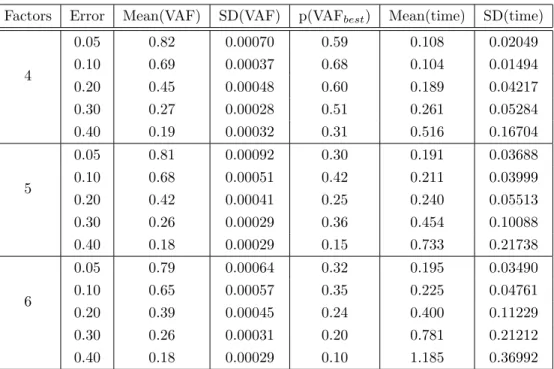
Factors Error Mean(VAF) SD(VAF) p(VAFbest) Mean(time) SD(time)

4 0.05 0.82 0.00070 0.59 0.108 0.02049 0.10 0.69 0.00037 0.68 0.104 0.01494 0.20 0.45 0.00048 0.60 0.189 0.04217 0.30 0.27 0.00028 0.51 0.261 0.05284 0.40 0.19 0.00032 0.31 0.516 0.16704 5 0.05 0.81 0.00092 0.30 0.191 0.03688 0.10 0.68 0.00051 0.42 0.211 0.03999 0.20 0.42 0.00041 0.25 0.240 0.05513 0.30 0.26 0.00029 0.36 0.454 0.10088 0.40 0.18 0.00029 0.15 0.733 0.21738 6 0.05 0.79 0.00064 0.32 0.195 0.03490 0.10 0.65 0.00057 0.35 0.225 0.04761 0.20 0.39 0.00045 0.24 0.400 0.11229 0.30 0.26 0.00031 0.20 0.781 0.21212 0.40 0.18 0.00029 0.10 1.185 0.36992

Table 3.3: Means and Standard Deviations of Variance-Accounted-For, Pro-portion of Runs that produce the best VAF, and Time in All Conditions for NMF-SEFIT.

(20)

Factors Error Mean(VAF) SD(VAF) p(VAFbest) Mean(time) SD(time) 4 0.05 0.82 0.00111 0.59 0.757 0.10722 0.10 0.69 0.00036 0.68 0.801 0.11447 0.20 0.45 0.00047 0.57 1.281 0.26395 0.30 0.27 0.00028 0.53 2.043 0.41998 0.40 0.19 0.00030 0.37 4.350 1.46847 5 0.05 0.81 0.00079 0.36 1.113 0.20732 0.10 0.68 0.00061 0.43 1.210 0.18568 0.20 0.42 0.00044 0.28 1.995 0.46304 0.30 0.26 0.00026 0.39 4.083 0.89226 0.40 0.18 0.00029 0.13 6.780 1.90857 6 0.05 0.79 0.00071 0.29 1.603 0.30350 0.10 0.65 0.00058 0.31 1.824 0.33937 0.20 0.39 0.00042 0.26 3.478 0.90775 0.30 0.26 0.00031 0.22 6.846 2.03741 0.40 0.18 0.00029 0.14 11.193 3.70307

Table 3.4: Means and Standard Deviations of Variance-Accounted-For, Pro-portion of Runs that produce the best VAF, and Time in All Conditions for NMF-NNLS-SEFIT.

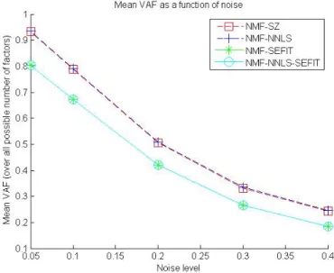
Unsurprisingly, the mean VAF was inversely related to error level, regardless of the number of latent factors in the data or the algorithm used (see Figure 3.1).

Figure 3.1: Relation Between Quality of Solution (as Measured by Variance-Accounted-For) and Error Level for All Four Algorithms.

(21)

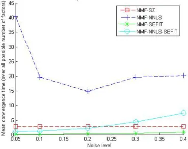
a function of noise level, convergence time did not follow any apparent overall pattern (see Figure 3.2). The convergence time of NMF-SZ was relatively invari-ant over error levels. For both NMF-SEFIT and NMF-NNLS-SEFIT, the error increased in a curvilinear fashion; the rate of increase was far greater for the latter algorithm (see Figure 3.3). Convergence time decreased for NMF-FNNLS until an error level of 20 percent; after this, it increased (see Figure 3.2).

Figure 3.2: Relation Between Error Level and Computation Time for All Four Algorithms.

Figure 3.3: Relation Between Error Level and Computation Time for All NMF-SZ, NMF-SEFIT and NMF-NNLS-SEFIT.

(22)

As expected, NMF-NNLS was both the slowest and the most accurate al-gorithm; for any given error level and number of latent factors, it produced the highest mean VAF and the highest mean time. Furthermore, NMF-NNLS proved to be more consistent than the other algorithms: it had the lowest VAF standard deviation in any condition and produced the best solution on between 82 percent and 100 percent of the random restarts, depending on condition.

NMF-SZ consistently produced mean VAFs within 0.01 units of those pro-duced by NMF-NNLS; it was also much faster, on average taking only 12.5 percent of the time required by NMF-NNLS. Regardless of condition, NMF-SZ also higher VAF standard deviations than NMF-NNLS; the average VAF stan-dard deviation was about 60 times higher than that of NMF-FNNLS. This may indicate that NMF-SZ is more likely to converge to a local, rather than global optimum than NMF-NNLS. The propensity for this algorithm to get stuck at local optima is further illustrated by the low proportion of runs during which the best solution was produced: this topped out at 16 percent for the lowest error level and number of factors and consistently decreased as the number of factors and errors increased, to a minimum of 6 percent. NMF-SZ was also less consistent than NMF-SEFIT and NMF-NNLS-SEFIT; the mean VAF for NMF-SZ was about 3.8 times greater than those two algorithms.

NMF-SEFIT proved to be the fastest algorithm; on average, it converged in about 0.17 percent of the time required by NMF-FNNLS, in about 11.7 percent of the time required by NMF-NNLS-SEFIT and 13.4 percent of the time required by NMF-SZ. Additionally, NMF-SEFIT was more consistent than NMF-SZ: the best solution was found on between 68 and 10 percent of all runs, depending on condition.

This speed came at a price, however; on average, the mean VAF produced by NMF-SEFIT was 0.092 units lower than that produced by NMF-SZ. This difference was highly dependent on the overall level of error in the data: at 5 percent error, average VAF difference was about 0.13, whereas at 40 percent error, the average VAF difference was about 0.06 (Figure 2).

Using NNLS estimation in sequential fitting proved not to be profitable: although it was faster than either NMF-SZ or NMF-NNLS, NMF-NNLS-SEFIT was slower than NMF-SEFIT in all conditions and produced virtually identical mean VAFs with slightly higher standard deviations.

3.4

Discussion

Of the numerous least squares based methods for solving the NMF, methods using NNLS estimation are widely believed to be the most accurate and among the slowest; the current study confirmed this finding. The reputation of zero-substitution based ALS methods for NMF to be nearly as accurate as NNLS based methods but far faster was also confirmed.

(23)

equa-tion is part of most descripequa-tions of FA. A through investigaequa-tion of the quality and speed of sequentially-fit NMF solutions had not been attempted prior to this study. We found that when a rank-reduced solution was desired, NNLS based sequentially fit NMF is considerably faster than even zero-substitution based NMF; zero-substitution based NMF-SEFIT is faster yet. Both methods of sequentially-fit NMF produced factorizations of virtually identical quality; the fits were somewhat worse than those of the two whole-matrix based NMF methods. This difference in solution quality decreased substantially with in-creasing error. Given the reduction in fit, NFM-SEFIT may not be the most useful method when the matrix to be factored is relatively small as the time savings are not substantial in this case. For example, a 5000×50 matrix can be factorized in less than a minute on a reasonably fast personal computer by the slowest algorithm used in this study. In larger-scale problems or real-time ap-plications, especially those with relatively noisy data, SEFIT based NMF could prove valuable, however. Given the drastic decrease in computation time that SEFIT-based methods displayed when performing an NMF, it may be worth-while to investigate the use of SEFIT-based methods for N-way data analysis methods, e.g. nonnegatively constrained PARAFAC models.

(24)

References

[1] van Benthem, M.,&Keena, M. (2005). Fast algorithm for the solution of large-scale non-negativity-constrained least squares problems. Journal of Chemometrics, 18, 441 – 450.

[2] van Benthem, M. et. al. REFERENCE MISSING.

[3] Bro, R., & De Jong, S. (1997). A fast non-negatively constrained least squares qlgorithm.Journal of Chemometrics, 11, 393 – 401.

[4] Carroll, J.,&Chang, J. (1970). Analysis of individual differences in mul-tidimensional scaling via an N-way generalization of “Eckart - Young” decomposition.Psychometrika, 35, 267 – 283.

[5] Cichocki, A., Zdunek, R., & Amari, S. (2007). Hierarchical ALS algo-rithms for nonnegative matrix and 3D tensor factorization.Lecture Notes in Computer Science, 169 – 176.

[6] Cichocki, A., Zdunek, R., Phan, A., & Amari, S. (2009). Nonnegative matrix and tensor factorizations. Applications to exploratory multi-way data analysis and blind source separation. Chinchester, England: Wily. [7] Ding, C., Li, T., Peng, W., & Park, H.(2006). Orthogonal nonnegative

matrix trifactorizations for clustering. Proceedings of the ACM SIGKDD International Conference on Knowledge Discovery and Data Mining, pp 126 – 135, Philadelphia, PA, USA

[8] Kim, H.,&Park, H. (2007). Sparse non-negative matrix factorizations via alternating non-negativity-constrained least squares for microarray data analysis.Bioinformatics, 23, 1495 – 1502.

[9] Kim, Y.,&Choi, S. (2007). Nonnegative Tucker decomposition. Proceed-ings of the IEEE CVPR-2007 Workshop on Component Analysis Methods, Minneapolis, Minnesota, USA.

[10] Kim, H., & Park, H. (2008). Nonnegative matrix factorization based on alternating nonnegativity constrained least squares and active set method.

SIAM Journal of Matrix Analysis and Applications, 30, 713 – 730. [11] Kolda, T., &Bader, B. (2009). Tensor decompositions and applications.

SIAM Review, 51, 455 – 500.

[12] Lawson, C., &Hanson, R. (1981). Solving least squares problems. Engle-wood Cliffs, NJ: Prentice-Hall.

[13] Lee, D.,&Seung, D. (1999). Learning the parts of objects by non-negative matrix factorization.Nature, 401, 788 – 791.

(25)

[14] Lim, L. (2005). Optimal solutions to nonnegative PARAFAC / multilinear NMF always exist.Workshop of Tensor Decompositions and Applications. CIRM, Luminy, Marseille, France.

[15] Leea, E., Chan, C., & Paatero, P. (1999). Application of positive matrix factorization in source apportionment of particulate pollutants in Hong Kong.Atmospheric Environment, 33, 3201 – 3212.

[16] Lloyd, S. P. (1957). Least square quantization in PCM. Bell Telephone Laboratories Paper.

[17] Mirkin, B. (1990). A sequential fitting procedure for linear data analysis models.Journal of Classification, 7, 167 – 195.

[18] Paatero, P., & Tapper, U. (1994). Positive matrix factorization: A non-neagtive factor model with optimal utilization of error estimates of data values.Environmetrics, 5, 111 – 126.

[19] Spearman, C. (1904). General intelligence objectively determined and measured.American Journal of Psychology, 15, 201 - 293.

[20] Ten Berge, J., Kiers H.,&Krijnen, W. (1993). Computational solutions for the problem of negative saliences and nonsymmetry in INDSCAL.Journal of Classification, 10, 115 – 124.

(26)

Appendix A

Code for NMF-SEFIT

function [W H] = nmf_sefit(X,K)

%%NMF_SEFIT performs a sequentially fitted (SEFIT) nonnegative matrix %%factorization (NMF).

%Factor analysis can be performed by SEFTI (Mikrin, 1990). Here, the method %is extended to NMF: X = WH’, where x_ij, h_ij, h_ij all E R^+

% %Input:

%X an (n by p) data matrix, with x_ij E R^+

%k an integer from 1 to rank(X), giving the rank of the solution %

%Output:

%W the first (n by k) product matrix, with w_ij E R^+ %H the second (p by k) product matrix, with h_ij E R^+ %

%Florian Lorenz January 11, 2010

%set values for stopping criterion critval = 10^-10;

%save data matrix for later use, get data matrix dimensions initX=X;

[n,m]=size(X);

%initialize product matrices, empty for W, random numbers for H W=zeros(n,K);

H=rand([m,K]);

%set variables needed to stop ALS loop to dummy values criterion = 1;

oldW = W; oldH = H;

%sequential fitting loop for k=1:K

(27)

%precompute X’ Xt=X’;

%iteration count to prevent getting stuck iter=1;

%alternating least squares (ALS) loop while criterion > critval;

%compute vector for W based on vector in H W(:,k) = ( X * H(:,k)) / sum( ( H(:,k) ).^2 ); %set elements that are R^- to zero

W(:,k) = max(0,W(:,k));

%compute vector for H based on vector in W

H(:,k) = ( Xt * W(:,k) ) / sum ( ( W(:,k) ).^2 ); %set elements that are R^- to zero

H(:,k) = max(0,H(:,k));

%compute value for stopping criterion wdiff = max(max(abs(W(:,k)-oldW(:,k)))); hdiff = max(max(abs(H(:,k)-oldH(:,k)))); criterion = max(wdiff,hdiff);

oldW = W; oldH = H;

%break out of loop if stuck iter=iter+1;

if iter > 10000 break; end

end

%updata data matrix X=X-W(:,k)*H(:,k)’; %re-set criterion criterion = 1; end

(28)

Appendix B

Code for NMF-NNLS

function [W H] = nmf_fnnls(X,K)

%%NMF_FNNLS performs a sequentially fitted nonnegative matrix factorization %%(NMF) using fast combinatorial nonnegative least squares estimateion %%(fcNNLS).

%This code is based on nnmfsh_comb.m, a sparsity-coinstrained, fcNNLS-based %NMF algorithm by Kim and Park (2007). Like nnmfsh_comb.m, nmf_fnnls uses %fcnnls.m, a fast combinatorial nonnegative least squares estimation %algorithm by Van Benthem and Keenan (2004).

% %Input:

%Output:

[n,m]=size(X);

H=rand([m,K]);

%set variables needed to stop ALS loop to dummy values oldW = W;

(29)

criterion = 1;

%alternating nonnegative least squares (ANLS) loop while criterion > critval;

%disp(iter); %estimate W based on H Wt=fcnnls(H,X’); W=Wt’; %estimate H based on W Ht = fcnnls(W,X); H=Ht’;

%compute value for stopping criterion wdiff = max(max(abs(W-oldW)));

hdiff = max(max(abs(H-oldH))); criterion = max(wdiff,hdiff); oldW = W;

oldH = H;

(30)

Appendix C

Code for NMF-NNLS-SEFIT

function [W H] = nmf_sefit_nnls(X,K)

%%NMF_SEFIT_NNLS performs a sequentially fitted (SEFIT) nonnegative matrix %%factorization (NMF) using fast combinatorial nonnegative least squares %%estimateion (fcNNLS).

%Factor analysis can be performed by SEFTI (Mikrin, 1990). Here, the method %is extended to NMF: X = WH’, where x_ij, h_ij, h_ij all E R^+

%This algorithm uses fcnnls.m, a fast combinatorial nonnegative least %squares estimation algorithm by Van Benthem and Keenan (2004). %

%Input:

%Output:

[n,m]=size(X);

H=rand([m,K]);

%set variables needed to stop ALS loop to dummy values criterion = 1;

oldW = W; oldH = H;

(31)

%sequential fitting loop for k=1:K

%precompute X’ Xt=X’;

%alternating least squares (ALS) loop while criterion > critval;

%compute vector for W based on vector in H %W(:,k) = ( X * H(:,k)) / sum( ( H(:,k) ).^2 ); W(:,k) = fcnnls(H(:,k),X’)’;

%set elements that are R^- to zero %W(:,k) = max(0,W(:,k));

%compute vector for H based on vector in W

%H(:,k) = ( Xt * W(:,k) ) / sum ( ( W(:,k) ).^2 ); H(:,k) = fcnnls(W(:,k),X)’;

%set elements that are R^- to zero %H(:,k) = max(0,H(:,k));

%compute value for stopping criterion wdiff = max(max(abs(W(:,k)-oldW(:,k)))); hdiff = max(max(abs(H(:,k)-oldH(:,k)))); criterion = max(wdiff,hdiff);

oldW = W; oldH = H;

end

%updata data matrix X=X-W(:,k)*H(:,k)’; %re-set criterion criterion = 1; end

Sequentially-fit alternating least squares algorithms in nonnegative matrix factorization