A Programming Language for Data Privacy with Accuracy Estimations

(1)

Thesis for the Degree of Licentiate of Philosophy

A Programming Language for Data

Privacy with Accuracy Estimations

Elisabet Lobo Vesga

Department of Computer Science and Engineering Chalmers University of Technology

(2)

Technical Report 214L ISSN 1652-876X

Department of Computer Science and Engineering Research group: Information Security

Department of Computer Science and Engineering Chalmers University of Technology

SE-412 96 Göteborg Sweden

Telephone +46 (0)31-772 1000 Printed at Chalmers

(3)

Abstract

Differential privacy offers a formal framework for reasoning about privacy and accuracy of computations on private data. It also offers a rich set of building blocks for constructing private data analyses. When carefully calibrated, these analyses simultaneously guarantee the pri-vacy of the individuals contributing their data, and the accuracy of the data analyses results, inferring useful properties about the population. The compositional nature of differential privacy has motivated the de-sign and implementation of several programming languages aimed at helping a data analyst in programming differentially private analyses. However, most of the programming languages for differential privacy proposed so far provide support for reasoning about privacy but not for reasoning about the accuracy of data analyses. To overcome this limi-tation, in this work we present DPella, a programming framework pro-viding data analysts with support for reasoning about privacy, accuracy and their trade-offs. The distinguishing feature of DPella is a novel com-ponent which statically tracks the accuracy of different data analyses. In order to make tighter accuracy estimations, this component leverages taint analysis for automatically inferringstatistical independenceof the different noise quantities added for guaranteeing privacy. We evaluate our approach by implementing several classical queries from the litera-ture and showing how data analysts can figure out the best manner to calibrate privacy to meet the accuracy requirements.

Keywords:accuracy, concentration bounds, differential privacy, func-tional programming, databases, haskell

(4)

(5)

Acknowledgments

First, I would like to express my sincere appreciation to Alejandro Russo, my supervisor, for his patient guidance, inspiring enthusiasm, and constant encouragement. I would also like to thank my co-supervisor and collaborator, Marco Gaboardi, for his detailed lessons on probability and invaluable mentorship.

My thanks are extended to my friends and colleagues for their fel-lowship, the easy laughs, and insightful conversations. It is an honor to share this experience with all of you.

I wish to acknowledge the support, prayers, and great love of my family who set me off on this journey a long time ago. Last but not least, a special recognition goes to my partner Alejandro Gómez for being my rock from the very beginning. I will always be grateful to have you by my side.

(6)

(7)

Introduction

Motivation

Differential privacy (DP) [17] is emerging as a viable solution to release statistical information about the population without compromising data subjects’ privacy. A standard way to achieve DP is adding some statistical noise to the result of a data analysis. If the noise is carefully calibrated, it provides aprivacyprotection for the individuals contributing their data, and at the same time it enables the inference ofaccurateinformation about the population from which the data are drawn. Thanks to its quantitative formulation quantifying privacy by means of the parameters

andδ, DP provides a mathematical framework for rigorously reasoning

about theprivacy-accuracy trade-offs. The accuracy requirement is not baked in the definition of DP, rather it is a constraint that is made explicit for a specific task at hand when a differentially private data analysis is designed.

An important property of DP iscomposeability: multiple differen-tially private data analyses can be composed with a graceful degradation of the privacy parametersandδ. This property allows to reason about

privacy as abudget: a data analyst can decide how much privacy budget (theparameter) to assign to each of her analyses. The

compositional-ity aspects of DP motivated the design of several programming frame-works [38, 49, 48, 25, 21, 4, 5, 61, 58, 31, 60, 62] and tools [36, 42, 39, 23] with built-in basic data analyses to help analysts to design their own dif-ferentially private consults. At a high level, most of these programming frameworks and tools are based on a similar idea for reasoning about privacy: use some primitives for basic tasks in DP as building blocks, and use composition properties to combine these building blocks mak-ing sure that the privacy cost of each data analysis sum up and that the total cost does not exceed the privacy budget. Programming frameworks such as [38, 49, 48, 25, 21, 4, 5, 61, 58, 31, 60, 62] also provide general sup-port to further combine, through programming techniques, the different building blocks and the results of the different data analyses. Differently,

(10)

of restricting the kinds of data analyses they can support.

Unfortunately, this simple approach for privacy cannot be directly applied to accuracy. Reasoning about accuracy isless compositionalthan reasoning about privacy, and it depends both on the specific task at hand and on the specific accuracy measure that one is interested in offering to data analysts. Despite this, when restricted to specific mechanisms and specific forms of data analyses, one can measure accuracy through estimates given asconfidence intervals, or error bounds. As an example, most of the standard mechanisms from the differential privacy literature come with theoretical confidence intervals or error bounds that can be exposed to data analysts in order to allow them to take informed decisions about the consults they want to run. This approach has been integrated in tools such as GUPT [42], PSI [23], and Apex [24]. Users of these tools, can specify the target confidence interval they want to achieve, and the tools adjust accordingly the privacy parameters, when sufficient budget is available1_.

In contrast, all the programming frameworks proposed so far [38, 49, 48, 25, 21, 4, 5, 61, 58, 31, 60, 62] do not offer any support to programmers or data analysts for tracking, and reasoning about, the accuracy of their data analyses. This phenomenon is in large part due to the complex nature of accuracy reasoning, with respect to privacy analyses, when designing arbitrary data analyses that users of these frameworks may want to program and run. In this work, we address this limitation by building a programming framework for designing differentially private analysis which also supports a compositional form of reasoning about accuracy.

Background

We start by providing a brief background on the notions of privacy and accuracy DPella considers. Differential privacy [17] is a quantitative notion of privacy that bounds how much a single individual’s private data can affect the result of a data analysis. More formally, we can

1_{Apex actually goes beyond this by also helping user by selecting the right} differen-tially private mechanism to achieve the required accuracy.

(11)

define differential privacy as a property of a randomized query _Q˜₍_·₎ representing the data analysis, as follow.

Definition 1. Differential Privacy (DP)[17] A randomized query ˜

Q(·) : db→_Rsatisfies-differential privacyif and only if for any two datasetsD1andD2 indb, which differ in one row, and for every output setS⊆_Rwe have

Pr[ ˜Q(D1)∈S]6ePr[ ˜Q(D2)∈S] (1)

In the definition above, the parameterdetermines a bound on the

distance between the distributions induced by_Q˜₍_·₎ _{when adding or} removing an individual from the dataset—the farther away they are, the more at risk the privacy of an individual is, and vice versa. In other words,imposes a limit on theprivacy lossthat an individual can incur in, as a result of running a data analysis.

A standard way to achieve -differential privacy is adding some

carefully calibrated noise to the result of a query. To protect all the different ways in which an individual’s data can affect the result of a query, the noise needs to be calibrated to the maximal change that the result of the query can have when changing an individual’s data. This is formalized through the notion ofsensitivity.

Definition 2. [17]The(global) sensitivityof a queryQ(·) : db→Ris the quantity∆Q = max{|Q(D1)−Q(D2)|forD1, D2 differing in one row

The sensitivity gives a measure of the amount of noise needed to protect one individual’s data. Besides, in order to achieve differential privacy, it is also important the choice of the kind of noise that one adds. A standard approach is based on the addition of noise sampled from the Laplace distribution.

Theorem 1. Laplace Mechanism [17] LetQ(·) : db → _Rbe a de-terministic query with sensitivity∆Q. LetQ˜(·) : db→Rbe a random-ized query defined asQ˜(D) = Q(D) +η, whereηis sample from the Laplace distribution with meanµ = 0and scaleb =∆Q/. ThenQ˜ is

-differentially private.

Notice that in the theorem above, for a given query, the smaller the

(12)

how meaningful the result of the query is—and vice versa. In general, the notion ofaccuracycan be defined more formally as follows.

Definition 3. Accuracy, see e.g.[15] Given an-differentiallly private queryQ˜(·), a target queryQ(·), a distance functiond(·), a boundα, and the probabilityβ, we say thatQ˜(·)is(d(·), α, β)-accuratewith respect to

Q(·)if and only if for all datasetD:

Pr[d( ˜Q(D)−Q(D))> α]6β (2)

This definition allows one to express data independent error state-ments such as: with probability at least1−βthe queryQ˜(D)diverge fromQ(D), in terms of the distanced(·), for less thanα. Then, we will

refer toαas theerrorand1−βas theconfidence probability or simply confidence. In general, the lower theβis, i.e., the higher the confidence

probability is, the higher the errorαis.

As previously discussed, an important property of differential privacy is composeability.

Theorem 2. Sequential Composition [17] LetQ˜1(·)andQ˜2(·)be two

queries which are1- and2-differentially private, respectively. Then, their sequential compositionQ˜(·) = ( ˜Q1(·),Q2˜ (·))is(1+2)-differentially private.

Theorem 3. Parallel Composition [38] LetQ˜(·)be a-differentially private query. anddata1,data2 be a partition of the set of data. Then,

the queryQ˜1(D) = ( ˜Q(D∩data1),Q˜(D∩data2))is-differentially

private. Thanks to the composition properties of differential privacy, we can think aboutas aprivacy budget that one can spend on a given data before compromising the privacy of individuals’ contributions to that data. Theglobalfor a given program can be seen as the privacy budget

for the entire data. This budget can be consumed by selecting thelocalto

“spend” in each intermediate query. Thanks to the composition properties, by tracking the localthat are consumed, one can guarantee that a data

analysis will not consume more than the allocated privacy budget. Given an, DPella gives data analysts the possibility to explore how

to spend it on different queries and analyze the impact on accuracy. For instance, data analysts might decide to spend “more” epsilon on sub-queries which results are required to be more accurate, while spending

(13)

“less” on the others. The next examples (inspired by the use of DP in network trace analyses [37]) show how DPella helps to quantify what “more” and “less” means.

Contribution

The main contribution of this thesis is showing how programming frame-works can internalize the use ofprobabilistic bounds[14] for compos-ing different confidence intervals or error bounds, in an automated way. Probabilistic bounds are part of the classical toolbox for the analysis of randomized algorithms, and are the tools that differential privacy algo-rithms designers usually employ for the accuracy analysis of classical mechanisms [15, 18]. Two important probabilistic bounds are theunion bound, that can be used to compose errors with no assumption on the way the random noise is generated, andChernoff bound, which applies to the sum of random noise when the different random variables characterizing noise generation are statistically independent (see Section 3). When appli-cable, and when the number of random variables grows, Chernoff bound usually gives a much “tighter” error estimation than the union bound.

Barthe et. al [8] have shown how the union bound can be internal-ized in a Hoare-style logic for reasoning about probabilistic imperative programs, and how this logic can be used to reason in a mechanized way about the accuracy of probabilistic programs, and in particular of programs implementing differentially private primitives.

Building on this idea, this thesis proposes a programming framework where this kind of reasoning is automated, and can be combined with reasoning about privacy. The aim of such framework is to offer program-mers the tools that they need for implementing differentially private data analyses and explore their privacy-accuracy trade-offs, in a composi-tional way. This framework supports not only the use of union bound as a reasoning principle, but also the use of the Chernoff bound. The insight is that probabilistic bounds relying on probabilistic independence of ran-dom variables can be smoothly integrated in a programming framework by using techniques from information-flow control [52] (in the form of taint analysis [53]). While these probabilistic bounds are not enough to express every accuracy guarantee one wants to express for arbitrary data analyses, they allow the analysis of a large class of user-designed pro-grams. The approach to be presented in this thesis allows programmers to exploit the compositional nature of both privacy and utility,

(14)

comple-PSI [23], which yield confidence intervals estimate only at the level of in-dividual queries, and by Apex [24], which issue confidence intervals esti-mate only at the level of a query workload for queries of the same type. The described tool is materialized as a programming framework called DPella —an acronym for Differential Privacy in Haskell with accuracy— where data analysts can explore the privacy-accuracy trade-off while writing their differentially private data analyses. DPella pro-vides several basic differentially private building blocks and composition techniques, which can be used by a programmer to design complex dif-ferentially private data analyses. The analyses that can be expressed in DPella aredata independentand can be built using primitives for count-ing, average, max as well as any aggregation of their results.

DPella supports both pure-DP, with parameter, and

approximate-DP, with parametersandδ. Accordingly, it supports the use of both

Laplace and Gaussian noise, and the use of sequential or advanced [15] composition, respectively, together with parallel composition for both notions. For clarity, this thesis will mainly focus on-DP and will present

the use of the Laplace mechanism, however other variants will be dis-cussed briefly (see Section 3.3). DPella is implemented as a library in the general purpose language Haskell; a programming language that is well-known to easily support information-flow analyses [34, 50]. Further-more, DPella is designed to beextensiblethrough the addition of new primitives (see Section 6).

To reason about privacy and accuracy, DPella provides two primi-tives responsible to symbolically interpret programs (which implement data analyses). DPella’s symbolic interpretation for privacy consists on decreasing the privacy budget of a query by deducing the required bud-get of its sub-parts. On the other hand, the accuracy interpretation uses as abstraction theinverse Cumulative Distribution Function(iCDF) rep-resenting an upper bound on the (theoretical) error that the program incurs when guaranteeing DP. The iCDF of a query is build out of the iCDFs of the different components, by using as a basic composition prin-ciple theunion bound. These interpretations provide overestimates of the corresponding quantities that they track. In order to make these esti-mates as precise as possible, DPella usestaint analysisto track the use of noise to identify which variables arestatistically independent. This in-formation is used by DPella tosoundlyreplace, when needed, the union bound with theChernoff bound, something that to the best of our

(15)

knowl-edge other program logics or program analyses also focusing on racy, such as [8] and [54], do not consider. We envision DPella’s accu-racy estimations to be used in scenarios which align with those consid-ered by tools like GUPT, PSI, and Apex.

In summary, this thesis contributions are:

I Present DPella, a programming framework that allows data analysts

to reason compositionaly about privacy-accuracy trade-off.

I Show how to use taint analysis to detect statistical independence of

the noise that different primitives add, and how to use this information to achieve better error estimates.

I Inspect DPella’s expressiveness and error estimations by

implement-ing PINQ-like queries from previous work [37, 38, 3] and workloads from the matrix mechanism [33, 28, 59].

Thesis structure

This thesis is an extended version of the work “A Programming Frame-work for Differential Privacy with Accuracy Concentration Bounds” to be published inThe 41st IEEE Symposium on Security and Privacy (S&P 2020), San Francisco, USA, May 2020. The referred paper was created in collaboration with Alejandro Russo and Marco Gaboardi.

This document is structured as follows. Section 1 introduces DPella by showcasing its main features though simple examples. Section 2 presents each of DPella’s primitives for the construction and execution of queries. Section 3 explains how do we calculate accuracy concentration bounds and the accuracy-aware primitives that can be used by the data analysts. On Section 4 we implement case studies from the literature revealing DPella’s advantages and limitations. Section 5 introduces a new primitive that allows data analysts to test DPella’s accuracy estimations. Following, on Section 6 we discuss DPella’s limitations in detail together with possible extensions to the framework. Lastly, Section 7 puts DPella in context while contrasting it with other approaches and frameworks. This work was initiated by a STINT Initiation grant (IB 2017-77023) and supported by the Swedish Foundation for Strategic Research (SSF) under the project Octopi (Ref. RIT17-0023) and WebSec (Ref. RIT17-0011) as well as the Swedish research agency Vetenskapsrådet.

(16)

(17)

1

DPella by example

DPella’s model considers two kind of actors:data curators, owners of the private dataset that decide the global privacy budget and split it among thedata analysts, the ones who write queries to mine useful information from the data and spend the budget they received. Analysts are not allowed to directly query the database, instead, they need to implement their analyses and send them to the curator which will execute them and give the results back.

project SchemaDB.hs analysts Queries.hs curator Execution.hs dataset.csv

Figure 1:File structure

From an implementation standpoint, it means that the analyses and their run func-tions are provided in different files, with dif-ferent privileges. More specifically, Figure 1 depicts a common file structure for the us-age of DPella. FileSchemaDB.hscontains

the schema of the database own by the cu-rator, it does not contain private data, only the names of the tables and their respective attributes as a Haskell record type. For ex-ample, a database containing just one table calledAgeswith two attributesname(aStringvalue) andage(anInt

value), will be encoded inSchemaDB.hsas follows, where(::)is used to describe the type of a term in Haskell:

dataAges=AgeRow{name::String,age::Int}

Since the structure of the database is not considered sensitive informa-tion,SchemaDB.hscan be accessed by both, the data owners and data

analysts.

FileQueries.hscontains the analyses that have being implemented

by the data analysts, all of these queries should be parameterized by the dataset in which they will be later executed. Analysts will only

(18)

have access to their implementations and the database schema. Lastly, fileExecution.hs implements the run functions for the analyses at Queries.hs, this file is own by the curator and has access to all other

files in the directory, in particular, it has access to the real data—stored indataset.csv.

1.1 Basic aggregations

For the following examples, we consider a dataset representing atcpdump trace of packets where each row contains the information indicated by its schema:

dataTcpdump=TCPRow{id ::Integer

,timestamp::Double ,src ::IP ,dest ::IP ,protocol ::Integer ,size ::Integer ,payload ::ByteString } 1.1.1 Counting

An analyst wanting to know the number of packets sent toWikiLeaks, with IP address195.35.109.53, can do so by writing a simpleeps

-differentially private query as follows: importSchemaDB

importAnalystLP

−

wikileaks::→Data1Tcpdump→Query(ValueDouble)

wikileaks eps dataset=do

byIP←dpWhere((≡195.35.109.53)◦dest)dataset

dpCounteps byIP

First, we import file SchemaDB where Tcpdump’s description

(previ-ously presented) is stored. Then, we import DPella’s interface for ana-lysts calledAnalystLP, whereLPindicates that we will use the

(19)

1.1. Basic aggregations

takes as input the amount of privacy budgeteps(of type) to be spent

by the query and the dataset (of type Data 1 Tcpdump) where it

will be computed; when executed, this query will yield results of type

Query(ValueDouble), that is, DPella computations of typeDouble—a

more detailed explanation of DPella’s types could be found in the follow-ing sections. In querywikileaks, we use the primitive transformation2

dpWhereto filter all rows whose destattribute has a value equal to

195.35.109.53, this operation returns a transformed dataset that we have calledbyIP. We proceed to perform the noisy count using

primi-tivedpCountover the filtered datasetbyIPwhile spendingepsamount

of privacy budget. The value ofepswill—internally—determine the

mag-nitude of noise to be added to the real count.

Having this general implementation, an analyst can write specific queries fixing the value ofeps, for instance:

analysis1=wikileaks0.5

analysis2=wikileaks1

analysis3=wikileaks5

To execute these analyses the data owner needs to implement a function that loads the required dataset and execute analysts’ queries, such a function will look like:

importSchemaDB

importCuratorLP(loadDS,dpEval) importQueries

−

runAnalysis :: (Data1Tcpdump→Query(ValueDouble))

→→IO Double runAnalysis query bud=do

ds←loadDS"hotspot.csv" dpEvalquery ds bud

FunctionrunAnalysistakes as inputs the function to be executed, called query, and the global privacy budgetbud; returning the randomized

count as anIO Double. This function calls an auxiliar functionloadDS

(provided by DPella’s interface for curators) to read filehotspot.csv

2_{Anticipating on Section 2, in our code we will usually use the red color for} trans-formations, the blue color for aggregate operations, and the green color for combinators for privacy and accuracy.

(20)

which is then saved as a DPella’s dataset in variableds. Next, it uses

DPella’s primitivedpEvalindicating which analysis will be perform, over which dataset, and what’s the tolerance for the privacy loss.

Let’s assumehotspot.csvhave the information of10,000packets and7of them where directed to wikileaks’ IP address. Then, when the data owner executes the analysis she would get results such as:

>runAnalisis analysis120 Value=15.3 >runAnalisis analysis220 Value=4.8 >runAnalisis analysis320 Value=6.7

Which clearly exemplifies the effects of the selection of eps on the

queries’ results. Intuitively, the greater theeps, the closer we are to the

real count of packets.

1.1.2 Sums

Suppose we are now interested in computing the amount of transmit-ted data. This is, we want to sum up the value ofsizecolumn which

indicates the length of the packets in bytes.

In DPella, to compute a sum, we need to determine first the range of the values—our framework supports only natural numbers’ ranges, e.g., [1,10],[5,10], etc. This information is needed to automatically calculate

the sensitivity of sum queries at compile time, i.e., if every value is in the range[a, b], the sensitivity isb−a. The way to specify ranges in DPella

is via the primitive range.

range:: (Nata,Natb,Nat(b-a),a6b)⇒Range a b

This function receives no arguments since the range is indicated at the type-level (with type constraints of the formNatn). To create

ranges, we need to use type applications, e.g.,

range1=range @1 @10

range2=range @5 @10

For our specific case, the data curator indicates that the range of the size of packets go from40to35,000bytes, then we define our query as follows:

(21)

1.2. Cumulative Distribution Function

totalBytes eps dataset=do

dpSumeps(range @40 @35000)size dataset

FunctiontotalBytesuses primitivedpSumto compute the noisy sum

ofsizeattribute—whose values are ranging from40to35000bytes— over the indicateddataset. The way this query should be executed

does not vary from the execution of the analyses derived from function

wikileaks, thus is omitted.

Changing the question to focus on an specific protocol might require an adjustment on the range to be specified. For instance, if instead we want to inspect the total amount of data transmitted through Kerberos’ authentication protocol, which uses port 88, we should use the fact that this port transmits packets of at most of1465bytes. Hence, we will need to update our query accordingly

totalBytesKerberos eps dataset=do

kerberos←dpWhere((≡88)◦protocol)dataset

dpSumeps(range @40 @1465)size kerberos

In functiontotalBytesKerberoswe will first filter the dataset to obtain

the information regarding port 88, then we perform the noisy sum over the filtered data. Observe that we are defining a query with less global sensitivity than the one implemented in functiontotalBytes, thus, if

given the sameeps, less noise will be added to the results of the analyses

deriving from functiontotalBytesKerberos.

Having a notion of the order of magnitude in which the result of a sum ranges becomes handy when reasoning about the accuracy of the query.

In the following examples we depict how an analyst can use DPella to inspect the error of her queries, check out for miscalculations on the consumption of the privacy budget, and more.

1.2 Cumulative Distribution Function

Considering the same datasetTcpdumpwe would like to inspect—in a

differentially private manner—the packet’s length distribution by com-puting its Cumulative Distribution function (CDF), defined as CDF(x) = number of records with value6x. Hence, we are just interested in the

(22)

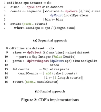
1 cdf1 bins eps dataset=do

2 sizes ←dpSelectsize dataset

3 counts←sequence [doelems←dpWhere(6bin)sizes

4 dpCountlocalEps elems

5 |bin←bins]

6 return(norm∞counts)

7 wherelocalEps=eps/(length bins)

(a)Sequential approach

8 cdf2 bins eps dataset=do

9 sizes←dpSelect((6max bins)◦size)dataset

10 --parts::Map Integer(ValueDouble)

11 parts←dpPartRepeat(dpCounteps)bins assignBin

12 sizes

13 letcounts =Map.elems parts

14 cumulCounts= [ add(take i counts) 15 |i←[1.length counts]] 16 return(norm∞cumulCounts)

(b)Parallel approach

Figure 2:CDF’s implementations

McSherry and Mahajan [37] proposed three different ways to ap-proximate (due to the injected noise) CDFs with DP, and they argued for their different levels of accuracy. For simplicity, we revise two of these approximations to show how DPella can assist in showing the accuracy of these analyses.

1.2.1 SequentialCDF

A simple approach to compute the CDF consists in splitting the range of lengths intobinsand, for eachbin, count the number of records

that are6bin. A natural way to make this computation differentially

private is to add independent Laplace noise to each count.

We show how to do this using DPella in Figure 2a. We define a function cdf1 which takes as input the list of binsdescribing size

ranges, the amount of budgetepsto be spent by the entire query, and

thedatasetwhere it will be computed. For now, we assume that we

have a fixed list of bins for packets’ length.cdf1uses the primitive

(23)

packet via a selector function, in this case it is just the column of interest

size. This computation results in a new datasetsizes. Then, we create

a counting query for each bin using the primitivedpWhere. This filters all records that are less than thebinunder consideration (6bin). Finally,

we perform a noisy count using primitivedpCount. The noise injected

by the primitivedpCountis calibrated so that the execution ofdpCount

islocalEps-DP (line 73). The functionsequencethen takes the list of

queries and compute them sequentially collecting their results in a list— to create a list of noisy counts. We then return this list. The combinator norm∞in line 6 is used to mark where we want the accuracy information

to be collected, but it does not have any impact on the actual result of the cdf.

To ensure thatcdf1iseps-differential privacy, we distributed the

given budgetepsevenly among the sub-queries (this is done in lines 4

and 7). However, a data analyst may forget to do so, e.g., she can define

localEps=eps, and in this case the final query is(length bins)*eps

-DP, which is a significant change in the query’s privacy price. To pre-vent such budget miscalculations or unintended expenditure of privacy budget, DPella provides the analyst with the functionbudget(see

Sec-tion 2) that, given a query, statically computes an upper bound on how much budget it will spend. To see how to use this function, consider the functioncdf1and a its modified versioncdf1’withlocalEps=eps.

Suppose that we want to compute how much budget will be consumed by running it on a list of bins of size 10 (identified asbins10) and a

sym-bolic datasetsymDataset. Then, the data analyst can ask this as follows:

>budget(cdf1bins101symDataset) =1

>budget(cdf1’bins101symDataset) =10

The functionbudgetwill notexecute the query, it simply performs an static analysis on the code of the query by symbolically interpreting it. The static analysis uses information encoded by thetypeofsymDataset

(explained in Section 2), that, in this particular case, will be provided by

Tcpdump’s schema.

DPella also provides primitives to statically explore the accuracy of a query. The functionaccuracytakes a noisy queryQ˜(·)and a probability

(24)

βand returns an estimate of the (theoretical) error that can be achieved

with confidence probability1−β. Suppose that we want to estimate the

error we will incur in by runningcdf1with a budget of= 1with the same list of bins and symbolic dataset as above, and we want to have this estimate forβ = 0.05andβ= 0.2, respectively. Then, the data analyst can ask this as follow:

>accuracy(cdf1bins101symDataset)0.05 α=53

Since the result of the query is a vector of counts, we measure the errorαin terms of`∞distance with respect to the CDF without noise. This is the max difference that we can have in a bin due to the noise. The way to read the information provided by DPella is that with confidence 95%and80%, we have errors53and40, respectively. These error bounds can be used by a data analyst to figure out the exact set of parameters that would be useful for her task.

1.2.2 ParallelCDF

Another way to compute a CDF is by first generating an histogram of the data according to the bins, and then building a cumulative sum for each bin. To make this function private, an approach could be to add noise at the different bins of the histogram, rather than to the cumulative sums themselves, so that we could use the parallel composition, rather than the sequential one [37], which we show how to implement in DPella in Figure 2b. —where double-dashes are used to introduce single-line comments.

Incdf2, we first select all the packages whose length is smaller than

the maximum bin, and then we partition the data accordingly to the given list of bins. To do this, we usedpPartRepeatoperator to create as many (disjoint) datasets as givenbins, where each record in each partition

be-longs to the range determined by an specificbin—where the record

be-longs is determined by the functionassignBin::Integer→Integer.

After creating all partitions, the primitivedpPartRepeatcomputes the given querydpCountepsineach partition—the namedpPartRepeat comes from repetitively callingdpCount epsas many times as

(25)

the keys are thebinsand the elements are the noisy count of the records

per partition—i.e., the histogram. In what follows (lines 14–16), we com-pute the cumulative sums of the noisy counts using the DPella primitive add, and finally we build and return the list of values denoting the CDF.

The privacy analysis ofcdf2is similar to the one ofcdf1. The

ac-curacy analysis, however, is more interesting: first it gets error bounds for each cumulative sum, then these are used to give an error bound on the maximum error of the vector. For the error bounds on the cumula-tive sums DPella uses either the union bound or the Chernoff bound, depending on which one gives the lowest error. For the maximum error of the vector, DPella uses the union bound, similarly to what happens in

cdf1. A data analyst can explore the accuracy ofcdf2.

>accuracy(cdf2bins101symDataset)0.05 α =22

>accuracy(cdf2bins101symDataset)0.2 α =20

1.2.3 Exploring the privacy-accuracy trade-off

Let us assume that a data analyst is interested in running a CDF with an error bounded with90%confidence, i.e., withβ= 0.1, having three bins (namedbins3), and= 1. With those assumptions in mind, which

implementation should she use? To answer that question, the data analyst can ask DPella:

>accuracy(cdf1bins3 1symDataset)0.1 α=11

>accuracy(cdf2bins3 1symDataset)0.1 α=12

So, the analyst would know that usingcdf1in this case would give,

likely, a lower error. Suppose further that the data analyst realize that she prefers to have a finer granularity and have 10 bins, instead of only 3. Which implementation should she use? Again, she can compute:

(26)

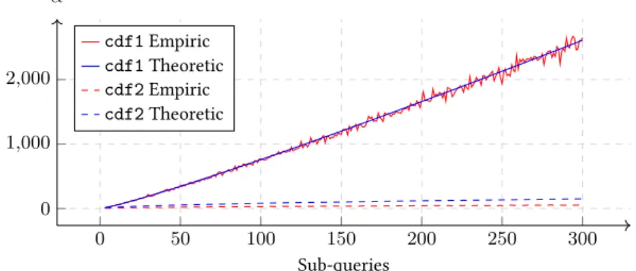
0 50 100 150 200 250 300 0 1,000 2,000 Sub-queries α cdf1Empiric cdf1Theoretic cdf2Empiric cdf2Theoretic

Figure 3:Error comparison (95% confidence)

So, the data analyst would know that usingcdf2in this case would

give, likely, a lower error. One can also use DPella to show a comparison betweencdf1andcdf2in terms of error when we keep the privacy

parameter fixed and we change the number of bins, wherecdf2gives

a better error when the number of bins is large [37] as illustrated in Figure 3. In the figure, we also show the empirical error to confirm that our estimate is tight—the oscillations on the empiricalcdf1are given

by the relative small (300) number of experimental runs we consider. Now, what if the data analyst choose to usecdf2because of what

we discussed before but she realizes that she can afford an errorα650;

what would be then the epsilon that gives suchα? One of the feature

of DPella is that the analystcan write a simple program that finds it by repetitively callingaccuracywith different epsilons—this is one of the

advantages of providing a programming framework. These different use cases shows the flexibility of DPella for different tasks in private data analyses.

(27)

2

Privacy

DPella is designed to help data analysts to have an informed deci-sion about how to spend their budget based on exploring the trade-offs between privacy and accuracy. In this section, we introduce DPella’s primitives and design principles responsible to ensure differential pri-vacy of queries written by data analysts.

2.1 Components of the API

Figure 4 shows part of DPella API. DPella introduces two abstract data types to respectively denote datasets and queries:

dataDatas r -- datasets

dataQuerya -- queries

The attentive reader might have observed that the API also introduces the data type Value a. This type is used to capture values resulting

from data aggregations. However, we defer its explanation for Section 3 since it is only used for accuracy calculations—for this section, readers can consider the typeValue aas isomorphic to the typea. It is also

worth noticing that the API enforces an invariant by construction:it is not possible to branch on results produced by aggregations—observe that there is no primitive capable to destruct a value of typeValuea. While

it might seem restrictive, it enables to write counting queries, which are the bread and butter of statistical analysis and have been the focus of the majority of the work in DP. Section 6 discusses, however, how to lift this limitation for specific analyses.

Values of typeDatas rrepresent sensitive datasets with accumu-lated stabilitys, where each row is of typer. Accumulated stability, on

(28)

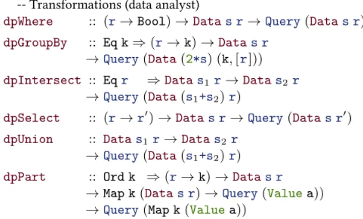
-- Transformations (data analyst)

dpWhere :: (r→Bool)→Datas r→Query(Datas r)

dpGroupBy :: Eq k⇒(r→k)→Datas r

→Query(Data(2*s) (k,[r]))

dpIntersect :: Eqr ⇒Datas1r→Datas2r

→Query(Data(s1+s2)r)

dpSelect :: (r→r0)→Datas r→Query(Datas r0)

dpUnion :: Datas1r→Datas2r

→Query(Data(s1+s2)r)

dpPart :: Ord k ⇒(r→k)→Datas r

→Map k(Datas r)→Query(Valuea))

→Query(Map k(Valuea)) -- Aggregations (data analyst)

dpCount:: Stbs ⇒→Datas r→Query(ValueDouble)

dpSum :: Stbs ⇒→Range a b→(r→Double)→Datas r

→Query(ValueDouble)

dpAvg :: Stbs ⇒→Range a b→(r→Double)→Datas r

→Query(ValueDouble)

dpMax :: Eq a⇒→Responsesa→(r→a)→Data1r

→Query(Valuea) -- Budget

budget :: Querya→

-- Execution (data curator)

dpEval:: (Data1r→Query(Valuea))→[r]→→IO a

Figure 4:DPella API: Part I

i.e.,1,2, etc. Stability is a measure that captures the number of rows in the dataset that could have been affected by transformations like se-lection or grouping of rows. In DP research, stability is associated with dataset transformations rather than with datasets themselves. In order to simplify type signatures, DPella uses the type parametersin datasets

to represent the accumulated stability of the transformations for which datasets have gone through—as done in [19]. Different than, e.g., PINQ [38], one novelty of DPella is that it computes stabilitystaticallyusing Haskell’s type-system.

Values of typeQueryarepresentcomputations, or queries, that yield values of typea. TypeQuery a is a monad [41], and because of this,

computations of typeQueryaare built by two fundamental operations: return::a→Querya

(29)

2.2. Transformations

The operationreturn xoutputs a query that just produces the value xwithout causing side-effects, i.e., without touching any dataset. The

function(>>=)—calledbind—is used to sequence queries and their as-sociated side-effects. Specifically,qp>>=fexecutes the queryqp, takes

itsresult, and passes it to the functionf, which then returns a second

query to run. Some languages, like Haskell, provide syntactic sugar for monadic computations known asdo-notation. For instance, the program

qp₁ >>= (λx1 → qp2>>= (λx2 → return (x1,x2))), which performs

queriesqp₁andqp₂and returns their results in a pair, can be written

asdox1 ← qp1;x2 ← qp2;return (x1,x2)which gives a more

“im-perative” feeling to programs. We split the API in four parts: transfor-mations, aggregations, budget prediction, and execution of queries—see next section for the description of API’s accuracy components. The first three parts are intended to be used by data analysts, while the last one is intended to beonlyused by data curators4.

2.2 Transformations

The primitivedpWhere filters rows in datasets based on a predicate functions (r→ Bool). The created query (of typeQuery (Data s r))

produces a dataset with the same row typerand accumulated stabilitys

as the dataset given as argument (Datas r). Observe that if we consider

two datasets which differ insrows in two given executions, and we apply

dpWhereto both of them, we will obtain datasets that will still differ in

srows—thus, the accumulated stability remains the same. The primitive

dpGroupByreturns a dataset where rows with the same key are grouped together. The functional argument (of typer→k) maps rows to keys

of typek. The rows in the return dataset (Data(2*s) (k,[r])) consist of key-rows pairs of type(k,[r])—syntax[r]denotes the type of lists of elements of typer. What appears on the left-hand side of the symbol⇒

are type constraints. They can be seen as static demands for the types appearing on the right-hand side of⇒. Type constraintEq kdemands

typek, denoting keys, to support equality; otherwise grouping rows

with the same keys is not possible. The accumulated stability of the new dataset is multiplied by2in accordance with stability calculations for transformations [38, 19]—observe that2*sis a type-level multiplication

done by a type-level function (or type family [20]) *. Our API also

considers transformations similar to those found in SQL like intersection 4_{A separation that can be enforced via Haskell modules [55]}

(30)

(dpIntersect), union (dpUnion), and selection (dpSelect) of datasets, where the accumulated stability is updated accordingly. Providing a general join transformation is known to be challenging [38, 43, 9, 30]. The output of a join may contain duplicates of sensitive rows, which makes difficult to bound the accumulated stability of datasets. However, and similar to PINQ, DPella supports a limited form of joins, where a limit gets imposed on the number of output records mapped under each key in order to obtain stability. For brevity, we skip its presentation and assume that all the considered information is contained by the rows of given datasets.

2.3 Partition

PrimitivedpPartdeserves special attention. This primitive is a mixture of a transformation and aggregations since it partitions the data (transfor-mation) to subsequently apply aggregations on each of them. More specif-ically, it splits the given dataset (Datas r) based on a row-to-key

map-ping (r→k). Then, it takes each partition for a given keykand applies

it to the corresponding functionDatas r→Query(Valuea), which is given as an element of a key-query mapping (Map k((Datas r)→

Query(Valuea))). Subsequently, it returns the values produced at ev-ery partition as a key-value mapping (Query(Map k(Valuea))). The primitivedpPartRepeat, used by the examples in Section 1, is imple-mented as a special case ofdpPartand thus we do not discuss it further. Partition is one of the most important operators to save privacy budget. It allows to run the same query on a dataset’s partitions but only paying for one of them—recall Theorem 3. The essential assumption that makes this possible is that every query runs ondisjoint datasets. Unfortunately, data analysts could ignore this assumption when writing queries.

To illustrate this point, we present the code in Figure 5. Queryq

pro-duces an-DP histogram of the colors found in the argumentdataset,

which rows are of typeColorand variablebinsenumerates all the

pos-sible values of such type. The code partitions the dataset by using the functionid::Color → Color (line 2) and executes the aggregation

counting query (dpCount) in each partition (line 3)—functionfromList

creates a map from a list of pairs. The attentive reader could notice that

dpCountis applied to the originaldatasetrather than the partitions.

(31)

2.4. Aggregations

1 q::→[Color]→Data1Double→Query(Map Color Double) 2 qeps bins dataset=dpPartid dataset dps

3 wheredps=fromList[(c, λds→dpCounteps dataset) 4 --dps=fromList[(c, λds→dpCounteps ds

5 |c←bins]

Figure 5:DP-histograms by usingdpPart

when estimating the required privacy budget. A correct implementation consists on executingdpCounton the corresponding partition as shown

in the commented line 4.

To catch coding errors as the one shown above, DPella deploys an static information-flow control (IFC) analysis similar to that provided by MAC [51]. IFC ensures that queries run bydpPartdo not perform queries on shared datasets by attaching provenance labels to datasets Datas rindicating to which part of the query they are associated with

and propagates that information accordingly.

Coming back to our previous example (see Figure 5), the IFC analysis will assign the provenance of datasetinqto the top-level fragment

of the query rather than to sub-queries executed in each partition—and DPella will raise an error at compile time whendsis accessed by the

sub-queries! Instead, if we comment line 3 and uncomment line 4, the queryqwill be successfully run by DPella (when there is enough privacy

budget) since every partition is only accessing their own partitioned data (denoted by variableds).

The implemented IFC mechanism istransparentto data analysts and curators, i.e., they do not need to understand how it works. Analysts and curators only need to know that, when the IFC analysis raises an alarm, is due to a possibly access to non-disjoint datasets when usingdpPart.

2.4 Aggregations

DPella presents primitives to count (dpCount), sum (dpSum), and

aver-age (dpAvg) rows in datasets. These primitives take an argumenteps::,

a dataset, and build a Laplace mechanism which iseps-differentially

pri-vate from which a noisy result gets return as a term of typeValueDouble.

The purpose of data typeValueais two fold: to encapsulate noisy

(32)

informa-tion about its accuracy—intuitively, how “noisy” the value is (explained in Section 3). The injected noise of these queries gets adjusted depend-ing on three parameters: the value of type, the accumulated stability of

the datasets, and the sensitivity of the query (recall Definition 2). More

specifically, the Laplace mechanism used by DPella uses accumulated sta-bilitysto scale the noise, i.e., it considerbfrom Theorem 1 asb=s·∆Q

. The sensitivity of DPella’s aggregations are either hard-coded into the implementation—similar to what PINQ does—or calculated statically. The sensitivities ofdpSumanddpAvgare determined by the range of

the values under consideration e.i., for the indicatedRange a b, the

sen-sitivity is computed asb-a. This is enforced by applying a clipping

func-tion (r→Double). This function ensures that the values under scrutiny

fall into the interval[a, b]before (and, fordpAvg, after) executing the

query. The sensitivity ofdpCountanddpMaxis set to1. To implement

the Laplace mechanism, the type constrainStbsindpCount,dpSum,

anddpAvgdemands the accumulated stability parametersto be a

type-level natural number in order to obtain a term-type-level representation when injecting noise. Finally, primitivedpMaximplements report-noisy-max

[15]. This query takes a list of possible responses (Responsesais a type

synonym for[a]) and a function of typer→ato be applied to every

row. The implementation ofdpMaxadds uniform noise to every score—

in this case, the amount of rowsvotingfor a response—and returns the responsewith the highest noisy score. This primitive becomes relevant to obtain the winner option in elections without singling out any voter. However, it requires that the accumulated stability of the dataset to be1 in order to be sound [8]. DPella guarantees such requirement by typing: the type of the given dataset as argument isData1r.

2.5 Privacy budget and execution of queries

The primitivebudgetstatically computes how much privacy budget

is required to run a query. It is worth notice that DPella returns an upper bound of the required privacy budget rather than the exact one— an expected consequence of using a type-system to compute it and provide early feedback to data analysts. Finally, the primitivedpEval is used by data curators to run queries (Querya) under given privacy

budgets (), where datasets are just lists of rows ([r]). It assumes that

the initial accumulated stability as1(Data 1 r) since the dataset has

(33)

2.6. Implementation

calculate the accumulated stability for datasets affected by subsequent transformations via the Haskell’s type system. This primitive returns a computation of typeIO a, which in Haskell are computations responsible

to perform side-effects—in this case, obtaining randomness from the system in order to implement the Laplace mechanism.

2.6 Implementation

DPella is implemented as a deep embedded domain-specific language (EDSL) in Haskell. Due to such design choice, data analysts can piggyback on Haskell’s infrastructure to build queries in a creative way. For instance, it is possible to leverage on any of Haskell’s pure functions. The following one-liner (of typeQuery[ValueDouble]) shows how to write a query that generates possibly non-disjoint datasets fromds::Datas rbased

on different criteria for then performing a counting.

mapM(flipdpSelectds>=>dpCounteps)fs

Variableepsis the epsilon to spend in each counting whilefs:: [r →

Bool]is the criteria list. The high-order functionsflip,mapM, and(>=>) are standard in Haskell and represent a function who switches arguments, the monadic versions ofmap, and the Kleisli arrow, respectively. Despite

DPella being a first-order interface, data analysts can use Haskell’s high-order functions to compactly describe queries.

(34)

3

Accuracy

DPella uses the data typeValuearesponsible to store a result of

typeaas well as information about its accuracy. For instance, a term of

typeValueDoublestores a noisy number (e.g., coming from executing

dpCount) together with its accuracy in terms ofa bound on the noise introduced to protect privacy.

DPella provides an static analysis capable to compute the accuracy of queries via the following function

accuracy::Query(Valuea)→β→α

which takes as an argument a query and returns a function, calledinverse Cumulative Distribution Function(iCDF), capturing the theoretical error

α for a given confidence1-β. Function accuracydoes not execute

queries but rather symbolically interpret all of its components in order to compute the accuracy of the result based on the sub-queries and how data gets aggregated. DPella follows the principle of improving accuracy calculations by detecting statistical independence. For that, it implements taint analysis [53] in order to track if values were drawn from statistically independent distributions.

3.1 Accuracy calculations

DPella starts by generating iCDFs at the time of running aggregations based on the following known result of the Laplace mechanism: Definition 3.1.1 (Accuracy for the Laplace mechanism).Given a randomized queryQ˜(·) : db→_Rimplemented with the Laplace mecha-nism as in Theorem 1, we have that

Prh|Q˜(D)−Q(D)|>log(1/β)·∆Q

i

(35)

3.1. Accuracy calculations

-- Accuracy analysis (data analyst)

accuracy::Query(Valuea)→β→α

-- Norms (data analyst)

norm∞:: [ValueDouble]→Value[Double]

norm2 :: [ValueDouble]→Value[Double]

norm1 :: [ValueDouble]→Value[Double]

rmsd :: [ValueDouble]→Value[Double] -- Accuracy combinators (data analyst)

add :: [ValueDouble]→ValueDouble neg ::ValueDouble→ValueDouble

Figure 6:DPella API: Part II

Recall that the Laplace mechanism used by DPella utilizes accumu-lated stabilitysto scale the noise, i.e., it considerbfrom Theorem 1 as b=s·∆Q

. Consequently, DPella stores the iCDFλβ→log(1/β)·s· ∆Q

for the values of typeValue Doublereturned by aggregation

primi-tives likedpCount,dpSum, anddpAvg. However, queries are often more

complex than just calling aggregation primitives—as shown byCDF2in

Figure 2b. In this light, DPella provides combinators responsible to ag-gregate noisy values, while computing its iCDFs based on the iCDFs of the arguments. Figure 6 shows DPella API when dealing with accuracy.

3.1.1 Norms

DPella exposes primitives to aggregate the magnitudes of several er-rors predictions into asinglemeasure—a useful tool when dealing with vectors. Primitivesnorm∞,norm2, and norm1 take a list of values of

typeValueDouble, where each of them carries accuracy information,

and produces asingle value(or vector) that contains a list of elements (Value[Double]) whose accuracy is set to be the well-known`∞-,`2-, `1-norms, respectively. Finally, primitivermsdimplements root-mean-square deviationamong the elements given as arguments. In our exam-ples, we focus on usingnorm∞, but other norms are available for the

taste, and preference, of data analysts.

3.1.2 Adding values

The primitiveaddaggregates values and, in order to compute accuracy of the addition, it tries to apply the Chernoff bound if all the values are

(36)

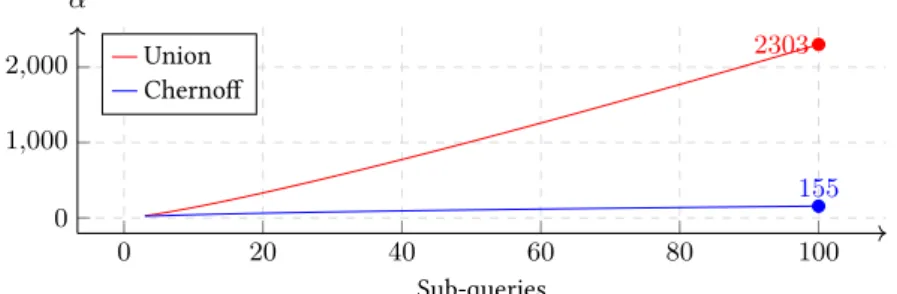
0 20 40 60 80 100 0 1,000 2,000 2303 155 Sub-queries α Union Chernoff

Figure 7:Union vs. Chernoff bounds

statistically independent; otherwise, it applies the union bound. More precisely, for the next definitions we assume that primitiveaddreceives

ntermsv1::ValueDouble,v2::ValueDouble, ... ,vn::ValueDouble.

Importantly, since we are calculating the theoretical error, we should consider random variables rather than specific numbers. The next defi-nition specifies howaddbehaves when applying union bound.

Definition 3.1.2 (add using union bound). Given n > 2 random variablesVj with their respectiveiCDFj, wherej ∈ 1. . . n, andαj =

iCDFj(β_n), then the additionZ =Pnj=1Vj has the following accuracy: Pr[|Z|>Pn

j=1αj]6β (4)

Observe that to compute theiCDFofZ, the formula uses theiCDFs

from the operands applied to β

n. Union bound makes no assumption about the distribution of the random variablesVj.

In contrast, the Chernoff boundoftenprovides a tighter error estima-tion than the commonly used union bound when adding several statisti-cally independentqueriessampled from a Laplace distribution. To illus-trate this point, Figure 7 shows that difference for thecdf2function we

presented in Section 1 with= 0.5(for each DP sub-query) andβ= 0.1. Clearly, the Chernoff bound is asymptotically much better when estimat-ing accuracy, while the union bound works best with a reduced number of sub-queries—observe how lines get crossed in Figure 7. In this light, and when possible, DPella computes both union bound and Chernoff bound and selects the tighter error estimation. However, to apply Cher-noff bound, DPella needs to be certain that the events are independent. Before explaining how DPella detects that, we give an specification of the formula we use for Chernoff.

(37)

3.1. Accuracy calculations

Definition 3.1.3 (addusing Chernoff bound [12]).Givenn>2 in-dependent random variablesVj ∼Lap(0, bj), wherej∈1. . . n,bM =

max {bj}j=1...n, andν > max{

q

Pn

j=1b2j, bM

q

ln_β2}, then the addi-tionZ =Pn

j=1Vj has the following accuracy:

Pr[|Z|> ν·q8 ln_β2]6β (5)

DPella uses the valueν =max{qPn

j=1b2j, bM

q

ln_β2}+0.00001to satisfy the conditions of the definition above when applying the Chernoff bound—any other positive increment to the computed maximum works as well5_.

Lastly, to support subtraction, DPella provides primitiveneg respon-sible to change the sign of a given value. We next explain how DPella checks that values come from statistically independent sampled vari-ables.

3.1.3 Detecting statistical independence

To detect statistical independence, we apply taint analysis when con-sidering terms of typeValuea. Specifically, every time a result of type

ValueDoublegets generated by an aggregation query in DPella’s API

(i.e.,dpCount,dpSum, etc.), it gets assigned a label indicating that it is

untaintedand thus statistically independent. The label also carries in-formation about the scale of the Laplace distribution from which it was sampled—a useful information when applying Definition 3.1.3. When the primitive addreceives all untainted values as arguments, the ac-curacy of the aggregation is determined by the best estimation pro-vided by either the union bound (Definition 3.1.2) or the Chernoff bound (Definition 3.1.3). Importantly, values produced byaddare considered tainted since they depend on other results. Whenadd receives any tainted argument, it proceeds to estimate the error of the addition by just using union bound. As an example, Figure 8 presents the query plan

totalCountwhich adds the results of hundreddpCountqueries over

different datasets, namelyds1,ds2,. . .,ds100. (The...denotes code

intentionally left unspecified.) The code calls the primitiveaddwith 5_{There are perhaps other ways to compute the Chernoff bound for the sum of} independent Laplace distributions, changing this equation in DPella does not require major work.

(38)

1 totalCount::Query(ValueDouble) 2 totalCount=do 3 v1 ←dpCount0.3 ds1 4 v2 ←dpCount0.25ds2 5 ... 6 v100←dpCount0.5 ds100 7 return(add[v1,v2,..., v100])

Figure 8:Combination of sub-queries results

the results of callingdpCount. (We use [x1, x2, x3]to denote the list

with elementsx1,x2, andx3.) What would it be then the theoretical

er-ror oftotalCount? The accuracy calculation depends on whether all

the values are untainted in line 7. When no dependencies are detected betweenv1,v2,. . .,v100, namely all the values are untainted, DPella

applies Chernoff bound in order to give a tighter error estimation. In-stead, for instance, ifv3was computed as an aggregation ofv1andv2,

e.g.,letv3=add[v1,v2], then line 7 applies union bound sincev3 is a

tainted value. With taint analysis, DPella is capable to detect dependen-cies among terms of typeValueDouble, and leverages that information

to apply different concentrations bounds.

In the next Section, we proceed to formally define our accuracy analysis.

3.2 Implementation

The accuracy analysis consists on symbolically interpreting a given query, calculating the accuracy of individual parts, and then combining them using our taint analysis. We introduce two polymorphic symbolic values:D::Data s randS[iCDF, s,ts] ::Value a. Symbolic dataset

Drepresents concrete datasets arising from data transformations. A

symbolic valueS[iCDF, s,ts]represents concrete values with tagsts

and aiCDFwhich is computed assuming a noise scales. Tags are used

to detect the provenance of symbolic values and when they arise from differentnoisy sources.

Functionaccuracytakes queries producing results of typeValuea.

Such queries are essentially built by performing data aggregation queries (e.g.,dpCount) preceded by a (possibly empty) sequence of other

(39)

primi-3.2. Implementation

tives like data transformations6_{. Figures 9 and 10 show the interesting}

parts of our analysis. Given awell-typed queryq::Query (Valuea),

accuracyq=iCDFwhereqBS[iCDF, s,ts]for somesandts. The

rules in 9 are mainly split into two cases: considering data aggregation queries and sequences of primitives glued together with(>>=).

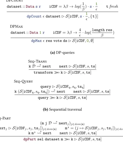
DPCount

dataset::Datas r iCDF=λβ→log(1

β)·s·

1

tfresh

dpCountdatasetBS[iCDF,s·1

,{t}]

DPMax

dataset::Data1r iCDF=λβ→4

·log(

length res

β )

dpMaxres vote dsBS[iCDF,0,∅]

(a)DP-queries

Seq-Trans

kD ∗next nextBS[iCDF, s,ts]

transform>>=kBS[iCDF, s,ts] Seq-Query

queryBS[iCDFq, sq,tsq] k(S[iCDFq, sq,tsq])

∗

next nextBS[iCDF, s,ts]

query>>=kBS[iCDF, s,ts]

(b)Sequential traversal

Seq-Part

(m jD ∗nextj)j∈dom(m)

(nextjBS[iCDFj, sj,tsj])j∈dom(m) m’= (j7→ S[iCDFj, sj,tsj])j∈dom(m)

k m’ ∗next nextBS[iCDF, s,ts]

dpPartsel dataset m>>=kBS[iCDF, s,ts]

(c)Accuracy calculation when partitioning data

Figure 9:Accuracy analysis implemented byaccuracy

6_{We ignore the case of}_{return val}_::_Query ₍_Value _a₎_{since the definition of}

(40)

The symbolic interpretation ofdpCount is captured by rule

DP-Count—see Figure 9a. This rule populates theiCDFof the return

sym-bolic value with the corresponding error calculations for Laplace as pre-sented in Definition 3.3.2 (with the scale adjusted with the accumulated stability). Observe that it extracts the stability information from the type of the considered dataset (ds::Datas r) and attaches a fresh tag

indi-cating an independently generated noisy value. The symbolic interpre-tation ofdpSumanddpAvgproceeds similarly todpCountand we thus

omit them for brevity.

Rule DPMax shows the symbolic interpretation ofdpMax whose

iCDFaligns with the one appearing in [8]. Observe that the return value

is tainted. The reason for that relies in the fact that the result, which is one of the responses inres, contains no noise—it is rather the process

that lead to determining the winning response which has been “noisy.” In this light, no scale of noise nor distribution can be associated to the response—as we did, for instance, withdpCount.

To symbolically interpret a sequence of primitives, the analysis gets further split into two cases depending if the first operation to interpret is a transformation or an aggregation, respectively—see Figure 9b. Rule Seq-Trans considers the former, wheretransformcan be any of the

transformation operations in Figure 4. It simply uses the symbolic value

Dto pass it to the continuationk. It can happen thatkDdoes not match

(yet) any part of DPella’s API required for our analysis to continue 7_.

However, the EDSL nature of DPella makes Haskell’s to reducekDto the

nextprimitive to be considered, which we capture askD ∗ next—and

we know that it will occur thanks to type preservation. We represent ( ∗_{) to pure reduction(s) in the host language like function application,} pair projections, list comprehension, etc. The analysis then continues symbolically interpreting thenextyield instruction. Rule Seq-Query

computes the corresponding symbolic value for the aggregationquery.

The symbolic value is then passed to the continuation, and the analysis continues with thenextyield instruction.

Rule Seq-Part shows the symbolic interpretation ofdpPart. The argumentm::Map k (Data s r → Query (Value a))describes the queries to execute once given the corresponding bins. Since these queries produce values, we need to symbolically interpret each of them to obtain their accuracy estimations. The rule applies each of those queries to a 7_{For instance,} _k _D _{= (}_λx _→ _dpCount ₁ _x₎ _D_{, and thus} ₍₍_λx _→

(41)

3.2. Implementation

symbolic dataset (m jD) 8. The symbolic values yield by each bin are

collected into the mappingm’, which is then passed to continuationk

in order to continue the analysis on thenextyield instruction.

3.2.1 Concentration Bounds

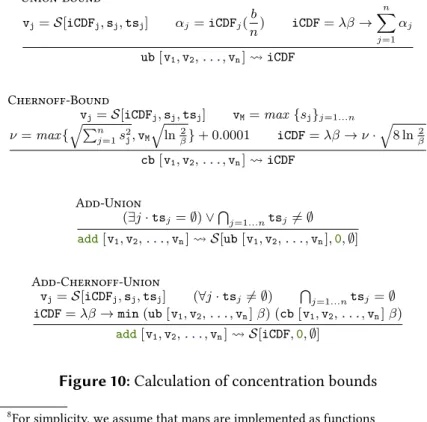
Figure 10 shows the part of our analysis responsible to apply concentra-tion bounds. Rules Union-Bound and Chernoff-Bound define pure functions (reduction ) which produce the concentration bounds as described in Definitions 3.1.2 and 3.1.3, respectively. We define the func-tion addbased on two cases. Rule Add-Union produces a symbolic value with aiCDFgenerated by the union bound (ub[v1,v2,...,vn]).

The symbolic value is tainted, which is denoted by the empty tags (∅).

The scale0 denotes that the scale of the noise and its distribution is unknown—adding Laplace distributions do not yield a Laplace distribu-tion. (However, the situation is different with Gaussians, see Section 3.3)

Union-Bound vj=S[iCDFj,sj,tsj] αj=iCDFj( b n) iCDF=λβ→ n X j=1 αj ub[v1,v2,...,vn] iCDF Chernoff-Bound vj=S[iCDFj,sj,tsj] vM=max{sj}j=1...n ν=max{qPn j=1s2j,vM q ln2 β}+ 0.0001 iCDF=λβ→ν· q 8 ln2 β cb[v1,v2,...,vn] iCDF Add-Union (∃j·tsj=∅)∨T_j₌₁_...ntsj6=∅ add[v1,v2,...,vn] S[ub[v1,v2,...,vn],0,∅] Add-Chernoff-Union vj=S[iCDFj,sj,tsj] (∀j·tsj6=∅) T_j₌₁_...ntsj=∅ iCDF=λβ→min(ub[v1,v2,...,vn]β) (cb[v1,v2,...,vn]β) add[v1,v2,...,vn] S[iCDF,0,∅]

Figure 10:Calculation of concentration bounds 8_{For simplicity, we assume that maps are implemented as functions}

(42)

Norm-Inf

vj=S[iCDFj,sj,tsj] iCDF=λβ→max{|iCDFj( β n)|}j=1...n norm∞[v1,v2,...,vn] S[iCDFM,0,∅] Norm-1 vj=S[iCDFj,sj,tsj] iCDF=λβ→ n X j=1 |iCDFj( β n)| norm1[v1,v2,...,vn] S[iCDF,0,∅]

Figure 11:Calculation of norms

This rule gets exercised when either the list of symbolic values con-tains a tainted one (∃j·tsj =∅) or have not been independently gener-ated (T

k=1...ntsj 6=∅). Differently, Add-Chernoff-Union produces a symbolic value with aiCDFwhich chooses the minimum error

estima-tion between union and Chernoff bound for a givenβ—sometimes union

bound provides tighter estimations when aggregating few noisy-values (recall Figure 7). This rule triggers when all the values are untainted (∀j·tsj 6= ∅) and independently generated (T_j₌₁_...ntsj =∅). At a first glance, one could believe that it would be enough to use the scale of the noise to track when values are untainted, i.e., if the scale is different from0, then the value is untainted. Unfortunately, this design choice is unsound: it will classify adding a variable twice as an independent sum: dox ←dpCountds;return(add[x, x]). It is also possible to con-sider various ways to add symbolic values to boost accuracy. We could easily write a pre-processing function which, for instance, firstly parti-tions the arguments into subset of independently generated values, ap-pliesaddto them (thus triggering Add-Chernoff-Union), and finally appliesaddto the obtained results (thus triggering Add-Union). The implementation of DPella enables to write such functions in a few lines of code.

3.2.2 Norms calculation

Figure 11 shows our static analysis when computingnorm∞andnorm1,

respectively. There is nothing special about the rules except to note that the results are symbolic values which are tainted. The reason for that is that norms are designed to condense (in one measure) the error of

(43)

3.3. Accuracy of Gaussian mechanism

the list of the arguments. By doing so, it is hard to assign an specific Laplace distribution with sensitivitysto the overall given vector. We

simply say that the return symbolic values are tainted—thus they can only be aggregated by Add-Union in Figure 10.

3.3 Accuracy of Gaussian mechanism

As aforementioned, DPella supports other notions of differential privacy— such as approximate differential privacy—together with the use of the Gaussian mechanism. Specifically, DPella supports a relaxation of the notion of differential privacy known as (, δ)-DP, formally defined as

follow.

Definition 3.3.1 ((, δ)-Differential Privacy[17]).A randomized query ˜

Q(·) : db→ _Rsatisfies(, δ)-differential privacy, with, δ>0, if and only if for any two datasetsD1andD2indb, which differ in one row, and

for every output setS ⊆Rwe have

Pr[ ˜Q(D1)∈S]6ePr[ ˜Q(D2)∈S] +δ (6)

The main difference between this notion of privacy and the one described in Theorem 1 is that (, δ)-DP introduces the probability mass δ that, intuitively, offers a probabilistic notion of privacy loss. More

concretely, (, δ)-DP ensures that for all adjacent datasets, the absolute

value of the privacy loss will be bounded bywith probability1−δ.

Observe that whenδ = 0, an (,0)-DP query satisfies pure-DP.

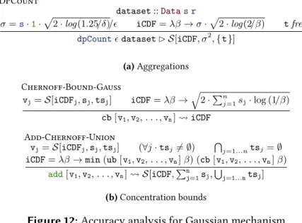
A standard implementation of (, δ)-DP queries is based on the

addi-tion of noise sampled from the Gauss distribuaddi-tion, this is, forQ: db→R an arbitrary function with sensitivity∆Q(as described in Definition 2) the Gaussian mechanism with parameterσadds noise scaled toN(0, σ2) to its output. When the noise to be added is calibrated in terms of,δ,

and∆Q, the Gaussian mechanism satisfies (, δ)-DP as stated on the

fol-lowing theorem.

Theorem 3.3.1 (Gaussian Mechanism [2]). For any , δ ∈ (0,1), the Gaussian output perturbation mechanism with standard deviation

σ =∆Q

q

2 log(1._δ25)/is(, δ)-differentially private

Similarly as with the Laplace mechanism, to provide bound estimates on the errors caused by the addition of Gaussian noise, DPella keeps track of Gauss’inverse Cummulative Distribution Function(iCDF). By following the general form of accuracy introduced in Definition 2, we have that: