Stock Price Prediction Using Sentiment Detection of Twitter

(1)

Stock Price Prediction Using Sentiment Detection of Twitter

C. Lee Fanzilli

March 18, 2015

Abstract

If Amazon can predict what books we want to read, Netflix can predict what movies we want to watch, and Google, if you are feeling lucky, can predict what we are looking for, then it wouldnt be farfetched to say that Twitter can predict what stocks we should buy. The prediction of stock trends based on this kind of data analysis have been a hot topic for some time now, because of the growth of social media and our technological advances in analyzing large amounts of data. With the development of various computing methods there have been studies [demonstrating that] computing techniques outperform conventional models in most cases [2]. The conventional investor, a long-term, rational person who picks stocks based on a companys history, board team, and projected performance, is now a bit of an anachronism. It is still true that past performance does not indicate future gains but we do know that individual stocks, and the market as a whole, are not 100% unpredictable. Cliff Asness provides some insight that the market is generally efficient, but not entirely so and that both market efficiency and human behavior move markets [4]. In particular, it is possible that new information is not incorporated into the stock price instantaneously. One source of such information may be tweets. We ask whether tweets about companies and their stock tickers, contain information that is not yet calculated into the price of the stock.

(2)

List of Figures

1 Figure one shows the structure of a tweet in .json format. . . 11 2 This figure shows how we would capture the effect of a tweet at time t on a given stock with

the open and closing prices of that stock for a certain time period. . . 15 3 Figure three shows a graph of the regression results for each stock, measuring if tweet

senti-ment follows stock returns. . . 19 4 Figure four shows a scatter plot of tweet sentiment against contemporaneous returns for each

stock. . . 21 5 Figure five shows a scatterplot for each stock using Twitter sentiment against future returns. 23

(4)

List of Tables

1 Table one shows the amount of times a particular stock was mentioned in the corpus of 281,000 tweets. . . 12 2 Table two shows a tweet from a given user about apple, each word and its corresponding

Sentiment Index, and the overall sentiment of the tweet. . . 13 3 Table three shows the table with computed sentiment index about a given tweet mentioning

a stock, with that stock ticker listed as well. . . 16 4 Table four shows the table for calculating the return of a stock on days that would be matched

up to tweet posts. . . 16 5 Table five shows the descriptive statistics of sentiment and contemporaneous returns for each

stock that we analyzed. . . 17 6 Table six shows the regression results for testing if Twitter sentiment follows stock returns. . 18 7 Table seven shows the regression results for testing if Twitter sentiment correlate to

contem-poraneous stock returns. . . 20 8 Table eight shows the regression results for testing if Twitter sentiment predicts future stock

(5)

1 Introduction

Intuition alone will not make anyone rich, nor will it even yield above-average returns. So we would like to find a more scientific way to judge this intangible about a stocks performance, the human behavioral aspect that might not already be factored into a stocks price. We cannot easily perform this analysis for every firm on the market, nor for the market as a whole, so instead we aim to find a relationship between new information contained in Twitter feeds and its influence on a selected number of individual companies. Traditional investors would gather fundamental information about a given stock, such as analyst reports, price earnings ratio, how much the company invests in research and development, how happy the compa-nys customers are, that stocks market capitalization, the quality of the product or service offered, as well as some other indicators to make predictions and decisions. None of this reflects sentiment; how buyers, customers, and the general public are feeling about a company, and whether that feeling can predict stock price movements. To perform this analysis, we will have to gather different types of data. The types of data we plan on using are Twitter posts gathered from Business Insiders top 101 tech tweeters, as well as techni-cal data collected from Yahoo [9]. We are collecting Twitter data because we know that stocks in the market are somewhat reactive to and influenced by new information. Since social media is the new frontier of fast emerging information, being able to utilize this type of data could prove to be extremely useful. And from recent behavioral finance studies, we know that emotions play a significant role in our decision-making as well [8].

So for this paper we would like to test whether mood and sentiment, as reflected in the tweets, can be used to predict movement in stock prices. In particular, we hypothesize that information contained in tweets is not immediately reflected in prices but rather tweets are forerunners of news that will reach the main body of investors only later. In order to complete this task, we plan on taking each tweet in our database related to a company with a listed stock, and calculate its sentiment index using the University of Pittsburghs MPQA Subjectivity Lexicon [7]. The MPQA Subjectivity Lexicon is a publicly-available lexicon which can be used to score words or phrases or fragments of words to determine whether they are positive or negative in the sentiment they express. There are many types of lexicons available but the MPQA version has been in existence for almost a decade and is well understood. In this lexicon there are over 8000 entries,

(6)

for each entry the lexicon produces a result to indicate if an entry is positive, neutral or negative in its sentiment. This is referred to as the prior polarity of a given word.

Using this lexicon as a basis for our analysis, we can create a sentiment index for each tweet based on the polarity of the words within it, so an example would be: @cwardzala released a new version with a bug... waiting for apple to roll back to the old one. In the subjectivity lexicon, the word bug has a negative polarity, thus indicating that this tweet is negative (since only that word appears in the lexicon), which seems fairly accurate. After this we will match up the days and time that a certain tweet is posted with the days and time of the price of the stock mentioned in the tweet. Then we will see if the subsequent movement in price is related to the polarity of the tweets.

2 Background and Related Work

Whenever someone tries to predict prices in the stock market, they must always consider the Efficient Market Hypothesis, or EMH [2]. The efficient market hypothesis states that it is impossible to beat the market because the efficiency of information flow in the modern stock market causes existing share prices to always incorporate and reflect all relevant information. From what we have read we found that the EMH is a very relevant hypothesis that has been tested for over 40 years. Eager entrepreneurs see the EMH as an old mans motto and that the real truth is the market can be beaten. We would characterize traditional buy-and-hold investors, such as the legendary Warren Buffet, as examples of EMH at its best. Buffet does not seem to contend to have an edge of any sort; rather, he has an investment strategy that is based upon a simple but not easy precept: analyze all existing information better than anyone else. I.E. EMH.

However, after reading numerous articles testing its validity we have come to the conclusion that there are times when EMH does not work quite as well as it should, especially in the short term. We call these dislocations of EMH. Granted, it is very rare to beat the stock market; but it can be done. We certainly know of times when stocks seemed to be overvalued; perhaps less famous are times when they seem to be undervalued, but both should be true if our hypothesis is correct. It is true that for every successful stock trader, there are thousands of failures, but with recent technological advancements and easy access to news and social media information we can make low risk, accurate assumptions about a particular stock. No

(7)

human can do this on his own though, extra computational power is necessary for anyone to attempt to tackle the amount of data required to understand more about a stock than EMH. Although a challenging task, many hedge funds and investment firms are able to produce consistent gains through the use of computer algorithms and big data analytics. We plan to show how feasible this task is for someone who is not a large hedge fund.

In Malkiels first paper on the EMH he discusses the validity of the Efficient Market Hypothesis and how at the start of the twenty-first century this hypothesis had become far less universal [5]. Many financial economists and statisticians started to believe that stock prices are at the very least partially predictable. Malkiel describes how psychologists in the behavioral finance field found that individuals, upon seeing a stock price rise, are then drawn into the market. This makes the assumption that people will continue to buy a particular stock until they deem the price too high. Malkiel makes a very valid point that while these assumptions may have some evidence to support them, there is not nearly enough to prove it. In the end, Malkiel concludes that other than some extremities like the 1999 bubble, the stock market is remarkably efficient. Luckily for us, 30 years later Malkiel continued his research on the EMH and wrote another paper concerning its true nature. In his second paper Malkiel shows whether or not the Efficient Market Hypothesis holds during long periods of time. He analyzed 355 equity funds from 1970 and measured their performance through December of 2003, a 33 year time span. Only 139 of these funds survived that long and when Malkiel graphed the results. He found that 20 of the 139 funds outperformed the S&P 500 (+15.24%) by 2% on average per year, or a gain of 17.24%. The other 119 either matched the S&P 500 or underperformed it. This is interesting because of all the funds that survived, the average total return per year was 13.42%, about 2% below the S&P 500 index [6]. He also notes that the record of the non-survivors up to their time of demise was substantially worse than the record of the survivors. So his research shows that there is hope in beating the market, but very little. Fortunately Twitter has not been around for 30 years so being able to beat the market may be more possible now than previously thought. One interesting fact to keep in mind is that in 2013, the Nobel Peace Prize was awarded to three economists who all had differing views on the EMH.

(8)

possible to predict market prices, based on other factors, but we must use computers to do so. There were several experiments ranging from stock market prediction using the utilization of Twitter data to mood and sentiment influence on human decision making. In Johan Bollens paper, Twitter mood predicts the stock market, he uses Twitter post sentiments about certain stocks to find a pattern between mood and the performance of a firms shares. Our emotions influence almost everything we do, when we are happy we want to do exciting things and when we are sad we often like to sulk and be alone and not take risk. So, we know that emotions, in addition to information, play a significant role in human decision-making, and what we want to find out is its role in financial decisions [3]. Social media generated data is important because it allows us to extract early indicators of a particular companys performance and perception in the market, well before the issuance of formal press releases or news reports. Since SEC filings are only released once per quarter, or when there is a reportable event, much information about a company must be derived from other means. By collecting and analyzing this socially generated data, we hope to get the investors edge in the market. Bollen makes it clear that a correlation does not mean causation, so he is not trying to prove that mood causes stocks to fluctuate but rather if they influence its fluctuation. What he found was that to a degree, sentiment does mirror performance, but with some variations. When testing the Dow Jones Industrial Average (DJIA), Bollen discovered that the major movements in the index correlate to the movements in Twitter moods on that given day. So on a day that the DIJA is doing well, we can see that the overall mood about those stocks on Twitter was high or positive. Nonetheless, it is not a perfect match, on some days the mood is low while the market is soaring. This indicates that there are other externalities at play that are influencing prices. This could of course be as simple as EMH taking the lead as opposed to more emotional investing.

Further influencing our research was another article we found regarding emotional influence on finan-cial decisions. This is important to our experiment because it shows how mood does in fact affect a persons behavior. One important point Olson made was that a number of empirical studies have found that mood influences reactions to risk, and risk plays a huge role in stock market decisions [8]. People always want to minimize risk and will typically take the safer route if they do not fully understand a given set of choices. This can be applied to financial decision because it shows how we humans are predictable, and if this is true

(9)

than it adds some predictability to stocks in the market. A recent example of this would be Tesla Motors. This company had been going sideways in the market for over three years. Then it received a lot of positive feedback from users of their cars as well as from financial analysts; the stock skyrocketed; it grew over ten fold in less than one year. The reason for this was a combination of positive publicity and news and a solid, reliable product. Tesla was not huge at the time, when compared to a company like Google which is highly valued, and the stock price was seen as too cheap for the type of company it was. So people began to buy, and buy, and buy, and now Tesla Motors is one of the more highly traded stocks on the market, and one of the most highly valued. Tesla, with a market capitalization of $30 billion, expects to sell about 40,000 cars in 2014. Ford, with a market capitalization of $60 billion, sold 180,000 cars in September 2014 alone. So, is Teslas market cap fuelled by EMH, where the markets think that Teslas superior products, R&D, marketing and so forth, will lead it to be the Ford of the future? Or is it really riding an emotional stock market roller coaster, with the stock price at the top of a coaster before a long drop?

In our research we will be looking at the sentiment index or mood of each tweet mentioning one of the particular stocks, from all 101 tweeters. We want to see if there is an indication of how a stock is doing when compared to Twitter sentiment. Well be checking to see if certain tweeters of the 101 have a greater or lesser influence when they tweet, as well as if multiple people tweet at the same time about the same stock; to verify if this has any more or less influence.

3 Data

In this section we will be discussing what data was needed to run our experiment. We will also go into detail on how we organized the data. For this experiment, we need three components: information on tweets, tweet sentiments, and stock prices. In the following subsections we will discuss how each was collected and utilized in this paper.

(10)

3.1 Twitter

Since we planned on working with Twitter data, we had to compile a list of people who would fit the criteria of active tweeters, with substantial followers, and an active role in the stock market. Luckily, Business Insider has a few lists of tweeters that they assembled based on different industries. Some notable people in this list are: Om Malik (founder of GigaOM), Julia Boorstin (CNBC journalist), Jack Dorsey (CEO of Square), Jeff Weiner (CEO of LinkedIn), and many others. We grabbed their list of top 101 tech tweeters, since the tech industry is fairly new and booming.

Twitter provides a python API which allows us to scrape the last 3200 tweets per user of the top 101 tweeters and convert them to json format. This file contains a list of each of the 3200 tweets of a user and includes the unique tweet ID, the user who posted, the time the tweet was posted, the physical text of the tweet, the amount of people who favorite that tweet, and the amount of retweets. The following image shows how tweets are structured in this format:

In Figure 1, we can see the tweet id is at the top which is unique for each entry, we can also view the text of the tweet, and in this case it is Hello, Saint Louis. Dinner on the Hill. The number of times the tweet was favorited (meaning someone liked it) and retweets (meaning someone tweeted that exact tweet) are also included further down. However, all we are interested in are the date, which is at the bottom, and the text. Using CouchDB (a free database by Apache) we uploaded every tweet we had, which came out to just over 281,000 total tweets [1]. The reason it wasn’t an even 320,000 was because not everyone on the list has tweeted 3200 or more times. We chose CouchDB as our main database because it has a python API, which is our choice of programming language for this experiment, and two very powerful map and reduce functions. We used a python module for CouchDB which allows us to create scripts that can access each tweet depending on what we want to extract from the data. Our next step was to look at tweets mentioning particular stocks. We chose AMD, GOOG, AAPL, BBRY, and MSFT for our experiment because of their popularity in the tech world. After some trial and error we were able to download a list of every tweet in our database that mentioned one of these stocks. Tweets that mention company name, stock symbol, company Twitter handle, or hashtags with either company name or stock symbol are all contained in the tweets that were filtered out for testing.

(11)

(12)

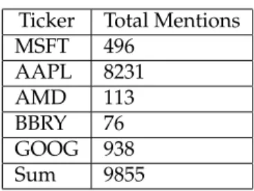
Ticker Total Mentions MSFT 496 AAPL 8231 AMD 113 BBRY 76 GOOG 938 Sum 9855

Table 1: Table one shows the amount of times a particular stock was mentioned in the corpus of 281,000 tweets.

From Table 1 we can see that AAPL had the most with 8231 mentions and BBRY had the least with only 76 mentions. In total these stocks were mentioned 9853 times out of 281,000 tweets. To put that into perspective, the total amount of tweets per day is around 500 million on average. Our dataset spans from about 2008/2009 to 2014 and only captures 281,000 tweets. We only have a tiny fraction of all tweets, and even with the amount that we have, only 3

3.2 Sentiment Detection

This section describes how we analyze sentiment of the text in a given tweet. There are many online databases for word sentiment, but from some of the papers we have read the MPQA subjectivity lexicon is a great open source corpus of English words with a corresponding sentiment index [7]. The University of Pittsburgh provides an MPQA subjectivity lexicon which contains a vast list of words and their corre-sponding sentiment, positive, negative, and neutral, based on that words typical use and part of speech. It is available for download, as a text document, on their website to anyone with an email address and a need for it. Using this lexicon we can create a script that analyzes each tweet, word for word, and will assign a sentiment value based on those words. Here is an example table we created by pulling tweets mentioning Apple and checking the sentiment polarity from the MPQA subjectivity lexicon for each word in a tweet. We then calculated an overall score based on the number of positive and negative words, defined by the MPQA lexicon, in the tweet:

(13)

Tweet MPQA SI Words Overall @cwardzala released a new version with a bug...

waiting for apple to roll back to the old one

Bug - negative negative

Handing out Groupon postcards in front of the ap-ple store on Michigan ave

Neutral neutral

I was about to make my first tweetstream-inspired purchase but the Marina apple store is sold out. #ipad

Neutral neutral

Final Cut Pro update restores many missing pro features: XSan, import/export XML, Media Stems track management, etc. apple.com/finalcutpro

Restore - positive positive

Steve Jobs has died. http://t.co/JUbLyMXb Remembrances are invited: remembering-steve@apple.com.

died - negative negative

RT @JasonLBaptiste: A share of $AAPL now costs as much as original iPod. If you bought Apple share instead then, it would be worth $27K today

original - positive, would - neutral, worth-positive, positive

RT @Street Insider: Apple $AAPL Holds Off On An-nouncing a Dividend http://t.co/POlPBWwx

neutral neutral

Rise and shine! Greetings from an Fran and the #apple #ipad event. Live on @foxbusiness and @FoxNews all day http://t.co/u29RQfee

shine - positive positive

Now showing off fanfare of grand central apple store opening. 362 retails stores open and 110m vis-itors in q4

fanfare - positive, open - positive positive

Table 2: Table two shows a tweet from a given user about apple, each word and its corresponding Sentiment Index, and the overall sentiment of the tweet.

(14)

From this table we hand pick some tweets mentioning Apple to see how accurate the lexicon is com-pared to our own intuition. For example, RT @JasonLBaptiste: A share of $AAPL now costs as much as original iPod. If you bought Apple share instead then, it would be worth $27K today. Within this tweet, the words original and positive come up as positive in the lexicon (so +2) and would come up neutral in the lexicon (+0), giving a score of 2 which indicates a positive sentiment. A negative example, @cwardzala released a new version with a bug... waiting for apple to roll back to the old one, which contains the word bug has a negative sentiment value in the lexicon (-1), indicating this is a negative tweet. Both examples are accurate when looking at the overall tweet, which is a good thing in this case. Next comes the good part.

3.3 Returns

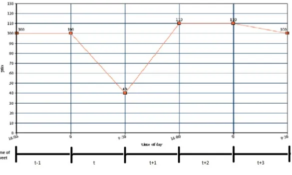
In this subsection we will explain how this data is used with stock price data so that we can run our regression analyses. For the regression we used the rate of return as the dependent variable and tweet sentiment as the independent variable. A good visual for what we are trying to test is:

(15)

Figure 2: This figure shows how we would capture the effect of a tweet at time t on a given stock with the open and closing prices of that stock for a certain time period.

The figure above illustrates the effect of twitter sentiment on future stock returns. For example, when a tweet is posted at time t, we want to see if there is a change in return at time t+1. In theory a positive tweet would influence positive future returns and a negative tweet would influence negative future returns, but this is what we aim to discover. RStudio was the program of choice for this part of the experiment, this is because of its ability to work well with excel files and econometric analysis. First we loaded up our sentiment data into RStudio, which was organized like this:

(16)

Tweet Date Posted Stock Mentioned Sentiment Index 1 Wed Oct 15 16:35:16 2014 MSFT +5

2 Thur Oct 16 18:20:00 2014 AAPL -2 3 Fri Oct 17 12:23:01 2014 GOOG 0

... ... ... ...

Table 3: Table three shows the table with computed sentiment index about a given tweet mentioning a stock, with that stock ticker listed as well.

Next we collected information on daily stock prices, including the close, open, high, low, and volume for each stock; which Yahoo Finance provides free of charge. We then uploaded this into RStudio to be merged with our tweet sentiment data since we want to see if a correlation between these two datasets exists. Unfortunately, the Twitter data is in Greenwich Mean Time and our stock price data is in Eastern Standard Time, so we had to normalize the time zones for comparison. However, we had to organize this table in a way such that the date of the tweet posted matches up with the opening price and closing price of that same day. If a tweet is posted during after hours, it would match up with the previous close and following open. This way we will be able to see if a correlation exists between tweet sentiment and returns. Once lined up and normalized our table looked like this:

Date and Time Price t Sentiment Price t+1 Returns 9/29/2008 9:30 23.06 -1 22.43 -0.027 9/17/2009 16:00 22.43 0 22.91 0.021 5/27/2010 9:30 22.91 0 21.59 -0.058 8/23/2010 16:00 21.59 0 21.59 0 8/23/2010 16:00 21.59 1 21.8 0.01

Table 4: Table four shows the table for calculating the return of a stock on days that would be matched up to tweet posts.

(17)

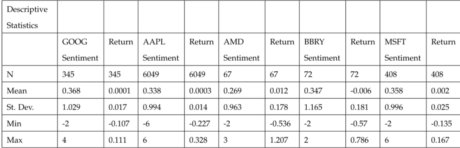
time t to the end of time t, or t+1. This represents mood sentiments effect on the return for this time period. Furthermore, below is a descriptive statistics table of our dataset showing the range in tweet sentiment and contemporaneous returns for each stock in our data.

Descriptive Statistics GOOG Sentiment Return AAPL Sentiment Return AMD Sentiment Return BBRY Sentiment Return MSFT Sentiment Return N 345 345 6049 6049 67 67 72 72 408 408 Mean 0.368 0.0001 0.338 0.0003 0.269 0.012 0.347 -0.006 0.358 0.002 St. Dev. 1.029 0.017 0.994 0.014 0.963 0.178 1.165 0.181 0.996 0.025 Min -2 -0.107 -6 -0.227 -2 -0.536 -2 -0.57 -2 -0.135 Max 4 0.111 6 0.328 3 1.207 2 0.786 6 0.167

Table 5: Table five shows the descriptive statistics of sentiment and contemporaneous returns for each stock that we analyzed.

The first thing we noticed about our descriptive statistics table was that the number of observations decreased from our table counting the number of mentions for each of the stocks. This is because tweets posted on days that there is no stock information, such as weekends, would not be captured by this model. It was also interesting to see the range in sentiment values for each stock, for instance Apples lowest sen-timent was -6 and its highest was 6, indicating that 6 words in a tweet were negative and 6 in another were positive. This was alarming at first so we checked to see if there had been an issue in calculating the sentiment, but each tweet did in fact have enough words to give them very low and very high values respectively. Unlike sentiment, the range in returns are fairly uniform for each stock. We can see that the difference between min and max return for each is around a 200-300% difference. However, the max return for AMD is 1.207, or a contemporaneous return of 120.7%, we checked this in our data and determined that in that time period, AMD price had risen from around 3 dollars per share to around 8 dollars per share, indicating an accurate calculation. With our data ready for testing, we began implementing our regressions.

(18)

4 Results

The results section is organized in the following way: first we will discuss if stock prices follow twitter sentiment, then if stock prices are correlated with twitter sentiment, and lastly if twitter sentiment predicts stock prices. In this section we discuss the results of our regressions. First we will present a table of our regressions and then graphs to accompany them.

4.1 Does Twitter sentiment follow prices?

In this subsection we analyze our regression of Twitter sentiment following past stock returns. Below we include a table of results from our analysis, which shows the correlation, number of observations, R-squared and adjusted R-squared, and standard error. Note that next to the coefficient are stars indicating level of significance of a variable, none means insignificant, one means slightly significant, and so on, with the maximum possible for this model being three stars. Underneath the coefficient the p-value is included in the regression table. A significance of the constant, or intercept, does not indicate any economic implication about the model.

Dependent Variable: Returns

GOOG AAPL AMD BBRY MSFT

Tweet Sentiment Coefficient -0.0001 (0.001) 0.0002 (0.0002) 0.003 (0.024) -0.014 (0.021) -0.001 (0.001) Constant Coefficient 0.0001 (-0.0001) 0.0003 (0.0002) 0.012 (0.024) -0.004 (0.023) 0.002* (0.001)

Observations 343 6047 65 70 406

R2 0.00002 0.0001 0.0002 0.006 0.001

Adj. R2 -0.003 -0.00005 -0.016 -0.008 -0.001

Std. Error 0.017 0.014 0.182 0.184 0.025

Table 6: Table six shows the regression results for testing if Twitter sentiment follows stock returns.

In RStudio we plotted the results of Twitter sentiment and past stock returns of our regression for each stock:

(19)

Figure 3: Figure three shows a graph of the regression results for each stock, measuring if tweet sentiment follows stock returns.

From the above regression table and scatterplots of tweet sentiment against returns, we can see that there is little to no correlation between the two variables. The slope coefficients for tweet sentiment are very low in each instance, all below 0.001, which indicates that as return increases or decreases, tweet sentiment does not follow a pattern. In addition to that, tweet sentiment is insignificant in following past returns according to our model, which is indicated in the low R-squared value and lack of significant stars. This shows that the sentiment of tweets about a given stock are not related to past returns, or in short, tweet sentiment about a stock does not follow that stocks returns.

(20)

4.2 Are prices correlated with Twitter sentiment?

In this subsection we analyze our regression of Twitter sentiment correlating to contemporaneous returns of a given stock. Our regression results for this model were not too different from the previous table, which was not surprising. Testing if tweet sentiment is correlated to contemporaneous returns was our baseline analysis for making sure our methods work properly. In order for there to be a correlation, a stocks price would need to react at the same time the tweet was posted and in a way that is comparable to the sentiment value. Ironically, we were pleased with the results of our regression analysis. Below is a table displaying our results:

Tweet Sentiment Coefficient 0.001 (-0.001) -0.0002 (0.0002) -0.023 (0.023) -0.013 (0.019) 0.001 (-0.001) Constant Coefficient -0.0003 (-0.001) 0.0004** (-0.0002) 0.018 (0.023) -0.002 (0.022) 0.002 (-0.001)

Observations 345 6049 67 72 408

R2 0.005 0.0002 0.016 0.007 0.001

Adj. R2 0.002 0.0001 0.001 -0.008 -0.001

Std. Error 0.017 0.014 0.178 0.182 0.025

Table 7: Table seven shows the regression results for testing if Twitter sentiment correlate to contempora-neous stock returns.

We then created a scatterplot of Twitter sentiment against contemporaneous returns with the results from our regression analysis:

(21)

Figure 4: Figure four shows a scatter plot of tweet sentiment against contemporaneous returns for each stock.

From the above regression table and scatterplots of tweet sentiment against contemporaneous returns, we can see that there is little to no correlation between the two variables. The slope coefficients for tweet sentiment are all below 0.01 in this model as well. We can see that tweet sentiment is not significant in accounting contemporaneous returns, and have a relatively low R-squared. However, before implementing this model we expected to see no correlation because stock prices cannot react at the same time a tweet is posted, it just is not possible. Regardless, it is still interesting to look at the variation in results for each stock. When looking at the scatterplots, there are some data points that look like obvious outliers (like with AMD) but after confirming that this was accurate, we kept it in the analysis. From the scatterplots we can also see that both BlackBerry and AMD have slightly negative slopes when compared to the other stocks,

(22)

but because tweet sentiment is not significant we cannot say that it is inversely related to contemporaneous returns.

4.3 Does Twitter Sentiment predict prices?

In this subsection we analyze our regression of Twitter sentiment prediction future returns of a given stock. This is where the experiment gets interesting. Our regression for this model had some interesting results compared to the two previous analyses. Unfortunately, the majority of our stocks did not show any signs of correlation between tweet sentiment and future returns. However, the results we saw with Google provided some useful insight. Below is a table of our regression results:

Tweet Sentiment Coefficient 0.003*** (0.001) -0.0003 (0.0003) -0.018 (0.036) 0.001 (0.001) 0.002 (0.002) Constant Coefficient -0.001 (0.001) 0.001*** (0.0004) 0.033 (0.033) 0.002 (0.001) 0.004*** (0.002

Observations 328 4252 70 36 356

R2 0.02 0.0001 0.004 0.001 0.003

Adj. R2 0.017 -0.0001 -0.011 -0.001 0.0003

Std. Error 0.02 0.022 0.248 0.025 0.037

Table 8: Table eight shows the regression results for testing if Twitter sentiment predicts future stock returns.

Below are scatterplots of Twitter sentiment against future returns for each given stock in our regression analysis:

(23)

Figure 5: Figure five shows a scatterplot for each stock using Twitter sentiment against future returns.

From the above regression table and scatterplots of tweet sentiment against future returns, we can see that there is little to no correlation between the two variables in most cases. However, with Google we can see that there is in fact a positive slope coefficient. In our regression table we can see that tweet sentiment of Google is indeed statistically significant 0.01 significance level. This implies that the sample on Google gives reasonable evidence to support that tweet sentiment can predict future returns, and our model has a less than 1% chance of being wrong. The slope coefficient of tweet sentiment is 0.003, which seems very small even if it is significant. This simply indicates that the data on Google is very spread out from the best-fit line. An important thing to notice though is that the adjusted R-squared value is quite low, illustrating that the relationship between tweet sentiment and future returns is rather weak. Having an adjusted R-squared value of 0.017 shows that tweet sentiment significantly captures 1.7% of the variability in future

(24)

returns around the mean. Although the value is small, this does not change the fact that tweet sentiment was significant in our analysis of future returns on Google. Since there is only one case in which there is any significance, we cannot say that it is definitely possible to predict future prices with Twitter sentiment. But, the fact that we found significance with Google does indicate that it could be possible.

5 Conclusion and Future Work

In conclusion we found that the relationship between stock price data and Twitter sentiment data are not likely correlated. We were sure that our analysis of tweet sentiment and past returns would give us some-thing significant because it makes sense that if Apple or Google started falling in price then people would get upset, and visa-versa with rising prices. However, our results showed otherwise. Instead it seems as though in all three result cases, tweet sentiment and returns are not related. This can be explained in a couple of ways. First, it is very possible that Twitter data could be captured in the market instead of what we originally thought. Compared to an article in the Wall Street Journal, Twitter allows as a faster median for spreading and receiving information. We also must also understand that tweets and stock prices are not directly related, when someone tweets about a company it is not AAPL prices are on the rise so we are basing it on other factors. Instead, we are basing it on other factors, like launches, product releases, or bugs in devices. So when someone tweets oh wow the apple watch is amazing, we are trying to capture information that influenced the stock price. Also, Twitter posts are generally not about the fundamentals of a company, but rather a persons opinion about that company or companys product. From these results we are able to consider that the EMH could be applied to our experiment, and that the public information on Twitter is indeed incorporated into stock prices. There are also other obstacles that we could not account for in our experiment, but may be remedied in future work.

First is the frequency of our data, we only have daily open and close price for a given stock which are pretty infrequent compared to Twitter posts. Because of this, we could only really look at two separate intervals of stock price on a given day, whereas hundreds of millions of tweets are posted throughout the day; not just at 9:00 AM EST and 4:30 PM EST. If we had stock price data by seconds instead, this would be much more useful given the type of data that we are using. Second, we do not have as much Twitter data

(25)

as other similar experiments. Others tend to have upwards of several million tweets while we have only around 281,000 tweets. Expanding the amount of stocks would also be a good idea, but also expanding the types of stocks we analyze would be even better. We only look at tech stocks and tech tweeters, but investigating other sectors could yield different results. Lastly, instead of just using return we would also include the abnormal returns, if we net out the market return we would be able to look at the overall market instead of just one particular stock. Calculating abnormal return would also give us a less noisy measure of return on individual stocks. Given an adequate dataset, we would also consider using more advanced tools of machine learning like Support Vector Machines because they are powerful at handling multi-dimensional data and are fairly popular in similar experiments. These improvements would allow us to make a more in depth analysis of the data, and possibly be able to put it into action and try to make some money.

References

[1] Apache. ”apache couchdb is a database.”.

[2] Clifford Asness, Andrea Frazzini, Ronen Israel, and Tobias J. Moskowitz. Fact, fiction and momentum investing.Forthcoming in the Journal of Portfolio Management. N.p., 9:2014, May 2014.

[3] J. Bollen, H. Mao, and X. J. Zeng. Twitter mood predicts the stock market. School of Informatics and Computing, Indiana University-Bloomington, 2010.

[4] B. Conway. AQR’s Cliff Asness on the Mostly-But-Not-Always Efficient Market. ¡Baron’s Blog, 2014.

[5] Burton G. Malkiel. The efficient market hypothesis and its critics. Journal of Economic Perspectives, 17(1):59–82, September 2014.

[6] Burton G. Malkiel. Reflections on the efficient market hypothesis: 30 years later. The Financial Review, 40(1):1–9, September 2014.

(26)

[8] K. R. Olson. A literature review of social mood.The Institute of Behavioral Finance ARTICLES A Literature Review of Social Mood, 7(4):193–203, 2006.

[9] Abby Yarow. Presenting: The 101 tech people you have to follow on twitter. Business Insider. May, 21:2012, November 2014.