Edinburgh Research Explorer
StreamApprox: Approximate Computing for Stream Analytics
Citation for published version:
Quoc, DL, Chen, R, Bhatotia, P, Fetzer, C, Hilt, V & Strufe, T 2017, StreamApprox: Approximate Computing
for Stream Analytics. in ACM/IFIP/USENIX Middleware 2017. ACM, pp. 185-197, 18th ACM/IFIP/USENIX
Middleware Conference, Las Vegas, United States, 11-15 December. DOI: 10.1145/3135974.3135989
Digital Object Identifier (DOI):
10.1145/3135974.3135989
Link:
Link to publication record in Edinburgh Research Explorer
Document Version:
Peer reviewed version
Published In:
ACM/IFIP/USENIX Middleware 2017
General rights
Copyright for the publications made accessible via the Edinburgh Research Explorer is retained by the author(s)
and / or other copyright owners and it is a condition of accessing these publications that users recognise and
abide by the legal requirements associated with these rights.
Take down policy
The University of Edinburgh has made every reasonable effort to ensure that Edinburgh Research Explorer
content complies with UK legislation. If you believe that the public display of this file breaches copyright please
contact [email protected] providing details, and we will remove access to the work immediately and
investigate your claim.
StreamApprox: Approximate Computing for Stream Analytics
Do Le Quoc
1, Ruichuan Chen
2, Pramod Bhatotia
3,
Christof Fetzer
1, Volker Hilt
2, Thorsten Strufe
1 1TU Dresden,2Nokia Bell Labs,3University of Edinburgh and Alan Turing Institute
Abstract
Approximate computing aims for efficient execution of workflows where an approximate output is sufficient instead of the exact output. The idea behind approximate computing is to compute over a representative sample instead of the entire input dataset. Thus, approximate computing — based on the chosen sample size — can make a systematic trade-off between the output accuracy and computation efficiency.
Unfortunately, the state-of-the-art systems for approximate com-puting primarily target batch analytics, where the input data re-mains unchanged during the course of computation. Thus, they are not well-suited for stream analytics. This motivated the design of StreamApprox— a stream analytics system for approximate com-puting. To realize this idea, we designed an online stratified reser-voir sampling algorithm to produce approximate output with rigor-ous error bounds. Importantly, our proposed algorithm is generic and can be applied to two prominent types of stream processing sys-tems: (1) batched stream processing such as Apache Spark Stream-ing, and (2) pipelined stream processing such as Apache Flink.
To showcase the effectiveness of our algorithm, we implemented StreamApprox as a fully functional prototype based on Apache Spark Streaming and Apache Flink. We evaluated StreamApprox using a set of microbenchmarks and real-world case studies. Our results show that Spark- and Flink-based StreamApprox systems achieve a speedup of 1.15×—3×compared to the respective native Spark Streaming and Flink executions, with varying sampling frac-tion of 80% to 10%. Furthermore, we have also implemented an improved baseline in addition to the native execution baseline — a Spark-based approximate computing system leveraging the exist-ing samplexist-ing modules in Apache Spark. Compared to the improved baseline, our results show that StreamApprox achieves a speedup of 1.1×—2.4×while maintaining the same accuracy level.
1
Introduction
Stream analytics systems are extensively used in the context of modern online services to transform continuously arriving raw data streams into useful insights [20,34,47]. These systems tar-get low-latency execution environments with strict service-level agreements (SLAs) for processing the input data streams.
In the current deployments, the low-latency requirement is usu-ally achieved by employing more computing resources and par-allelizing the application logic over the distributed infrastructure. Since most stream processing systems adopt a data-parallel pro-gramming model [17], almost linear scalability can be achieved with increased computing resources.
However, this scalability comes at the cost of ineffective utiliza-tion of computing resources and reduced throughput of the system. Moreover, in some cases, processing the entire input data stream would require more than the available computing resources to meet the desired latency/throughput guarantees.
To strike a balance between the two desirable, but contradic-tory design requirements — low latency and efficient utilization of computing resources — there is a surge ofapproximate computing paradigm that explores a novel design point to resolve this tension. In particular, approximate computing is based on the observation that many data analytics jobs are amenable to an approximate rather than the exact output [18,35]. For such workflows, it is possible to trade the output accuracy by computing over a subset instead of the entire data stream. Since computing over a subset of input requires less time and computing resources, approximate computing can achieve desirable latency and computing resource utilization.
To design an approximate computing system for stream analytics, we need to address the following three important design challenges: Firstly, we need an online sampling algorithm that can perform “on-the-fly” sampling on the input data stream. Secondly, since the input data stream usually consists of sub-streams carrying data items with disparate population distributions, we need the online sampling algorithm to have a “stratification” support to ensure that all sub-streams (strata) are considered fairly, i.e., the final sample has a representative sub-sample from each distinct sub-stream (stratum). Finally, we need an error-estimation mechanism to interpret the output (in)accuracy using an error bound or confidence interval.
Unfortunately, the advancements in approximate computing are primarily geared towards batch analytics [1,26,39], where the input data remains unchanged during the course of computation (see§8 for details). In particular, these systems rely on pre-computing a set of samples on the static database, and take an appropriate sample for the query execution based on the user’s requirements (i.e., query execution budget). Therefore, the state-of-the-art systems cannot be deployed in the context of stream processing, where the new data continuously arrives as an unbounded stream.
As an alternative, we could in principlerepurposethe available sampling mechanisms in Apache Spark (primarily available for machine learning in the MLib library [21]) to build an approximate computing system for stream analytics. In fact, as a starting point, we designed and implemented an approximate computing system for stream processing in Apache Spark based on the available sam-pling mechanisms. Unfortunately, as we will show later, Spark’s stratified sampling algorithm suffers from three key limitations for approximate computing, which we address in our work (see§4 for details). First, Spark’s stratified sampling algorithm operates in a “batch” fashion, i.e., all data items are first collected in a batch as Resilient Distributed Datasets (RDDs) [46], and thereafter, the actual sampling is carried out on the RDDs. Second, it does not handle the case where the arrival rate of sub-streams changes over time because it requires a pre-defined sampling fraction for each stratum. Lastly, the stratified sampling algorithm implemented in Spark requires synchronization among workers for the expensive join operation, which imposes a significant latency overhead.
To address these limitations, we designed anonline stratified
reservoir sampling algorithmfor stream analytics. Unlike existing Spark-based systems, we perform the sampling process “on-the-fly”
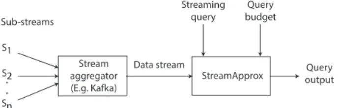
StreamApprox Data stream Stream aggregator (E.g. Kafka) Sub-streams S1 S2 Sn . . Query output Streaming query Query budget
Figure 1.System overview
to reduce the latency as well as the overheads associated in the process of forming RDDs. Importantly, our algorithmgeneralizes to two prominent types of stream processing models: (1) batched stream processing employed by Apache Spark Streaming [22], and (2) pipelined stream processing employed by Apache Flink [20].
More specifically, our sampling algorithm makes use of two tech-niques: reservoir sampling and stratified sampling. We perform reservoir sampling for each sub-stream by creating a fixed-size reservoir per stratum. Thereafter, we assign weights to all strata respecting their respective arrival rates to preserve the statistical quality of the original data stream. The proposed sampling algo-rithm naturally adapts to varying arrival rates of sub-streams, and requires no synchronization among workers (see §3).
Based on the proposed sampling algorithm, we designed StreamAp-prox, an approximate computing system for stream analytics (see Figure1). StreamApprox provides an interface for users to specify streaming queries and their execution budgets. The query execution budget can be specified in the form of latency guarantees or avail-able computing resources. Based on the query budget, StreamAp-prox provides an adaptive execution mechanism to make a sys-tematic trade-off between the output accuracy and computation efficiency. In particular, StreamApprox employs the proposed sam-pling algorithm to select a sample size based on the query budget, and executes the streaming query on the selected sample. Finally, StreamApprox provides a confidence metric on the output accu-racy via rigorous error bounds. The error bound gives a measure of accuracy trade-off on the result due to the approximation.
We implemented StreamApprox based on Apache Spark Stream-ing [22] and Apache Flink [20], and evaluate its effectiveness via various microbenchmarks. Furthermore, we also report our experi-ences on applying StreamApprox to two real-world case studies. Our evaluation shows that Spark- and Flink-based StreamApprox achieves a significant speedup of 1.15×to 3×over the native Spark Streaming and Flink executions, with varying sampling fraction of 80% to 10%, respectively.
In addition, for a fair comparison, we have also implemented an approximate computing system leveraging the sampling modules already available in Apache Spark’s MLib library (in addition to the native execution comparison). Our evaluation shows that, for the same accuracy level, the throughput of Spark-based StreamApprox is roughly 1.1×—2.4×higher than the Spark-based approximate computing system for stream analytics.
To summarize, we make the following main contributions. • We propose the online adaptive stratified reservoir sampling
(OASRS) algorithm that preserves the statistical quality of the input data stream, and is resistant to the fluctuation in the arrival rates of strata. Our proposed algorithm is generic
and can be applied to the two prominent stream processing models: batched and pipelined stream processing models. • We extend our algorithm for distributed execution. The
OASRS algorithm can be parallelized naturally without re-quiring any form of synchronization among distributed workers.
• We provide a confidence metric on the output accuracy using an error bound or confidence interval. This gives a measure of accuracy trade-off on the result due to the approximation.
• Finally, we have implemented the proposed algorithm and mechanisms based on Apache Spark Streaming and Apache Flink. We have extensively evaluated the system using a series of microbenchmarks and real-world case studies.
StreamApprox’s codebase with the full experimental evalua-tion setup is publicly available:https://streamapprox.github.io/. A detailed version of this paper is available as a technical report [37].
2
Overview and Background
This section gives an overview of StreamApprox, its computa-tional model, and the design assumptions. Lastly, we conclude this section with a brief background on the technical building blocks.
2.1 System Overview
StreamApprox is designed for real-time stream analytics. Figure1 presents the high-level architecture of StreamApprox. The input data stream usually consists of data items arriving from diverse sources. The data items from each source form asub-stream. We make use of a stream aggregator (e.g., Apache Kafka [24]) to com-bine the incoming data items from disjoint sub-streams. StreamAp-prox then takes this combined stream as the input for data analytics. We facilitate data analytics on the input stream by providing an interface for users to specify the streaming query and its cor-responding query budget. The query budget can be in the form of expected latency/throughput guarantees, available computing resources, or the accuracy level of query results.
StreamApprox ensures that the input stream is processed within the specified query budget. To achieve this goal, we make use of approximate computing by processing only a subset of data items from the input stream, and produce an approximate output with rigorous error bounds. In particular, StreamApprox uses a parallelizable online sampling technique to select and process a subset of data items, where the sample size can be determined based on the query budget.
2.2 Computational Model
The state-of-the-art distributed stream processing systems can be classified in two prominent categories:(i)batched stream process-ing model, and(ii)pipelined stream processing model.Our proposed
algorithm for approximate computing is generalizable to both stream processing models, and preserves their advantages.
Batched stream processing model.In this computational model, an input data stream is divided into small batches using a pre-defined batch interval, and each such batch is processed via a dis-tributed data-parallel job. Apache Spark Streaming [22] adopted this model to process input data streams.
Pipelined stream processing model.In contrast to the batched stream processing model, the pipelined model streams each data
Algorithm 1 Reservoir sampling algorithm Input:N←sample size
begin
r eservoir← ∅;//Set of items sampled from the input stream
foreacharriving itemxido if|r eservoir|<Nthen
//Fill up the reservoir r eservoir.append(xi); end
else p←N
i ;
//Flip a coin comes heads with probabilityp head←flipCoin(p);
ifheadthen
//Get a random index in the reservoir
j←getRandomIndex(0,|r eservoir| −1);
//Replace old item in reservoir byxi r eservoir[j]←xi
end end end end
item to the next operator as soon as the item is ready to be processed without forming the whole batch. Thus, this model achieves low latency. Apache Flink [20] implements this model to provide a truly native stream processing engine.
Note that both stream processing models support the time-based sliding window computation [6]. The processing window slides over the input stream, whereby the newly incoming data items are added to the window and the old data items are removed from the window. The number of data items within a sliding window may vary in accordance to the arrival rate of data items.
2.3 Design Assumptions
StreamApprox is based on the following assumptions. We discuss the possible means to address these assumptions in §7.
1. We assume there exists a virtual cost function which trans-lates a given query budget (such as the expected latency guarantees, or the required accuracy level of query results) into the appropriate sample size.
2. We assume that the input stream is stratified based on the source of data items, i.e., the data items from each sub-stream follow the same distribution and are mutually inde-pendent. Here, astratumrefers to one sub-stream. If multi-ple sub-streams have the same distribution, they are com-bined to form a stratum.
2.4 Background: Technical Building Blocks
We next describe the two main technical building blocks of StreamAp-prox: (a) reservoir sampling, and (b) stratified sampling.
Reservoir sampling.Suppose we have a stream of data items, and want to randomly select a sample ofNitems from the stream. If we know the total number of items in the stream, then the solution is straightforward by applying the simple random sampling [30]. However, if a stream consists of an unknown number of items or the stream contains a large number of items which could not fit into the storage, then the simple random sampling does not work and a sampling technique calledreservoir samplingcan be used [41].
Reservoir sampling receives data items from a stream, and main-tains a sample in a buffer calledreservoir. Specifically, the technique populates the reservoir with the firstNitems received from the stream. After the firstNitems, every time we receive thei-th item (i>N), we replace each of theN existing items in the reservoir with the probability of 1/i, respectively. In other words, we accept thei-th item with the probability ofN/i, and then randomly re-place one existing item in the reservoir. In doing so, we do not need to know the total number of items in the stream, and reservoir sampling ensures that each item in the stream has an equal prob-ability of being selected for the reservoir. Reservoir sampling is resource-friendly, and its pseudo-code can be found in Algorithm1.
Stratified sampling.Although reservoir sampling is widely used in stream processing, it could potentially mutilate the statistical quality of the sampled data in the case where the input data stream contains multiple sub-streams with different distributions. This is because reservoir sampling may overlook some sub-streams con-sisting of only a few data items. In particular, reservoir sampling does not guarantee that each sub-stream is considered fairly to have its data items selected for the sample.Stratified sampling[2] was proposed to cope with this problem. Stratified sampling first clusters the input data stream into disjoint sub-streams, and then performs the sampling (e.g., simple random sampling) over each sub-stream independently. Stratified sampling guarantees that data items from every stream can be fairly selected and no sub-stream will be overlooked. Stratified sampling, however, works only in the scenario where it knows the statistics of all sub-streams in advance (e.g., the length of each sub-stream).
3
Design
In this section, we first present the StreamApprox’s workflow (§3.1). Then, we detail its sampling mechanism (§3.2), and its error estimation mechanism (§3.3).
3.1 System Workflow
Algorithm2presents the workflow of StreamApprox. The algo-rithm takes the user-specified streamingqueryand the querybudget as the input. The algorithm executes the query on the input data stream as a sliding window computation (see §2.2).
For each time interval, we first derive the sample size (
sample-Size) using a cost function based on the given query budget (see §7). As described in §2.3, we currently assume that there exists a cost function which translates a given query budget (such as the expected latency/throughput guarantees, or the required accuracy level of query results) into the appropriate sample size. We discuss the possible means to implement such a cost function in§7.
We next propose a sampling algorithm (detailed in§3.2) to select the appropriatesamplein an online fashion. Our sampling algo-rithm further ensures that data items from all sub-streams are fairly selected for the sample, and no single sub-stream is overlooked.
Thereafter, we execute a data-parallel job to process the user-definedquery on the selected sample. As the last step, we run an error estimation mechanism (as described in§3.3) to compute the error bounds for the approximate query result in the form of output±errorbound.
The whole process repeats for each time interval as the compu-tation window slides [7]. Note that, the query budget can change
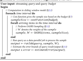
Algorithm 2 : StreamApprox’s algorithm overview User input: streamingqueryand querybudget
begin
//Computation in sliding window model (§2.2)
foreachtime intervaldo
//Cost function gives the sample size based on the budget (§7) sampleSize←costFunction(budget);
forallarriving items in the time intervaldo
//Perform OASRS Sampling (§3.2)
//Wdenotes the weights of thesample
sample,W ←OASRS(items,sampleSize); end
//Run query as a data-parallel job to process the sample output←runJob(query,sample,W);
//Estimate the error bounds of query result/output (§3.3) output±er ror←estimateError(output); end
end
across time intervals to adapt to user’s requirements for the budget.
3.2 Online Adaptive Stratified Reservoir Sampling To realize the real-time stream analytics, we propose a novel sam-pling technique called Online Adaptive Stratified Reservoir Sam-pling (OASRS). It achieves both stratified and reservoir samSam-plings without their drawbacks. Specifically, OASRS does not overlook any sub-streams regardless of their popularity, does not need to know the statistics of sub-streams before the sampling process, and runs efficiently in real time in a distributed manner.
The high-level idea of OASRS is simple, as described in Algo-rithm3. We stratify the input stream into sub-streams according to their sources. We assume data items from each sub-stream follow the same distribution and are mutually independent. (Here, a
stra-tumrefers to one sub-stream. If multiple sub-streams have the same distribution, they can be combined to form a stratum.) We then sample each sub-stream independently, and perform the reservoir sampling for each sub-stream individually. To do so, every time we encounter a new sub-streamSi, we determine its sample size Ni according to an adaptive cost function considering the speci-fied query budget (see §7). For each sub-streamSi, we perform the traditional reservoir sampling to select items at random from this sub-stream, and ensure that the total number of selected items from Si does not exceed its sample sizeNi. In addition, we maintain a counterCito measure the number of items received fromSiwithin the concerned time interval (see Figure2).
Applying reservoir sampling to each sub-streamSi ensures that we can randomly select at mostNi items from each sub-stream. The selected items from different sub-streams, however, shouldnot be treated equally. In particular, for a sub-streamSi, ifCi > Ni (i.e., the sub-streamSi has more thanNi items in total during the concerned time interval), then we randomly selectNi items from this sub-stream and each selected item representsCi/Nioriginal items on average; otherwise, ifCi ≤Ni, we select all the received Ciitems so that each selected item only represents itself. As a result, in order to statistically recreate the original items from the selected items, we assign a specific weightWi to the items selected from each sub-streamSi: Wi = Ci/Ni ifCi >Ni 1 ifCi ≤Ni (1) Sub-streams S1 S2 S3 Reservoir sampling Reservoir size (N = 3) Weights W1 = 6/3 (C1 = 6) W2 = 4/3 (C2 = 4) W3 = 1 (C3 = 2)
Figure 2.OASRS with the reservoirs of size three.
We supportapproximate linear querieswhich return an approxi-mate weighted sum of all items received from all sub-streams. One example of linear queries is to compute the sum of all received items. Suppose there are in totalX sub-streams{Si}X
i=1, and from each
sub-streamSiwe randomly select at mostNiitems. Specifically, we selectYi items{Ii,j}Yi
j=1from each sub-streamSi, whereYi ≤Ni.
In addition, each sub-stream associates with a weightWigenerated according to expression1. Then, the approximate sumSU Mi of all items received from each sub-streamSican be estimated as:
SU Mi =(
Yi
X
j=1
Ii,j)×Wi (2)
As a result, the approximate total sum of all items received from all sub-streams is:
SU M=
X
X
i=1
SU Mi (3)
A simple extension also enables us to compute the approximate mean value of all received items:
MEAN = SU M
PX
i=1Ci
(4)
Here,Ci denotes a counter measuring the number of items re-ceived from each sub-streamSi. Using a similar technique, our OASRS sampling algorithm supports any types of approximate lin-ear queries. This type of queries covers a range of common aggrega-tion queries including, for instance, sum, average, count, histogram, etc. Though linear queries are simple, they can be extended to sup-port a large range of statistical learning algorithms [11,12]. It is also worth mentioning that, OASRS not only works for a concerned time interval (e.g., a sliding time window), but also works with unbounded data streams.
To summarize, our proposed sampling algorithm combines the benefits of stratified and reservoir samplings via performing the reservoir sampling for each sub-stream (i.e., stratum) individu-ally. In addition, our algorithm is an online algorithm since it can perform the “on-the-fly” sampling on the input stream without knowing all data items in a window from its beginning [3].
Distributed execution.OASRS can run in a distributed fashion naturally as it does not require synchronization. One straightfor-ward approach is to make each sub-streamSi be handled by a set ofwworker nodes. Each worker node samples an equal portion of items from this sub-stream and generates a local reservoir of size no larger thanNi/w. In addition, each worker node maintains a local counter to measure the number of its received items within a concerned time interval for weight calculation. The rest of the design remains the same.
Algorithm 3 : Online adaptive stratified reservoir sampling
OASRS(items, sampleSize)
begin
sample← ∅;//Set of items sampled within the time interval S← ∅;//Set of sub-streams seen so far within the time interval W← ∅;//Set of weights of sub-streams within the time interval Update(S);//Update the set of sub-streams
//Determine the sample size for each sub-stream N←getSampleSize(sampleSize, S); forallSiinSdo
Ci←0;//Initial counter to measure #items in each sub-stream
forallarriving items in each time intervaldo
Update(Ci);//Update the counter
samplei←RS(items,Ni);//Reservoir sampling sample.add(samplei);//Update the global sample //Compute the weight ofsampleiaccording to Equation1
ifCi >Nithen Wi←CNii; end else Wi←1; end
W.add(Wi);//Update the set of weights
end end
returnsample,W end
3.3 Error Estimation
We described how we apply OASRS to randomly sample the input data stream to generate the approximate results for linear queries. We now describe a method to estimate the accuracy of our approxi-mate results via rigorous error bounds.
Similar to §3.2, suppose the input data stream containsX sub-streams{Si}X
i=1
. We compute the approximate sum of all items received from all sub-streams by randomly sampling onlyYi items from each sub-streamSi. As each sub-stream is sampled indepen-dently, the variance of the approximate sum is:
V ar(SU M)=
X
X
i=1
V ar(SU Mi) (5)
Further, as items are randomly selected for a sample within each sub-stream, according to the random sampling theory [40], the variance of the approximate sum can be estimated as:
M V ar(SU M)= X X i=1 Ci×(Ci−Yi)×s 2 i Yi (6)
Here,Ci denotes the total number of items from the sub-stream Si, andsi denotes the standard deviation of the sub-streamSi’s sampled items: s2 i = 1 Yi−1 × Yi X j=1 (Ii,j−I¯ i)2 , where ¯Ii = 1 Yi × Yi X j=1 Ii,j (7)
Next, we show how we can also estimate the variance of the approximate mean value of all items received from all theX sub-streams. According to equation4, this approximate mean value can
be computed as: MEAN=PSU MX i=1Ci = PX i=1(Ci ×MEANi) PX i=1Ci = X X i=1 (ωi×MEANi) (8) Here,ωi = Ci PX i=1Ci
. Then, as each sub-stream is sampled
in-dependently, according to the random sampling theory [40], the variance of the approximate mean value can be estimated as:
M V ar(MEAN)= X X i=1 V ar(ωi×MEANi) = X X i=1 ω2 i ×V ar(MEANi) = X X i=1 ω2 i × s2 i Yi × Ci−Yi Ci (9)
Above, we have shown how to estimate the variances of the approximate sum and the approximate mean of the input data stream. Similarly, by applying the random sampling theory, we can estimate the variance of the approximate results of any linear queries.
Error bound.According to the “68-95-99.7” rule [45], our approx-imate result falls within one, two, and three standard deviations away from the true result with probabilities of 68%, 95%, and 99.7%, respectively, where the standard deviation is the square root of the variance as computed above. This error estimation is critical because it gives us a quantitative understanding of the accuracy of our sampling technique.
4
Implementation
To showcase the effectiveness of our algorithm, we implemented StreamApprox based on two stream processing systems (§2.2):(i) Apache Spark Streaming [22], and(ii)Apache Flink [20].
Furthermore, we also built an improved baseline (in addition to the native execution) for Apache Spark, which provides sampling mechanisms for its machine learning library MLib [21]. In particular, werepurposedthe existing sampling modules available in Apache Spark (primarily used for machine learning) to build an approximate computing system for stream analytics. To have a fair comparison, we evaluated our Spark-based StreamApprox with two baselines: the Spark native execution and the improved Spark sampling based approximate computing system. Meanwhile, Apache Flink does not support sampling operations for stream analytics, therefore we compare our Flink-based StreamApprox with only the Flink native execution.
We next present the necessary background on Spark Streaming (and its existing sampling mechanisms) and Flink (§4.1). Thereafter, we provide the implementation details of our prototypes (§4.2). 4.1 Background
4.1.1 Apache Spark Streaming
Apache Spark Streaming splits the input data stream into micro-batches, and for each micro-batch a distributed data-parallel job (Spark job) is launched to process the micro-batch. Spark Streaming makes use of RDD-based sampling functions supported by Apache
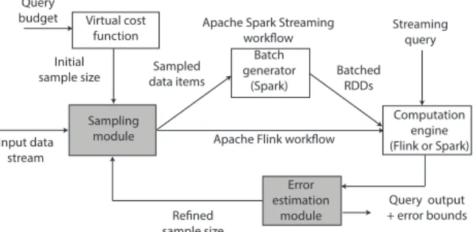
Batched RDDs Batch generator (Spark) Query output + error bounds Input data stream Sampled data items Computation engine (Flink or Spark) Query budget Refined sample size Virtual cost function Initial sample size Error estimation module Streaming query Sampling
module Apache Flink workflow Apache Spark Streaming
workflow
Figure 3.Architecture of StreamApprox prototypes (shaded boxes depict the implemented modules). We have implemented our system based on Apache Spark Streaming and Apache Flink.
Spark [46] to take a sample from each micro-batch. These functions can be classified into the following two categories: 1) Simple Ran-dom Sampling (SRS) usingsample, and 2) Stratified Sampling (STS) usingsampleByKeyandsampleByKeyExact.
Simple random sampling (SRS) is implemented using a random sort mechanism [33] which selects a sample of sizekfrom the input data items in two steps. In the first step, Spark assigns a random number in the range of [0,1] to each input data item to produce a value pair. Thereafter, in the next step, Spark sorts all key-value pairs based on their assigned random numbers, and selects kdata items with the smallest assigned random numbers. Since sorting “Big Data” is expensive, the second step quickly becomes a bottleneck in this sampling algorithm. To mitigate this bottleneck, Spark reduces the number of items before sorting by setting two thresholds,pandq, for the assigned random numbers. In particular, Spark discards the data items with the assigned random numbers larger thanq, and directly selects data items with the assigned numbers smaller thanp. For stratified sampling (STS), Spark first clusters the input data items based on a given criterion (e.g., data sources) to create strata usinggroupBy(strata). Thereafter, it applies the aforementioned SRS to data items in each stratum.
4.1.2 Apache Flink
In contrast to the batched stream processing, Apache Flink adopts a pipelined architecture: whenever an operator in the DAG dataflow emits an item, this item isimmediatelyforwarded to the next opera-tor without waiting for a whole data batch. This mechanism makes Apache Flink a true stream processing engine. In addition, Flink considers batches as a special case of streaming. Unfortunately, the vanilla Flink does not provide any operations to take a sample of the input data stream. In this work, we provide Flink with an oper-ator to sample input data streams by implementing our proposed sampling algorithm (see §3.2).
4.2 StreamApprox Implementation Details
We next describe the implementation of StreamApprox. Figure3 illustrates the architecture of our prototypes, where the shaded boxes depict the implemented modules. We showcase workflows for Apache Spark Streaming and Apache Flink in the same figure.
4.2.1 Spark-based StreamApprox
In the Spark-based implementation, the input data items are sam-pled “on-the-fly” using our sampling modulebeforeitems are trans-formed into RDDs. The sampling parameters are determined based on the query budget using a virtual cost function. In particular, a user can specify the query budget in the form of desired la-tency/throughput, available computational resources, or acceptable accuracy loss. As noted in the design assumptions (§2.3), we have not implemented the virtual cost function since it is beyond the scope of this paper (see §7for possible ways to implement such a cost function). Based on the query budget, the virtual cost function determines a sample size, which is then fed to the sampling module. Thereafter, the sampled input stream is transformed into RDDs, where the data items are split into batches at a pre-defined regular batch interval. Next, the batches are processed as usual using the Spark engine to produce the query output. Since the computed output is an approximate query result, we make use of our error estimation module to give rigorous error bounds. In cases where the error bound is larger than the specified target, an adaptive feedback mechanism is activated to increase the sample size in the sampling module. This way, we achieve higher accuracy in the subsequent epochs.
I: Sampling module.The sampling module implements the algo-rithm described in §3.2to select samples from the input data stream in an online adaptive fashion. We modified the Apache Kafka con-nector of Spark to support our sampling algorithm. In particular, we created a new classApproxKafkaRDDto handle the input data items from Kafka, which takes required samples to define an RDD for the data items before calling thecomputefunction.
II: Error estimation module.The error estimation module com-putes the error bounds of the approximate query result. The module also activates a feedback mechanism to re-tune the sample size in the sampling module to achieve the specified accuracy target. We made use of the Apache Common Math library [32] to implement the error estimation mechanism as described in §3.3.
4.2.2 Flink-based StreamApprox
Compared to the Spark-based implementation, a Flink-based StreamAp-prox is straightforward to implement since Flink supports online stream processing natively.
I: Sampling module.We created a sampling operator by imple-menting the algorithm described in §3.2. This operator samples input data items on-the-fly and in an adaptive manner. The sam-pling parameters are identified based on the query budget as in Spark-based StreamApprox.
II: Error estimation module.We reused the error estimation module implemented in the Spark-based StreamApprox.
5
Evaluation
In this section, we present the evaluation results of our implemen-tation. In the next section, we report our experiences on deploying StreamApprox for real-world case studies (§6).
5.1 Experimental Setup
Synthetic data stream.To understand the effectiveness of our proposed OASRS sampling algorithm, we first evaluated StreamAp-prox using a synthetic input data stream with Gaussian distribution
0 1 2 3 4 5 6 7 8 10 20 40 60 80 Native Throughput ( M) #items/s Sampling fraction (%) (a) Throughput vs Sampling fraction
Flink-based StreamApprox Spark-based StreamApprox Spark-based SRS Spark-based STS Native Flink Native Spark 0 1 2 3 10 20 40 60 80 90 Accuracy los s (%) Sampling fraction (%)
(b) Accuracy loss vs Sampling fraction
Flink-based StreamApprox Spark-based StreamApprox Spark-based SRS Spark-based STS 0 1 2 3 4 5 250 500 1000 Throughput ( M) #items/s Batch interval (ms) (c) Throughput vs Batch intervals
Spark-based StreamApprox Spark-based SRS Spark-based STS
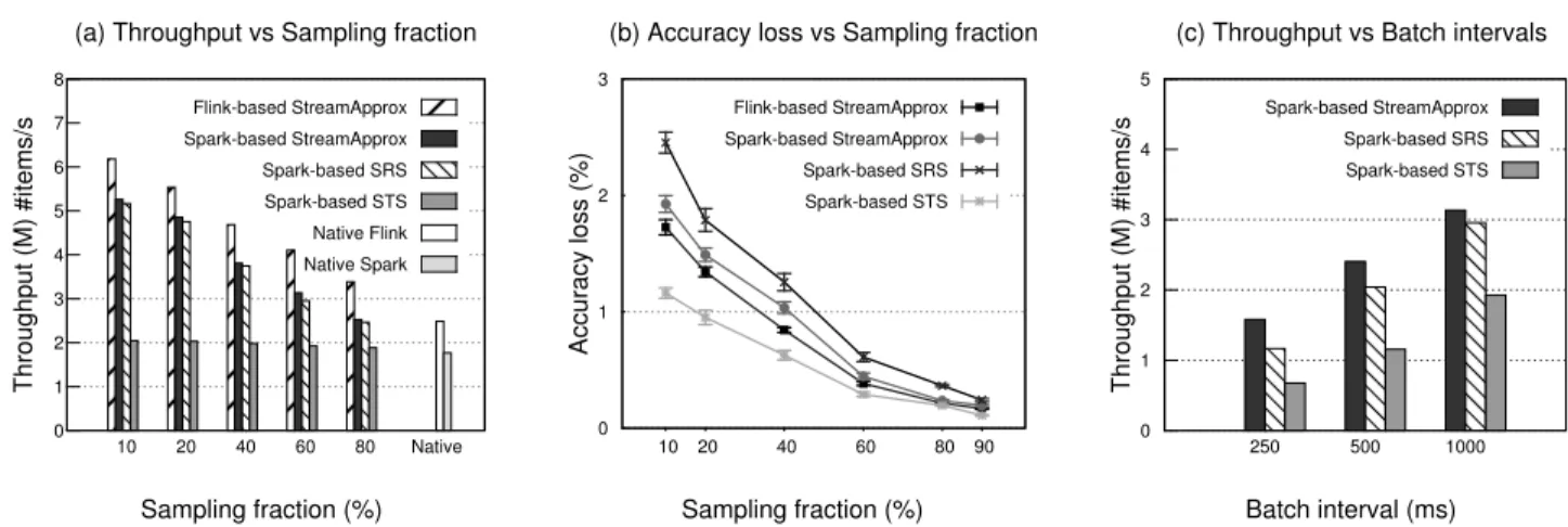
Figure 4.Comparison b/w StreamApprox, Spark-based SRS, Spark-based STS, as well as the native Spark and Flink systems. (a) Throughput with varying sampling fractions. (b) Accuracy loss with varying sampling fractions. (c) Throughput with different batch intervals.
and Poisson distribution. For the Gaussian distribution, unless spec-ified otherwise, we used three input sub-streamsA,B, andCwith their data items following Gaussian distributions with parameters (µ =10, σ =5), (µ =1000, σ =50), and (µ =10000, σ =500), respectively. For the Poisson distribution, unless specified other-wise, we used three input sub-streamsA,B, andCwith their data items following Poisson distributions with parameters (λ =10), (λ=1000), and (λ=100000000), respectively.
Methodology for comparison with Apache Spark.For a fair comparison with the sampling algorithms available in Apache Spark, we also built an Apache Spark-based approximate comput-ing system for stream analytics (as described in§4). In particular, we used two sampling algorithms available in Spark, namely, Sim-ple Random Sampling (SRS) viasample, and Stratified Sampling (STS) viasampleByKeyandsampleByKeyExact. We applied these sampling operators to each small batch (i.e., RDD) in the input data stream to generate samples. Note that Apache Flink does not support sampling natively.
Evaluation questions.Our evaluation analyzes the performance of StreamApprox, and compares it with the Spark-based approxi-mate computing system across the following dimensions: (a) vary-ing sample sizes in§5.2, (b) varying batch intervals in§5.3, (c) varying arrival rates for sub-streams in§5.4, (d) varying window sizes in§5.5, (e) scalability in§5.6, and (f ) skew in the input data stream in§5.7.
5.2 Varying Sample Sizes
Throughput.We first measure the throughput of StreamApprox w.r.t. the Spark- and Flink-based systems with varying sample sizes (sampling fractions). To measure the throughput of the evaluated systems, we increase the arrival rate of the input stream until these systems are saturated.
Figure4(a) first shows the throughput comparison of StreamAp-prox and the two sampling algorithms in Spark. Spark-based strat-ified sampling (STS) scales poorly because of its synchronization among Spark workers and the expensive sorting during its sampling process (as detailed in§4.1). Spark-based StreamApprox achieves a throughput of 1.68×and 2.60×higher than Spark-based STS with
sampling fractions of 60% and 10%, respectively. In addition, Spark-based simple random sampling (SRS) scales better than STS and has a similar throughput as in StreamApprox, but SRS loses the capability of considering each sub-stream fairly.
Meanwhile, Flink-based StreamApprox achieves a throughput of 2.13×and 3×higher than Spark-based STS with sampling frac-tions of 60% and 10%, respectively. This is mainly due to the fact that Flink is a truly pipelined stream processing engine. Moreover, Flink-based StreamApprox achieves a throughput of 1.3× com-pared to Spark-based StreamApprox and Spark-based SRS with the sampling fraction of 60%.
We also compare StreamApprox with native Spark and Flink systems, i.e., without any sampling. With the sampling fraction of 60%, the throughput of Spark-based StreamApprox is 1.8×higher than the native Spark execution, whereas the throughput of Flink-based StreamApprox is 1.65×higher than the native Flink. Accuracy.Next, we compare the accuracy of our proposed OASRS sampling with that of the two sampling mechanisms with the vary-ing samplvary-ing fractions. Figure4(b) first shows that StreamAp-prox systems and Spark-based STS achieve a higher accuracy than Spark-based SRS. For instance, with the sampling fraction of 60%, Flink-based StreamApprox, Spark-based StreamApprox, and Spark-based STS achieve the accuracy loss of 0.38%, 0.44%, and 0.29%, respectively, which are higher than Spark-based SRS that only achieves the accuracy loss of 0.61%. This higher accuracy is due to the fact that both StreamApprox and Spark-based STS integrate stratified sampling which ensures that data items from each sub-stream are selected fairly. In addition, Spark-based STS achieves even higher accuracy than StreamApprox, but recall that Spark-based STS needs to maintain a sample size of each sub-stream proportional to the size of the sub-stream (see §4.1). This leads to a much lower throughput than StreamApprox which only maintains a sample of a fixed size for each sub-stream.
5.3 Varying Batch Intervals
Spark-based systems adopt the batched stream processing model. Next, we evaluate the impact of varying batch intervals on the performance of Spark-based StreamApprox, Spark-based SRS, and Spark-based STS system. We keep the sampling fraction as 60%
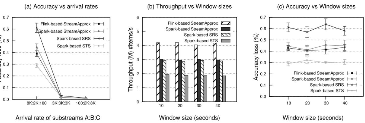
0.0 0.1 0.2 0.3 0.4 0.5 0.6 0.7 8K:2K:100 3K:3K:3K 100:2K:8K Accuracy los s (%)
Arrival rate of substreams A:B:C (a) Accuracy vs arrival rates
Flink-based StreamApprox Spark-based StreamApprox Spark-based SRS Spark-based STS 0 1 2 3 4 5 6 10 20 30 40 Throughput ( M) #items/s
Window size (seconds) (b) Throughput vs Window sizes
Flink-based StreamApprox Spark-based StreamApprox Spark-based SRS Spark-based STS 0.0 0.1 0.2 0.3 0.4 0.5 0.6 0.7 10 20 30 40 Accuracy los s (%)
Window size (seconds) (c) Accuracy vs Window sizes
Flink-based StreamApprox Spark-based StreamApprox Spark-based SRS Spark-based STS
Figure 5.Comparison between StreamApprox, Spark-based SRS, and Spark-based STS. (a) Accuracy loss with varying arrival rates. (b) Throughput with varying window sizes. (c) Accuracy loss with varying window sizes.
and measure the throughput of each system with different batch intervals.
Figure4(c) shows that, as the batch interval becomes smaller, the throughput ratio between Spark-based systems gets bigger. For instance, with the 1000ms batch interval, the throughput of Spark-based StreamApprox is 1.07×and 1.63×higher than the throughput of Spark-based SRS and STS, respectively; with the 250ms batch interval, the throughput of StreamApprox is 1.36× and 2.33×higher than the throughput of Spark-based SRS and STS, respectively. This is because Spark-based StreamApprox samples the data items without synchronization before forming RDDs and significantly reduces costs in scheduling and processing the RDDs, especially when the batch interval is small.
5.4 Varying Arrival Rates for Sub-Streams
In the following experiment, we evaluate the impact of varying rates of sub-streams. We used an input data stream with Gaussian distributions as described in§5.1. We maintain the sampling frac-tion of 60% and measure the accuracy loss of the four Spark- and Flink-based systems with different settings of arrival rates.
Figure5(a) shows the accuracy loss of these four systems. The accuracy loss decreases proportionally to the increase of the arrival rate of the sub-streamCwhich carries the most significant data items compared to other sub-streams. When the arrival rate of the sub-streamCis set to 100 items/second, Spark-based SRS system achieves the worst accuracy since it may overlook sub-streamC which contributes only a few data items but has significant values. On the other hand, when the arrival rate of sub-streamCis set to 8000 items/second, the four systems achieve almost the same accuracy. This is mainly because all four systems do not overlook sub-streamCwhich contains items with the most significant values. 5.5 Varying Window Sizes
Next, we evaluate the impact of varying window sizes on the throughput and accuracy of the four systems. We used the same input as described in§5.4with its three sub-streams’ arrival rates being 8000, 2000, and 100 items per second. Figure5(b) and Figure5 (c) show that the window sizes of the computation do not affect the throughput and accuracy of these systems significantly. This
is because the sampling operations are performed at every batch interval in the Spark-based systems and at every slide window interval in the Flink-based StreamApprox.
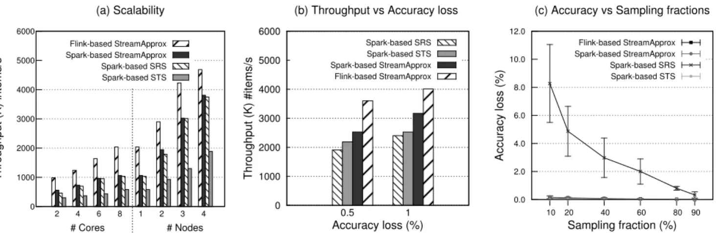
5.6 Scalability
To evaluate the scalability of StreamApprox, we keep the sampling fraction as 40% and measure the throughput of StreamApprox and the Spark-based systems with different numbers of CP U cores (scale-up) and different numbers of nodes (scale-out).
Figure6(a) shows unsurprisingly that StreamApprox and Spark-based SRS scale better than Spark-Spark-based STS. For instance, with one node (8 cores), the throughput of Spark-based StreamApprox and Spark-based SRS is roughly 1.8×higher than that of Spark-based STS. With three nodes, based StreamApprox and Spark-based SRS achieve a speedup of 2.3×over Spark-based STS. In addition, Flink-based StreamApprox achieves a throughput even 1.9×and 1.4×higher compared to Spark-based StreamApprox with one node and three nodes, respectively.
5.7 Skew in the Data Stream
Lastly, we study the effect of the non-uniformity in sub-stream sizes. In this experiment, we construct an input data stream where one of its sub-streams dominates the other sub-streams. In particular, we evaluated the skew in the input stream using two data distributions:
(i)Gaussian distribution and(ii)Poisson distribution.
I: Gaussian distribution.First, we generated an input data stream consisting of three sub-streamsA,B, andC with the Gaussian distribution of parameters (µ = 100, σ = 10), (µ = 1000, σ = 100), and (µ =10000, σ =1000), respectively. The sub-streamA comprises 80% of the data items in the entire data stream, whereas the sub-streamsBandCcomprise only 19% and 1% of data items, respectively. We set the sliding window size tow=10 seconds, and each sliding step toδ =5 seconds.
Figure7(a), (b), and (c) present the mean values of the received data items produced by the three Spark-based systems every 5 seconds during a 10-minute observation. As expected, Spark-based STS and StreamApprox provide more accurate results than Spark-based SRS because Spark-Spark-based STS and StreamApprox ensure
0 1000 2000 3000 4000 5000 6000 2 4 6 8 1 2 3 4 Throughput ( K) #items/s (a) Scalability # Cores # Nodes Flink-based StreamApprox Spark-based StreamApprox Spark-based SRS Spark-based STS 0 1000 2000 3000 4000 5000 6000 0.5 1 Throughput ( K) #items/s Accuracy loss (%) (b) Throughput vs Accuracy loss
Spark-based SRS Spark-based STS Spark-based StreamApprox Flink-based StreamApprox 0.0 2.0 4.0 6.0 8.0 10.0 12.0 10 20 40 60 80 90 Accuracy los s (%) Sampling fraction (%) (c) Accuracy vs Sampling fractions
Flink-based StreamApprox Spark-based StreamApprox Spark-based SRS Spark-based STS
Figure 6.Comparison between StreamApprox, Spark-based SRS, and Spark-based STS. (a) Throughput with different numbers of CP U cores and nodes. (b) Throughput with accuracy loss. (c) Accuracy loss with varying sampling fractions.
300 350 400 450 500 0 20 40 60 80 100 120 Mean Time (5s)
(a) Simple Random Sampling (SRS)
Ground truth(w/o sampling) Spark-based SRS 300 350 400 450 500 0 20 40 60 80 100 120 Mean Time (5s) (b) Stratified Sampling (STS)
Ground truth(w/o sampling) Spark-based STS 300 350 400 450 500 0 20 40 60 80 100 120 Mean Time (5s) (c) StreamApprox
Ground truth(w/o sampling) StreamApprox
Figure 7.The mean values of the received data items produced by different sampling techniques every 5 seconds during a 10-minute observation. The sliding window size is 10 seconds, and each sliding step is 5 seconds.
that the data items from the minority (i.e., sub-streamC) are fairly selected in the samples.
In addition, we keep the accuracy loss across all four systems the same and then measure their respective throughputs. Figure6 (b) shows that, with the same accuracy loss of 1%, the throughput of Spark-based STS is 1.05×higher than Spark-based SRS, whereas Spark-based StreamApprox achieves a throughput 1.25×higher than Spark-based STS. In addition, Flink-based StreamApprox achieves the highest throughput which is 1.68×, 1.6×, and 1.26× higher than Spark-based SRS, Spark-based STS, and Spark-based StreamApprox, respectively.
II: Poisson distribution.In the next experiment, we generated an input data stream with the Poisson distribution as described in§5.1. The sub-streamAaccounts for 80% of the entire data stream items, while the sub-streamBaccounts for 19.99% and the sub-streamC comprises only 0.01% of the data stream items, respectively. Figure6 (c) shows that StreamApprox systems and Spark-based STS outper-form Spark-based SRS in terms of accuracy. The reason for this is
StreamApprox systems and Spark-based STS do not overlook sub-streamCwhich has items with significant values. Furthermore, this result strongly demonstrates the superiority of our proposed sam-pling algorithm OASRS over simple random samsam-pling in processing long-tail data which is very common in practice.
6
Case Studies
In this section, we report our experiences and results with the following two real-world case studies: (a) network traffic analytics (§6.2) and (b) New York taxi ride analytics (§6.3).
6.1 Experimental Setup
Cluster setup.We performed experiments using a cluster of 17 nodes. Each node in the cluster has 2 Intel Xeon E5405 CP Us (quad core), 8GB of RAM, and a SATA-2 hard disk, running Ubuntu 14.04.5 LTS. We deployed our StreamApprox prototype on 5 nodes (1 driver node and 4 worker nodes), the traffic replay tool on 5 nodes, the Apache Kafka-based stream aggregator on 4 nodes, and the Apache Zookeeper [23] on the remaining 3 nodes.
0 500 1000 1500 2000 2500 3000 10 20 40 60 80 Native Throughput (K) #items/s Sampling fraction (%) (a) Throughput vs Sampling fraction
Flink-based StreamApprox Spark-based StreamApprox Spark-based SRS Spark-based STS Native Flink Native Spark 0 1 2 3 10 20 40 60 80 90 Accuracy loss (%) Sampling fraction (%) (b) Accuracy loss vs Sampling fraction
Flink-based StreamApprox Spark-based StreamApprox Spark-based SRS Spark-based STS 0 500 1000 1500 2000 2500 3000 1 2 Throughput (K) #items/s Accuracy loss (%) (c) Throughput vs Accuracy loss
Flink-based StreamApprox Spark-based StreamApprox Spark-based SRS Spark-based STS
Figure 8.Network traffic analytics case-study: (a) Throughput with varying sampling fractions. (b) Accuracy loss with varying sampling fractions. (c) Throughput with different accuracy losses.
Measurements.We evaluated StreamApprox using the follow-ing key metrics: (a) throughput: measured as the number of data items processed per second; (b) latency: measured as the total time required for processing the respective dataset; and lastly, (c) accu-racy loss: measured as|approx−exact|/exactwhereapproxand exactdenote the results from StreamApprox and a native system without sampling, respectively.
Methodology.We built a tool to efficiently replay the case-study dataset as the input data stream. In particular, for the throughput measurement, we tuned the replay tool to first feed 2000 mes-sages/second and continued to increase the throughput until the system was saturated. Here, each message contained 200 data items. For comparison, we report results from StreamApprox, Spark-based SRS, Spark-Spark-based STS systems, as well as the native Spark and Flink systems. For all experiments, we report measurements based on the average over 10 runs. Lastly, the sliding window size was set to 10 seconds, and each sliding step was set to 5 seconds.
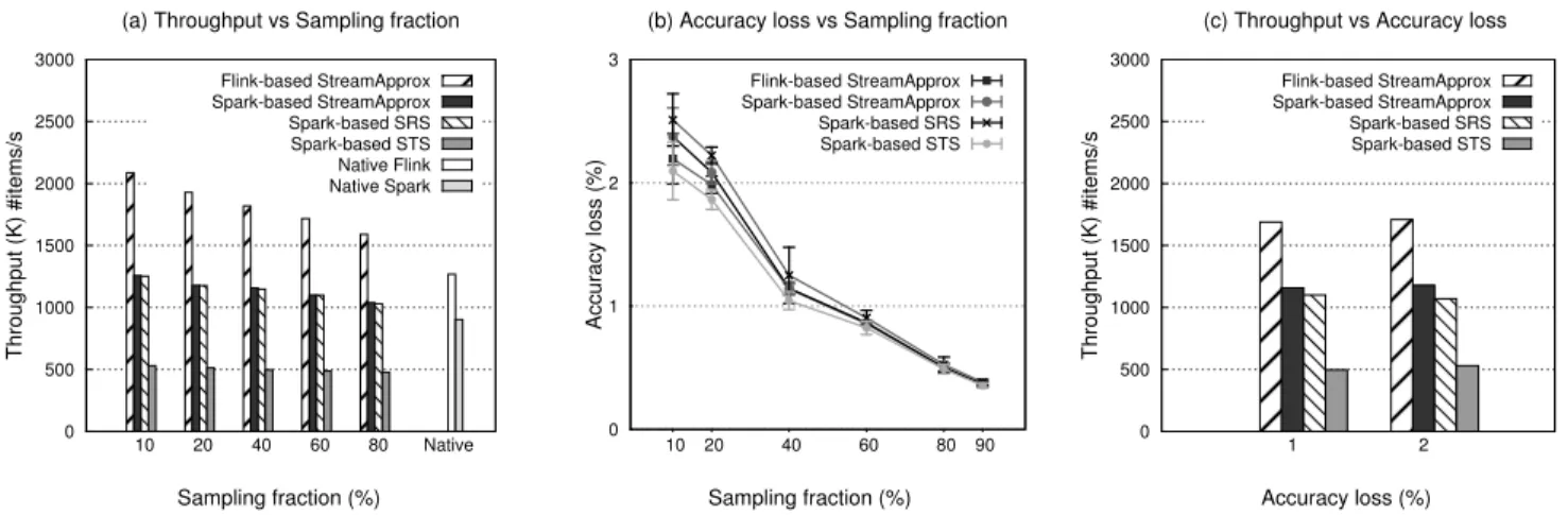
6.2 Network Traffic Analytics
In the first case study, we deployed StreamApprox for a real-time network traffic monitoring application to measure the TCP, UDP, and ICMP network traffic over time.
Dataset.We used the publicly-available 670GB network traces from CAIDA [13]. These were recorded on the high-speed Internet backbone links in Chicago in 2015. We converted the raw network traces into the NetFlow format [15], and then removed unused fields (such as source and destination ports, duration, etc.) in each NetFlow record to build a dataset for our experiments. The dataset contains 115,472,322 TCP flows, 67,098,852 UDP flows, and 2,801,002 ICMP flows. Each stream data item is a flow record in the dataset.
Query.We deployed the evaluated systems to measure the total sizes of TCP, UDP, and ICMP network traffic in each sliding window.
Results.Figure8(a) presents the throughput comparison between StreamApprox, Spark-based SRS, Spark-based STS systems, as well as the native Spark and Flink systems. The result shows that Spark-based StreamApprox achieves more than 2×throughput
than Spark-based STS, and achieves a similar throughput com-pared with Spark-based SRS (which loses the capability of consid-ering each sub-stream fairly). In addition, due to Flink’s pipelined stream processing model, Flink-based StreamApprox achieves a throughput even 1.6×higher than Spark-based StreamApprox and Spark-based SRS. We also compare StreamApprox with the native Spark and Flink systems. With the sampling fraction of 60%, the throughput of Spark-based StreamApprox is 1.3×higher than the native Spark execution, whereas the throughput of Flink-based StreamApprox is 1.35×higher than the native Flink execution. Surprisingly, the throughput of the native Spark execution is even higher than the throughput of Spark-based STS. This is because Spark-based STS requires the expensive extra steps (see§4.1).
Figure8(b) shows the accuracy loss with different sampling fractions. As the sampling fraction increases, the accuracy loss of StreamApprox, Spark-based SRS, and Spark-based STS decreases (i.e., accuracy improves), but not linearly. StreamApprox systems produce more accurate results than Spark-based SRS but less ac-curate results than Spark-based STS. Note however that, although both StreamApprox systems and Spark-based STS integrate strati-fied sampling to ensure that every sub-stream is considered fairly, StreamApprox systems are much more resource-friendly than Spark-based STS. This is because Spark-based STS requires per-forming the expensiveдroupByKeyoperation as well as synchro-nization among workers to take samples from the input data stream, whereas StreamApprox performs the sampling operation with a configurable sample size for sub-streams requiring no synchroniza-tion between workers.
In addition, to show the benefit of StreamApprox, we fixed the same accuracy loss for all four systems and then compared their respective throughputs. Figure8(c) shows that, with the accuracy loss of 1%, the throughput of Spark-based StreamApprox is 2.36× higher than Spark-based STS, and 1.05×higher than Spark-based SRS. Flink-based StreamApprox achieves a throughput even 1.46× higher than Spark-based StreamApprox.
Finally, to make a comparison in terms of latency between these systems, we created sampling functionsampleOASRS()for Spark RDD by implementing our proposed sampling algorithm OASRS,
0 500 1000 1500 2000 2500 3000 3500 4000 10 20 40 60 80 Native Throughput (K) #items/s Sampling fraction (%) (a) Throughput vs Sampling fraction
Flink-based StreamApprox Spark-based StreamApprox Spark-based SRS Spark-based STS Native Flink Native Spark 0 0.2 0.4 0.6 0.8 10 20 40 60 80 90 Accuracy loss (%) Sampling fraction (%) (b) Accuracy loss vs Sampling fraction
Flink-based StreamApprox Spark-based StreamApprox Spark-based SRS Spark-based STS 0 500 1000 1500 2000 2500 3000 3500 4000 0.1 0.4 Throughput (K) #items/s Accuracy loss (%) (c) Throughput vs Accuracy loss
Flink-based StreamApprox Spark-based StreamApprox Spark-based SRS Spark-based STS
Figure 9.New York taxi ride analytics case-study: (a) Throughput with varying sampling fractions. (b) Accuracy loss with varying sampling fractions. (c) Throughput with different accuracy losses.
0 20 40 60 80 100 120 140 160 180 STS SRS Stream Approx Latency (second s) Network traffic NYC taxi
Figure 10. The latency comparison between StreamApprox, Spark-based SRS, and Spark-based STS with the real-world datasets. The sampling fraction is set to 60%.
and then measured the latency in processing the network traf-fic dataset. Figure10indicates that the latency of Spark-based StreamApprox is 1.39×and 1.69×lower than Spark-based SRS and Spark-based STS in processing the network traffic dataset.
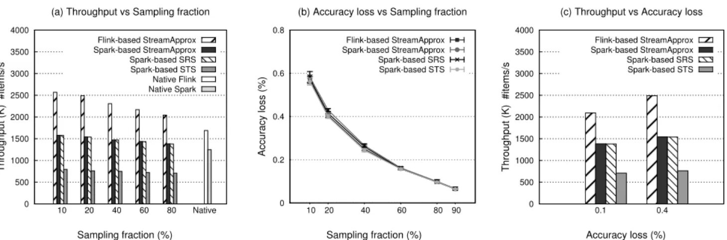
6.3 New York Taxi Ride Analytics
In the second case study, we evaluated StreamApprox with a taxi ride dataset to measure the average distance of trips starting from different boroughs in New York City.
Dataset.We used theNYC Taxi Ridedataset from the DEBS 2015 Grand Challenge [28]. The dataset consists of the itinerary infor-mation of all rides across 10,000 taxies in New York City in 2013. In addition, we mapped the start coordinates of each trip in the dataset into one of the six boroughs in New York.
Query.We deployed StreamApprox, based SRS, Spark-based STS systems, as well as the native Spark and Flink systems to measure the average distance of the trips starting from various boroughs in each sliding window.
Results.Figure9(a) shows that Spark-based StreamApprox achieves a similar throughput compared with Spark-based SRS (which, how-ever, does not consider each sub-stream fairly), and a roughly 2× higher throughput than Spark-based STS. In addition, due to Flink’s pipelined streaming model, Flink-based StreamApprox achieves a
1.5×higher throughput compared to Spark-based StreamApprox and Spark-based SRS. We again compared StreamApprox with the native Spark and Flink systems. With the sampling fraction of 60%, the throughput of Spark-based StreamApprox is 1.2×higher than the throughput of the native Spark execution, whereas the throughput of Flink-based StreamApprox is 1.28×higher than the throughput of the native Flink execution. Similar to the result in the first case study, the throughput of the native Spark execution is higher than the throughput of Spark-based STS.
Figure9 (b) depicts the accuracy loss of these systems with different sampling fractions. The results show that they all achieve a very similar accuracy in this case study. In addition, we also fixed the same accuracy loss of 1% for all four systems to measure their respective throughputs. Figure9(c) shows that Flink-based StreamApprox achieves the best throughput which is 1.6×higher than Spark-based StreamApprox and Spark-based SRS, and 3× higher than Spark-based STS. Figure10further indicates that Spark-based StreamApprox provides the 1.52×and 2.18×lower latency than Spark-based SRS and Spark-based STS.
7
Discussion
The design of StreamApprox is based on the assumptions men-tioned in§2.3. In this section, we discuss some approaches that could be used to meet our assumptions.
I: Virtual cost function.We currently assume that there exists a virtual cost function to translate a user-specified query budget into the sample size. The query budget could be specified as either available computing resources, desired accuracy or latency.
For instance, with an accuracy budget, we can define the sample size for each sub-stream based on a desired width of the confidence interval using Equation9and the “68-95-99.7” rule. With a desired latency budget, users can specify it by defining the window time interval or the slide interval for the computations over the input data stream. It becomes a bit more challenging to specify a budget for resource utilization. Nevertheless, we discuss some existing techniques that could be used to implement such a cost function to achieve the desired resource target. In particular, we refer to the two existing techniques: (a) virtual data center [4], and (b) resource prediction model [44] for latency requirements.
Pulsar [4] proposes an abstraction of a virtual data center (VDC) to provide performance guarantees to tenants in the cloud. In partic-ular, Pulsar makes use of a virtual cost function to translate the cost of a request processing into the required computational resources using a multi-resource token algorithm. We could adapt the cost function for our purpose as follows: we consider a data item in the input stream as a request and the “amount of resources” required to process it as the cost in tokens. Also, the given resource budget is converted in the form of tokens, using the pre-advertised cost model per resource. This allows us to compute the sample size that can be processed within the given resource budget.
For any given latency requirement, we could employ a resource prediction model [42–44]. In particular, we could build the predic-tion model by analyzing the diurnal patterns in resource usage [14] to predict the future resource requirement for the given latency bud-get. This resource requirement can then be mapped to the desired sample size based on the same approach as described above.
II: Stratified sampling.In our design in§3, we currently assume that the input stream is already stratified based on the source of data items, i.e., the data items within each stratum follow the same distribution — it does not have to be a normal distribution. This assumption ensures that our error estimation mechanism still holds correct since we apply the Central Limit Theorem. For example, consider an IoT use-case which analyzes data streams from sen-sors to measure the temperature of a city. The data stream from each individual sensor follows the same distribution since it mea-sures the temperature at the same location in the city. Therefore, a straightforward way to stratify the input data streams is to consider each sensor’s data stream as a stratum (sub-stream). In more com-plex cases where we cannot classify strata based on the sources, we need a pre-processing step to stratify the input data stream. This stratification problem is orthogonal to our work, nevertheless for completeness, we discuss two proposals for the stratification of evolving streams: bootstrap [19] and semi-supervised learning [31].
Bootstrap [19] is a well-studied non-parametric sampling tech-nique in statistics for the estimation of distribution for a given population. In particular, the bootstrap technique randomly selects “bootstrap samples” with replacement to estimate the unknown parameters of a population, for instance, by averaging the boot-strap samples. We can employ a bootboot-strap-based estimator for the stratification of incoming sub-streams. Alternatively, we could also make use of a semi-supervised algorithm [31] to stratify a data stream. The advantage of this algorithm is that it can work with both labeled and unlabeled streams to train a classification model.
8
Related Work
Given the advantages of making a trade-off between accuracy and efficiency, approximate computing is applied to various do-mains [38]. Our work mainly builds on the advancements in the databases community.
Over the last two decades, the databases community has pro-posed various approximation techniques based on sampling [2,25], online aggregation [27], and sketches [16]. These techniques make different trade-offs w.r.t. the output quality, supported queries, and workload. However, the early work in approximate computing was mainly geared towards the centralized database architecture.
Recently, sampling-based approaches have been successfully adopted for distributed data analytics [1,26,29,36,39]. In particular,
BlinkDB [1] proposes an approximate distributed query processing engine that uses stratified sampling [2] to support ad-hoc queries with error and response time constraints. ApproxHadoop [26] uses multi-stage sampling [30] for approximate MapReduce job execu-tion. Both BlinkDB and ApproxHadoop show that it is possible to make a trade-off between the output accuracy and the performance gains (also the efficient resource utilization) by employing sampling-based approaches to compute over a subset of data items. However, these “big data” systems target batch processing and cannot provide required low-latency guarantees for stream analytics.
Like BlinkDB, Quickr [39] also supports complex ad-hoc queries in big-data clusters. Quickr deploys distributed sampling opera-tors to reduce execution costs of parallelized queries. In particular, Quickr first injects sampling operators into the query plan; there-after, it searches for an optimal query plan among sampled query plans to execute input queries. However, Quickr is also designed for static databases, and it does not account for stream analytics. IncApprox [29] is a data analytics system that combines two com-puting paradigms together, namely, approximate and incremental computations [9,10] for stream analytics. The system is based on an online “biased sampling” algorithm that uses self-adjusting computation [5,8] to produce incrementally updated approximate output. Lastly, PrivApprox [36] supports privacy-preserving data analytics using a combination of randomized response and approx-imate computation. By contrast, in StreamApprox, we designed an “online” sampling algorithm solely for approximate computing, while avoiding the limitations of existing sampling algorithms.
9
Conclusion
In this paper, we presented StreamApprox, a stream analytics system for approximate computing. StreamApprox allows users to make a systematic trade-off between the output accuracy and the computation efficiency. To achieve this goal, we designed an online stratified reservoir sampling algorithm which ensures the statistical quality of the sample selected from the input data stream. Our proposed sampling algorithm is generalizable to two promi-nent types of stream processing models: batched and pipelined stream processing models. To showcase the effectiveness of our proposed algorithm, we built StreamApprox based on Apache Spark Streaming and Apache Flink.
We evaluated the effectiveness of our system using a series of micro-benchmarks and real-world case studies. Our evaluation shows that, with varying sampling fractions of 80% to 10%, Spark-and Flink-based StreamApprox achieves a significantly higher throughput of 1.15×—3×compared to the native Spark Streaming and Flink executions, respectively. Furthermore, StreamApprox achieves a speedup of 1.1×—2.4×compared to a Spark-based sam-pling system for approximate computing, while maintaining the same level of accuracy for the query output. Finally, the source code of StreamApprox along with the experimental setup is publicly available:https://streamapprox.github.io/.
Acknowledgments.We thank anonymous reviewers and our shep-herd Jan S. Rellermeyer for their helpful comments. This work is supported by the resilience path within CFAED at TU Dresden, the European Unions Horizon 2020 research and innovation pro-gramme under grant agreements 645011 (SERECA), Amazon Web Services Education Grant, and Microsoft Azure Grant.