Topics in Data Stream Sampling and Insider Threat Detection

(1)

2016

Topics in Data Stream Sampling and Insider Threat

Detection

Yung-Yu Chung

Iowa State University

Follow this and additional works at:

https://lib.dr.iastate.edu/etd

Part of the

Computer Engineering Commons

This Dissertation is brought to you for free and open access by the Iowa State University Capstones, Theses and Dissertations at Iowa State University Digital Repository. It has been accepted for inclusion in Graduate Theses and Dissertations by an authorized administrator of Iowa State University Digital Repository. For more information, please contactdigirep@iastate.edu.

Recommended Citation

Chung, Yung-Yu, "Topics in Data Stream Sampling and Insider Threat Detection" (2016).Graduate Theses and Dissertations. 15282. https://lib.dr.iastate.edu/etd/15282

(2)

by

Yung-Yu Chung

A dissertation submitted to the graduate faculty in partial fulfillment of the requirements for the degree of

DOCTOR OF PHILOSOPHY

Major: Computer Engineering

Program of Study Committee: Srikanta Tirthapura, Major Professor

Suraj C Kothari Soma Chaudhuri

Yong Guan Pavankumar R Aduri

Iowa State University Ames, Iowa

2016

(3)

Dedication

I would like to dedicate this thesis to my parents, who support me on my way researching in this area, and encourage me achieving my goal. I would also like to dedicate this thesis to my wife, Yu-Ciao Li, whose love and dedication is my strength to keep working on my goal and to be better. Without her constantly encouragement and accompaniment, I wouldn’t be able to keep on my path. I would like to thank my friends either here in Ames or in the other nations.

(4)

TABLE OF CONTENTS

LIST OF TABLES . . . vi

LIST OF FIGURES . . . vii

ABSTRACT . . . xii

CHAPTER 1. INTRODUCTION . . . 1

1.1 Data Stream Sampling . . . 1

1.2 Insider Threat Detection . . . 4

CHAPTER 2. CONTRIBUTION . . . 6

2.1 Random Sampling from a Distributed Stream . . . 6

2.2 Distinct Random Sampling from a Distributed Stream . . . 8

2.3 Insider Threat Detection from Log Streams . . . 9

CHAPTER 3. LITERATURE REVIEW . . . 11

3.1 Random Sampling from a Distributed Stream . . . 11

3.2 Distinct Random Sampling from a Distributed Stream . . . 12

3.3 Insider Threat Detection from Log Streams . . . 13

PART I DATA STREAM SAMPLING 15 CHAPTER 4. DISTRIBUTED RANDOM SAMPLING ON A DATA STREAM 16 4.1 Model . . . 16

4.2 Algorithm . . . 17

4.3 Analysis of the Algorithm (Upper Bound) . . . 19

(5)

4.5 Analysis Under Skew . . . 29

4.6 Sampling With Replacement . . . 33

4.7 Experiments . . . 34

CHAPTER 5. DISTINCT RANDOM SAMPLING ON A DISTRIBUTED DATA STREAM . . . 43

5.1 Model . . . 43

5.2 Infinite Window . . . 44

5.2.1 Infinite Window: Analysis . . . 46

5.2.2 Sampling With Replacement . . . 50

5.3 Sliding Window . . . 52

5.3.1 Sliding Window Analysis . . . 57

5.3.2 Lower Bound . . . 59

5.4 Experiments . . . 60

5.4.1 Infinite Window . . . 61

5.4.2 Sliding Window . . . 69

PART II INSIDER THREAT DETECTION 74 CHAPTER 6. INSIDER THREAT DETECTION OVER LOG STREAMS . 75 6.1 Overview . . . 75

6.2 Detection Approach . . . 75

6.2.1 Session-based Anomaly Detection . . . 75

6.2.2 Scenario-based Anomaly Detection . . . 76

6.3 Session-based Anomaly Detection . . . 77

6.3.1 Architecture of Unsupervised Insider Threat Detection . . . 77

6.4 Scenario-based Anomaly Detection . . . 79

6.4.1 System Architecture . . . 79

6.4.2 Analysis . . . 96

(6)

6.5.1 The CERT Dataset . . . 98

6.5.2 Attack Scenarios . . . 98

6.5.3 Evaluation Metrics . . . 98

6.5.4 Experiment Results . . . 101

(7)

LIST OF TABLES

Table 3.1 Summary of Our Results for Message Complexity of Sampling Without

Replacement . . . 11

Table 5.1 The number of elements and distinct elements in OC48 IP and Enron e-mail datasets . . . 61

Table 6.1 An example of a table mapping anomaly events with labels . . . 76

Table 6.2 The statistics of log files in each example . . . 99

Table 6.3 Table of Different Attack Scenarios in CERT . . . 100

(8)

LIST OF FIGURES

Figure 1.1 Distributed network model withk sites and a coordinator . . . 2

Figure 4.2 The number of messages transmitted as a function of number of ele-ments observed. The number of sites is set to 20. “CTW” refers to our algorithm while CMYZ is the algorithm of Cormode et al. Cormode et al. (2012). . . 36

Figure 4.4 Memory consumption versus stream size for 20 sites. . . 37

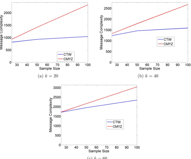
Figure 4.6 Number of messages versus sample size, wherekis the number of sites. 39

Figure 4.8 Number of messages versus number of sites . . . 40

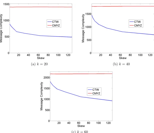
Figure 4.10 Number of messages versus the skew, when sample size is 50. . . 41

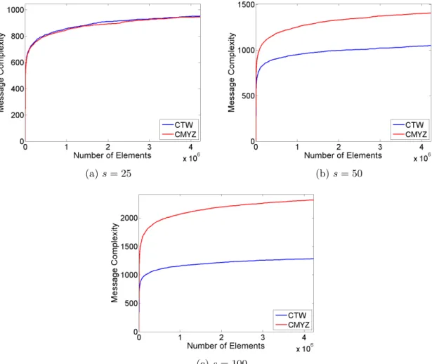
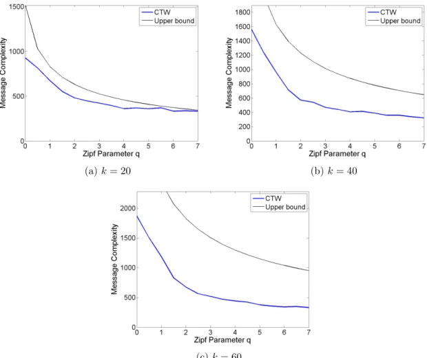
Figure 4.12 Number of messages versus Zipf Distribution variableq, when the sam-ple size is 50. . . 42

Figure 5.2 The communication complexity as a function of number of elements under two different methods of data distribution, “flooding” and “ran-dom”, for 10 sites and a sample size of 5. . . 62

Figure 5.4 The communication complexity as a function of the sample sizesfor 50 sites. . . 63

Figure 5.6 The communication complexity as function of the number of sitesk for a sample size of 20. . . 63

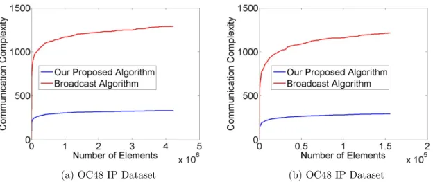
Figure 5.8 The communication complexity by Algorithm Broadcast and our pro-posed method for 10 sites and a sample size of 5. . . 64

Figure 5.10 The communication complexity by Algorithm Broadcast and our pro-posed method on different sample size with 50 sites. . . 65

(9)

Figure 5.12 The communication complexity by Algorithm Broadcast and our pro-posed method on different number of sites (k) with a sample size of 20. . . 65

Figure 5.14 The communication complexity by Algorithm Broadcast and our pro-posed method, as a function of the skew, for 20 sites and a sample size of 20. . . 66

Figure 5.16 The communication complexity by Random Sampling algorithm Tirtha-pura and Woodruff (2011) and our proposed method as a function of number of elements for 20 sites and a sample size of 50 using flooding distribution. . . 67

Figure 5.18 The communication complexity by Random Sampling algorithm Tirtha-pura and Woodruff (2011) and our proposed method as a function of number of elements for 20 sites and a sample size of 50 using Round-Robin data distribution. . . 67

Figure 5.20 The communication complexity sent by Random Sampling algorithm Tirthapura and Woodruff (2011) and our proposed method as a function of number of elements for 20 sites and a sample size of 50 using random data distribution. . . 68

Figure 5.22 The number of messages sent by Random Sampling algorithm Tirtha-pura and Woodruff (2011) and our proposed method as a function of skew for 20 sites and a sample size of 50 using random data distribution. 68

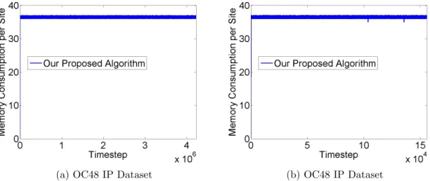
Figure 5.24 Sliding Windows: Memory consumption in each site versus time steps for 40 sites, a sample size of 5, and a sliding window of 150 . . . 70

Figure 5.26 Sliding Windows: Communication complexity versus time steps for 40 sites, a sample size of 5, and a sliding window of 150 . . . 70

Figure 5.28 Sliding Windows: Communication complexity as a function of number of sites for a sample size of 10 and a window size of 100 . . . 71

Figure 5.30 Sliding Windows: Communication complexity as a function of window size for 40 sites and a sample size of 10 . . . 72

(10)

Figure 5.32 Sliding Windows: Communication complexity as a function of number

of sites for 40 sites and a window size of 100 . . . 73

Figure 6.1 The architecture of the unsupervised insider threat detection . . . 77

Figure 6.2 The diagram of Scenario-based Anomaly Detection Framework. . . 79

Figure 6.4 These histograms show the logon hour for selected users in r2 . . . 80

Figure 6.6 These histograms show the logon hour for selected users in r3.1 . . . . 81

Figure 6.22 These histograms show the number of email recipients for selected users in r2 . . . 85

Figure 6.23 These histograms show the number of email recipients for selected users in r3.1 . . . 86

(11)

Figure 6.34 These histograms show the number of email recipients for selected users

in r6.1 . . . 88

Figure 6.38 These histograms show different patterns of removable device usage for selected users in r2 . . . 90

Figure 6.40 These histograms show different patterns of removable device usage for selected users in r3.1 . . . 91

Figure 6.55 The diagram of FSM for scenario 1. . . 96

Figure 6.57 FSM diagrams for attack scenarios in the CERT dataset. . . 104

Figure 6.58 The diagram of the combination of all the FSM. . . 105

Figure 6.60 Evaluation metrics for r2 in CERT datasets . . . 106

Figure 6.62 Evaluation metrics for r3.1 in CERT datasets . . . 107

(12)

(13)

ABSTRACT

With the current explosion in the speed and volume of data, the conventional computation systems are not capable of dealing with large data efficiently. In this project, we do research in the data stream sampling methods and an application on insider threat detection.

The goal of random sampling is to select a subset from the original population so that the subset can represent the whole population. In many real world applications, by sampling a subset from the original population, we can estimate the global statistical properties, such as mean, variance, probability distribution, etc. The goal of random sampling from a distributed stream is to select a subset from the union of the streams such that each element in the distributed stream is sampled with equal probability.

In some cases, the “Heavy Hitters” dominate the random sample. The heavy hitters are the elements with high frequency. The distinct random sample can be applied so that the elements with low frequency can also be seen. Distinct sampling from a distributed stream is proposed to extract a subset from the unique set of the union of the distributed stream. In database query optimization, sampling unique subset from the population is an important task. Random sampling and distinct sampling are among the fundamental techniques and algorithms for large scale data analysis and the query enhancement over database systems. We propose algorithms, theoretical analysis, and experimental evaluations on random sampling and distinct sampling from a distributed stream.

Nowadays, with more and more attacks on the computer systems, it is important to know how we protect our computer systems or classified information from hackers or attackers. Among all the attack or data breaches, more and more cases come from inside of an organiza-tion. It is called “Insider Threat.” In recent reports, malicious insiders are causing enormous damages in organizations. We propose two insider threat detection framework that monitors the system logs and detect anomaly behaviors. We propose a Scenario-based Insider Threat

(14)

Detection method and a Session-based Insider Threat Detection. We implement our framework in Java, and present experimental evaluation on a synthetic dataset.

(15)

CHAPTER 1. INTRODUCTION

With the current explosion in the speed and volume of data, the term “Big Data” has become popular in the computer science community. According to Internet Live Stats1, Twitter has more than 332 million active users per day, with more than 474 million tweets every day. Google receives more than 2.4 billion search requests daily. More than 1.4 EB data is transmitted each day. These data, which arrive in real-time fashion, are called the “Data Stream.” The term “Data Stream” refers to a continuous, possibly time-varying, sequence of data records, in the form of events, messages, tuples, etc. Some applications require to monitor data stream and evaluate important statistical properties from data stream. If Amazon want to know the best selling merchandise in the previous hour, one of the methods is to store the distinct set of elements and their counts in a hash map. But if we want to find the most popular merchandise in the 24-hour window, we need to store billions of entries in the memory. It is not memory and computation efficient. We need a data stream computation algorithm, which is memory and computation efficient, and possibly one-pass.

1.1 Data Stream Sampling

In many cases, data streams are dispersed among different areas of the world. For example, Google has data centers places such as Council Bluffs, USA, Douglas County, USA, Changhua County, Taiwan. The coordinator is responsible for answering the query about the union of the distributed streams. One way is to send to the coordinator whatever the sites observe. However, the transmitted data in local data streams can be large. The network bandwidth is a valuable and limited resource. It is impractical to collect all the data in one site and to

(16)

Figure 1.1: Distributed network model with ksites and a coordinator

compute them in a centralized manner. A new computation model is required under distributed network.

Cormode et al. (2008) has proposed the distributed, continuous streaming model. Figure1.1

shows the architecture of our distributed model with k sites. Each site receives a large volume of data from the local stream,Si. The coordinator responds to queries over the union of local

streams,S=∪k

i=1Si. The main problems in the distributed model are how to answer accurately

at the coordinator at all times and how to minimize the communication cost between sites and the coordinator.

In the distributed computation system, the distributed sites usually send out the summary of necessary information to the coordinator. One of the summary techniques is to sample a subset from the population. Random sampling is a fundamental problem to provide a smaller subset from the population, where the subset is able to present the attributes in the population. Sampling is also one of the tool to provide stream summary, approximate database and search

(17)

query, selectivity estimation, and query planning. To generate a random sample over data streams, one of the problems is the size of streams. The data observed from data stream is enormously large; Facebook, for example, has 510 comments, 293 thousands status updates, and 136 thousands photo uploads every 60 seconds. One of the solutions is to apply distributed network model so that we can divide the load among the data centers. A requirement of distributed random sampling over a distributed stream is raised. An application of distributed data stream is on network routers. Maintaining a random sample from the union of data streams is important to detect the global properties Huang et al. (2007). Estimating the number of distinct elements Cormode and Garofalakis (2005); Cormode et al. (2008) and heavy hitters Babcock and Olston (2003); Keralapura et al. (2006); Manjhi et al. (2005); Yi and Zhang (2009) are also popular problems on distributed data streams.

An alternative aggregation method is distinct random sampling. A distinct random sample is a subset chosen from the set of unique elements in data. The probability of an element to be sampled is independent from its frequency, as long as it is observed so far. It is useful to answer the number of distinct elements or the summary of distinct elements. For example, in network monitoring, we are interested in the number of distinct IPs visiting a specific website. Recall the simple random sampling, where the probability of an element to be sampled is proportional to its frequency. Heavy hitters, those elements with high frequency in data, are favorable for simple random sampling. The higher frequency an element is observed, the more likely the element is to be sampled in simple random sampling. With highly skewed data distribution, a few elements dominate the sample whereas elements with low frequency are ignored. In contrast, a distinct random sample is independent from the element frequency. Low-frequency elements are equally likely to be included in distinct random sample.

Due to this property, distinct random sampling has been found in several applications in database query processing Gibbons (2001), network monitoring Tirthapura et al. (2006), and in detecting anomalous network traffic Venkataraman et al. (2005); a simple random sampling method is not suitable for these applications. Another application of distinct random sampling is query optimizers in commercial relational database systems. Query optimizers enhance the

(18)

choice of query processing strategy by maintaining a d distinct sample of individual database columns Poddar ().

1.2 Insider Threat Detection

For organizations and companies, information security is always a practice to protect their assets from being compromised by outside forces. Along with the growth and the advance in computer technology, cyber security and communication security are gaining importance. Hackers steal information from organizations and companies, causing physical and virtual dam-ages. In 2013, Target faced a hackeing incident, causing loss of credit and debit card records of more than 40 million customers, as well as personal information of 70 million people. Target had to pay 10 million dollars to settle the lawsuit. The loss of Target is not only the cost of lawsuit but also the loss of customers and their confidence. This confidentiality of information is well-known, and many researches has been immersed to the issue.

However, another type of attack is emerging. Insiders, who have permission to access the computer systems within a domain of normal behavior to accomplish their work efficiently, perform malicious activities, including stealth, damage, and modification of secret information. Most of the security defense systems are designed to defend attacks from outside, not inside. The attack from insiders is hard to detect. According to a speech in RSA Conference Richards (2013) based on the survey over 10 years period, “The average cost per incident is $412,000, and the average loss per industry is $15 million over ten years. In several instances, damages reached more than $1 billion.” The cost of insider attack can be so large; the attack of insider is hard to detect. There are some case studies. In comparison with intruders, insiders have more sophisticated knowledge about the computation systems and data structure. Gunasekhar, Rao, and Basu study the definition of different type of insiders, discover the difficulties in detection, and propose ways to prevent. In their study, the types of insiders can be (1) Pure insiders, (2) Insider Associates, (3) Insider affiliates, and (4) Outside affiliates. The pure insiders are the employees. The insider associates are the other employees who have physical access to the computers, such as security guards, and janitors.

(19)

The insider affiliates are the friends or spouses of employees, who have chances to access to the computer when visiting. Outside affiliates can access into the network via unprotected wireless network. Research on insider threat have several categories: the philosophy of malicious insiders, the behavior patterns and motivations of malicious insiders, and the detection of malicious insiders. Randazzo et al. (2005) proposed six findings on their analysis on 80 cases.

• The executions by criminals are “low and slow.” In average, the time elapse almost 32 months to be detected by the victim organization.

• The means of insiders were not very sophisticated. The role they served are seldom technical, or their fraud behaviors are not explicitly technical.

• The frauds by manager are different from the ones by non-manager in their damage and duration.

• Most cases don’t involved with collusion.

• An audit, customer complaints, or coworker suspicion are the three common detection ways of insider incidents.

• The target of committing fraud is on personal identifiable information (PII).

In this project, we work on different approaches toward the discovery of malicious insiders. We propose a Session-based Insider Threat Detection and a Scenario-based Insider Threat Detection. The session-based insider threat detection provides a high-level view on users’ behavior pattern. We segment the system logs of a user into a smaller chunk, called Session. By comparing the current session with the history sessions, we can deviate anomaly session from the normal sessions. The scenario-based insider threat detection starts from knowing insider’s attack scenarios. Malicious insiders have their intention, either stealing classified information from the organization or causing damage to organizations reputation. An attack scenario describes how the malicious insider achieve their intention. By understanding their attack scenarios, we can detect if the behavioral sequence of a user matches any attack scenario. An experimental evaluation is presented to compare the performance of the two approaches.

(20)

CHAPTER 2. CONTRIBUTION

2.1 Random Sampling from a Distributed Stream

Our main contributions are a simple algorithm for sampling without replacement from a distributed stream, as well as a matching lower bound showing that the message complexity of our algorithm is optimal. The message complexity is the number of message transmission between sites and the coordinator. The algorithm is easy to implement, and as our experiments show, has very good practical performance.

Algorithm: We present an algorithm that uses an expected O

klog(n/s) log(1+(k/s))

number of mes-sages for continuously maintaining a random sample of size sfromk distributed data streams of total sizen. Note that ifs < k/8, this number isO

klog(n/s) log(k/s)

, while ifs≥k/8, this number is O(slog(n/s)). The memory requirement at the coordinator is s words. The remote sites in our scheme store a single machine word and use constant time per stream update, both of which are clearly optimal.

Lower Bound: We also show that any correct protocol which succeeds with constant proba-bility must send Ω_log(1+(klog(n/s_k/s)₎₎ messages with constant probability. This also yields a bound of Ω

on the expected message complexity of any correct protocol, showing that the expected number of messages sent by our algorithm is optimal, up to constant factors.

Impact of Skew: The algorithm and lower bound as discussed do not assume any distribution on the numbers of elements that arrive at the different sites. The worst case message complexity arises in the setting where different sites receive nearly the same number of elements. In a practical setting, however, it is common to have a skewed distribution of the arrivals at different local streams. For example, traffic sensors posted on streets observing cars pass by may see different volumes of activity depending on how busy the streets are. It is important

(21)

to consider the performance in the skewed case when the different streams Si are of different

sizes.

To measure the performance of our algorithm in the presence of skew, we considered the following model of data arrival. Suppose a set of probabilities pi, i= 1. . . k, one per site, such

that Pk_i₌₁pi = 1. Each arrival into the system is sent to stream Si with a probability of pi. The pis need not be equal, so that the numbers of elements seen by different sites can be

significantly different from each other.

We show that under such a model, our algorithm has a message complexity ofO slog(n/s)P i,pi6=0 1 log(2 pi) . Note that the algorithm remains the same as in the worst case analysis, but the message

com-plexity is different, due to the assumed input model.

The message complexity under skew can be much smaller than the upper bound for general case. For example, suppose there were only five sites receiving data, and the rest did not receive any data. Further, suppose we want a sample of size 1. We have pi = 0.2 for i= 1. . .5, and pi = 0, i > 5. In such a case the message complexity of our algorithm is only O(logn). In

contrast, the worst case upper bound for a sample size of 1 isO

klogn

logk

.

In another case, suppose thatp1= 1−c(k−1)/n, andpi =c/nfori≥2, wherecis a constant

independent ofn. This models the case when one site receives a majority of elements, and each of the other sites receives only aboutcelements. In such a case, the message complexity of our algorithm isO(k+ logn), to be contrasted with the general bound ofOk_loglog_kn.

Experimental Evaluation: We conducted an experimental study evaluating the message cost of our algorithm, comparing with the cost of the algorithm from Cormode et al. (2012). We observe that the number of messages in our algorithm has a linear dependence on the number of sites and sample size. In general, our algorithm achieves better performance than the algorithm from Cormode et al. (2012). The benefit is especially clear when the required sample size is high. In the presence of skew in data, our algorithm shows significantly improved performance when compared with the case of no skew.

Sampling With Replacement: We also show how to modify our protocol to obtain a ran-dom sample of size s chosen with replacement. The message complexity of this protocol is

O

k

log(2+(k/(slogs)))+slogs

logn

(22)

2.2 Distinct Random Sampling from a Distributed Stream

We make the following contributions. Let k denote the number of distributed sites, s the desired sample size, and dthe total number of distinct elements in the distributed stream.

• We present a distributed algorithm for continuously maintaining a distinct sample with-out replacement from a distributed stream. The expected message complexity of the algorithm isO kslnde_s

. When a query is posed at the central coordinator, it responds with a distinct sample of size min{s, d} from the set of all elements seen so far in the stream.

• We present a matching lower bound showing that anyalgorithm for continuously main-taining a distinct sample without replacement from the distributed stream must have a message complexity of Ω kslnde_s. In other words, the message complexity of our algorithm is optimal, to within a constant factor.

• We present an extension for continuously maintaining a distinct sample with replacement from a distributed stream. We show that the message complexity of this algorithm is bounded byO kslnde_s, and that this is optimal to within a constant factor.

• We present an extension to sampling from a sliding window of the distributed stream. We show this algorithm is also near-optimal in its message complexity through an appropriate lower bound.

• We implemented our algorithm and evaluated its practical performance. We found that our algorithms are easy to implement and provide a message complexity that is typically much better than the worst case bounds that we derive.

Comparison with Simple Random Sampling

It is interesting to compare the message complexity of distributed distinct sampling (DDS) to that of distributed simple random sampling (DRS). From previous work Cormode et al. (2012); Tirthapura and Woodruff (2011), it is known that the message complexity of DRS for a sample sizesforntotal elements distributed overksites increases as approximately max{k, s}log(n/s)

(23)

1 _{In contrast, the message cost of DDS increases as} _k_·_s_·_log(_d/s_{), where} _k _{is the number of} sites,dthe total number of distinct elements, andsthe sample size. The message complexity of DDS is inherently larger than that of DRS ifd(the number of distinct elements in the stream) is comparable to n(the total number of elements in the stream).

To understand the reason for this difference, note that in DRS, when n elements have already been received in the system, the probability of a new element being selected into the sample decreases as s/n. In case of DDS, the probability of a new element being selected into the sample decreases ass/d, wheredis the number of distinct elements received by the system. Due to the possibility of the same element appearing at different sites at a similar time, many sites may be “fooled” into sending messages to the coordinator after simultaneously observing the same element, and hence more messages may be communicated between the sites and the coordinator in DDS. Our lower bound shows that this is not an artifact of an inferior algorithm for DDS. Instead, greater coordination is inherently necessary for DDS than for DRS.

In our empirical experiment result, we observe that the message complexity of DDS is higher than DRS when using flooding, round-robin, and random data distribution. Especially, when using flooding distribution method, the DDS has message complexity 5 times higher than DRS for 20 sites and a sample size of 50. When receiving the same element, the sites of DDS send out messages if the element is to be sampled. The sites of DRS behave differently. Each site samples the same element with probability of _ns. It makes the difference between DRS and DDS.

2.3 Insider Threat Detection from Log Streams

Our main contribution is developing a scenario-based anomaly detection framework. A scenario is a sequence of events, describing how a malicious insider attacks an organization. For example, Eric, a malicious insider, logs on at 9PM, searches for classified files, copies files into an USB stick, and then logs off. We discover the anomaly events from the logs, and

1_{The exact expression is Θ}klog(n/s) log(k/s)

ifs < k/8 and Θ(slog(n/s)) ifs≥k/8. This message complexity is tight up to a constant factor, due to matching lower bounds.

(24)

transform the anomaly event sequence into a string, L. Scenario, Si, is formatted as a general

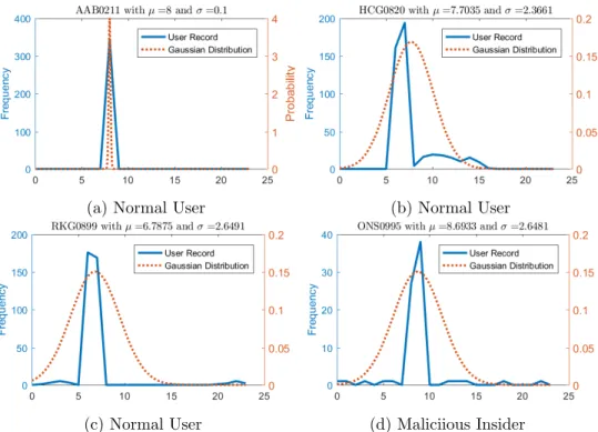
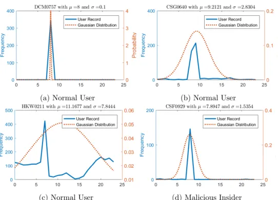
expression. If there is a match betweenLandS_i, we can report anomaly for the event sequence. However, the anomaly events are nondeterministic. Logon hour, for example, is variant among different users. It may be varied because of different working customs or work shifts. A deterministic logon time range is not feasible for our application. A probability model is applied to each user. We build up a probability model based on user’s history events, and detect anomaly based on the model.

We implement our framework in Java, and evaluate its performance in real world. Our framework detects the most events by malicious insiders from our reported events and from all malicious insiders in the answer. We also detect the most malicious users from the dataset.

(25)

CHAPTER 3. LITERATURE REVIEW

3.1 Random Sampling from a Distributed Stream

Obtaining a random sample from the union of distributed stream is required. Reservoir Sampling Vitter (1985); Knuth (1981) algorithm (where this algorithm is attributed to Water-man) is generalized to this problem. Our work generalizes the classic algorithm to the setting of multiple distributed streams. We compare our algorithm with the algorithm proposed by Cormode et al. (2012), short handed as CMYZ. The performance is evaluated by the message complexity and memory consumption. The message complexity is the number of messages between distributed sites, and the memory consumption is the coordinator and the number of data elements stored in the sites and the coordinator respectively. The message complexity of CMYZ is reported as Ohklog_k/sn+slogni, where k is the number of sites, s is the sample size, andnis the number of elements observed so far. The comparison of our work and CMYZ is shown in Table3.1.

In additional to CMYZ, there are other researches in the continuous distributed streaming model, including estimating frequency moments and counting the number of distinct elements Cormode and Garofalakis (2005); Cormode et al. (2008), and estimating the entropy Arack-aparambil et al. (2009). Stream sampling has a long history of research, starting from the popular reservoir sampling algorithm, attributed to Waterman (see Algorithm R from Vitter

Table 3.1: Summary of Our Results for Message Complexity of Sampling Without Replacement

Upper Bound Lower Bound

Our Result CMYZ Cormode et al. (2012)

s < k₈ O klog(n/s) log(k/s) O klogn log(k/s) Ω klog(n/s) log(k/s) s≥ k

(26)

(1985)) that has been known since the 1960s. Follow-up work includes speeding up reservoir sampling Vitter (1985), weighted reservoir sampling Efraimidis and Spirakis (2006), sampling over a sliding window and stream evolution Braverman et al. (2012); Xu et al. (2008); Babcock et al. (2002); Gemulla and Lehner (2008); Aggarwal (2006a). Stream sampling has been used extensively in large scale data mining applications, see for example Pavan et al. (2013); Dash and Ng (2006); Malbasa and Vucetic (2007); Aggarwal (2006b). Stream sampling under sliding windows has been considered in Braverman et al. (2009); Babcock et al. (2002). Deterministic algorithms for finding the heavy-hitters in distributed streams, and corresponding lower bounds for this problem were considered in Yi and Zhang (2009). Stream sampling under sliding win-dows over distributed streams has been considered in Cormode et al. (2010a). Continuous random sampling from the set of distinct elements in a stream has been considered in Chung and Tirthapura (2015). The question of how to process a “sampled stream”,i.e. once a stream has been sampled, is considered in McGregor et al. (2012).

A model of distributed streams related to ours was considered in Gibbons and Tirthapura (2001, 2002, 2004). In this model, the coordinator was not required to continuously maintain an estimate of the required aggregate, but when the query was posed to the coordinator, the sites would be contacted and the query result would be constructed. In their model, the coordinator could be said to be “reactive”, whereas in the model considered in this paper, the coordinator is “pro-active”.

3.2 Distinct Random Sampling from a Distributed Stream

There is a growing literature on algorithms for continuous distributed monitoring, starting from the basic “countdown problem” Cormode et al. (2008), frequency moments Woodruff and Zhang (2012); Cormode et al. (2008), entropy Arackaparambil et al. (2009), heavy-hitters and quantiles Yi and Zhang (2013), geometric methods for monitoring Sharfman et al. (2007); Giatrakos et al. (2012), and often, matching lower bounds Woodruff and Zhang (2012). For a recent survey on results in this model, see Cormode (2013). A survey of sampling on streams appears in Lahiri and Tirthapura (2009).

(27)

The closest prior work is the work on algorithms and lower bounds for distributed random sampling Tirthapura and Woodruff (2011); Cormode et al. (2012). While the problems are different, our algorithm for DDS on an infinite window is essentially an adaptation of the DRS algorithm from Tirthapura and Woodruff (2011) with a few important differences: one is that our algorithm uses sampling based on a randomly chosen hash function while the algorithm for DRS samples based on independent random bits. Further, our algorithm employs additional data structures to prevent duplicate messages from a site to the coordinator due to observing the same element, this is not necessary for simple random sampling. The analysis of the message complexity for the DRS and the DDS algorithms are different. The lower bound arguments for the two problems (DRS and DDS) are also substantially different from each other. Our analysis of the lower bound on message cost of any algorithm for DDS uses methods, that to our knowledge, have not been applied to the continuous distributed streaming model.

3.3 Insider Threat Detection from Log Streams

The researches in insider threat are diverse among different fields. Psychologists research in the detection of malicious insiders by behavior models Greitzer et al. (2012); Berk et al. (2012), psychological profiling Axelrad et al. (2013). Shaw and Fischer (2005) propose the analysis and overview of 10 types of trust betrayal. Based on their observations, they offer 8 cases applied to insider threat. Schultz proposes a framework for predicting insider attacks by defining attack related behavior and symptoms. Gates et al. (2014) propose their work on normal user profile building, and information theft and leakage detection from file access logs. Duncan et al. (2012) research in the applicability of current insider threat definitions and classifications in the cloud environment.

Wave (), one of the insider threat mitigation software, focuses on specifically on data loss prevention. Data encryption, automated remote backup, and document tagging are used to prevent malicious insiders to deface, delete, or exfiltrate sensitive organization information. Another approaches such as Raytheon’s SureView () apply compilation and analysis on multiple sources of information on user behaviors. Other technologies, such as Palisade (), Prelert (), and Securonix (), identify malicious behaviors from malicious insiders by characterizing network and

(28)

user behaviors. Murphy et al. (2012); Berk et al. (2012) proposed BANDIT system, applying 10-step common-sense approach to limit the damage from malicious insiders.

As email becomes one of the common communication tools, the malicious usage of email service gets severe. Several works have been devoted into the analysis and detection of malicious usage of email, including spam or junk email detection. Machine learning techniques have been applied to this era, e.g. Bayesian or Naive Bayessian classifier Sahami et al. (1998); Meyer and Whateley (2004); Wang et al. (2015), decision tree Ghosh et al. (2012a), and kNN Harisinghaney et al. (2014). The algorithms also apply to Short Message Service (SMS) Cormack et al. (2007); G´omez Hidalgo et al. (2006). As the social network services get popular, the misuse of social networks is an issue. Several works Boykin and Roychowdhury (2005); Tan et al. (2013); Ghosh et al. (2012b); Yardi et al. (2009) have been proposed to detect spam messages in social network. All the works above review the content of the messages and detect the spams by the word frequency features or TF-IDF.

Finite state machine is also applied in insider anomaly detections. Ho and Lee () proposed a insider threat framework using FSM. They simulate insider threat situations by building several experiments. Greitzer et al. (2008) propose an insider threat prediction framework from employees’ psychosocial data, and with cybersecurity audit data. Ambre and Shekokar (2015) build up a probabilistic approach and incorporate with log analysis and event correlation on detecting anomaly insiders events. Upon receiving system logs, they first filter out unwanted events based rules. A probability of an intrusion behavior given an event is calculated by Bayessian theorem, and is used to determine if the given event is anomaly.

(29)

PART I

(30)

CHAPTER 4. DISTRIBUTED RANDOM SAMPLING ON A DATA STREAM

4.1 Model

The coordinator node is assumed to be different from any of the sites. The coordinator does not observe a local stream, but all queries for a random sample arrive at the coordinator. It is straightforward to modify our algorithms for the case when the coordinator also observes a local stream. Let S = ∪n

i=1Si be the entire stream observed by the system, and note that

the total number of elements n = |S|. The sample size s supplied to the coordinator and to the sites during initialization. The task of the coordinator is to continuously maintain a random samplesof size min{n, s}consisting of elements chosen uniformly at random without replacement fromS.

We assume a synchronous communication model, where the system progresses in “rounds”. In each round, each site can observe one element (or none), and send a message to the coor-dinator, and receive a response from the coordinator. The coordinator may receive up to k

messages in a round, and respond to each of them in the same round. This model is essentially identical to the model assumed in previous work Cormode et al. (2010a).

The sizes of the different local streams at the sites, their order of arrival, and the inter-leaving of the streams at different sites, can all be arbitrary. The algorithm cannot make any assumption about these. For instance, it is possible that a single site receives a large number of elements before a different site receives its first element. It is also possible that all sites receive elements streams that are of the same size and whose elements arrive in the same rounds. In Section 4.5, we analyze the performance of the algorithm under certain specific input

(31)

distri-butions. However, the algorithm still remains the same, and does not depend on the input distribution.

Note that what matters for the algorithm is the global ordering of the stream items by their time of arrival onto one of the sites. The “speed” of the stream, i.e., how long it takes for the next item to arrive on a site does not play any role in the complexity of our algorithm, which is concerned with the total number of messages transmitted.

4.2 Algorithm

Algorithm Intuition: The idea in the algorithm is as follows. Each site associates a random weight with each element that it receives. The coordinator then maintains the set P of s

elements with the minimum weights in the union of the streams at all times, and this is a random sample of S. This idea is similar to the spirit in all centralized reservoir sampling algorithms. Reservoir sampling is a method for maintaining a random item from a stream of items, while using memory that is small when compared with the size of the stream. Indeed, one way to implement reservoir sampling is to assign a random weight to each stream item and maintain the item with the minimum weight. In a distributed setting, the interesting aspect is at what times do the sites communicate with the coordinator, and vice versa.

In our algorithm, the coordinator maintains u, which is the s-th smallest weight so far in the system, as well as the sample P, consisting of all the elements that have weight no more than u. Each site needs only maintain a single value ui, which is the site’s view of the s-th

smallest weight in the system so far. Note that it is too expensive to keep the view of each site synchronized with the coordinator’s view at all times – to see this, note that the value of the

s-th smallest weight changes O(slog(n/s)) times, and updating every site each time the s-th minimum changes takes a total ofO(sklog(n/s)) messages.

In our algorithm, when site isees an element with a weight smaller than ui, it sends it to

the central coordinator. The coordinator updatesu and P, if needed, and then replies back to

i with the current value of u, which is the true minimum weight in the union of all streams. Thus each time a site communicates with the coordinator, it makes a change to the random sample, or, at least, gets to refresh its view of u.

(32)

The algorithm at each site is described in Algorithms 1 and 2. The algorithm at the coordinator is described in Algorithm3.

Algorithm 1:Initialization at Sitei.

1 /* ui is site i’s view of the s-th smallest weight in the union of all streams so far. Note this may ‘‘lag’’ the value stored at the

coordinator, in the sense that it may not agree with the s-th smallest

weight held by the coordinator. */

2 ui←1;

Algorithm 2:When Siteireceives element e.

1 Let w(e) be randomly chosen weight between 0 and 1; 2 if w(e)< u_i then

3 Send (e, w(e)) to the Coordinator; 4 Receiveu0 from Coordinator;

5 Setu_i ←u0;

Algorithm Correctness: Lemmas 1 and 2establish the correctness of the algorithm.

Lemma 1. (1) Ifn≤s, then the set P at the coordinator contains all the (e, w) pairs seen at all the sites so far. (2) If n > s, then P at the coordinator consists of the s (e, w) pairs such that the weights of the pairs in P are the smallest weights in the stream so far.

Proof. The variableuis stored at the coordinator, anduiis stored at sitei. First we note that

the variables u and ui are non-increasing with time; this can be verified from the algorithms.

Next, we note that for every ifrom 1 tillk, at every round, ui ≥u. This can be seen because

initially, ui =u= 1, andui changes only in response to receivingu from the coordinator.

Thus, if fewer than s elements have appeared in the stream so far,u is 1, and henceui is

also 1 for each sitei. The next element observed in the system is also sent to the coordinator. Thus, ifn≤s, then the setP consists of all elements seen so far in the system.

Next, we consider the case n > s. Note that u maintains the s-th smallest weight seen at the coordinator, and P consists of the s elements seen at the coordinator with the smallest weights. We only have to show that if an element e, observed at site i is such thatw(e) < u

(33)

Algorithm 3:Algorithm at Coordinator.

1 /* The random sample P consists of tuples (e, w) where e is an element, and w the weight, such that the weights are the s smallest among all

the weights so far in the stream */

2 P ← ∅;

3 /* u is the value of the s-th smallest weight in the stream observed so far. If there are less than s elements so far, then u is 1. */

4 u←1;

5 while true do

6 if a message (e_i, u_i) arrives from site ithen 7 if ui < uthen

8 Insert (ei, ui) intoP; 9 if |P|> s then

10 Discard the element (e, w) fromP with the largest weight;

11 Updateu to the current largest weight in P (which is also the s-th

smallest weight in the entire stream);

12 Sendu to sitei;

13 if a query for a random sample arrives then

14 returnP

and ifw(e) < u, then it must be true thatw(e)< ui, and in this case, (e, w(e)) is sent to the

coordinator.

Lemma 2. At the end of each round, sampleP at the coordinator consists of a uniform random sample of sizemin{n, s} chosen without replacement fromS.

Proof. In case n ≤ s, then from Lemma 1, we know that P contains every element of S. In case n > s, from Lemma 1, it follows that P consists of s elements with the smallest weights from S. Since the weights are assigned randomly, each element inS has a probability of _ns of belonging inP, showing that this is an uniform random sample. Since an element can appear no more than once in the sample, this is a sample chosen without replacement.

4.3 Analysis of the Algorithm (Upper Bound)

(34)

For the sake of analysis, we divide the execution of the algorithm into “epochs”, where each epoch consists of a sequence of rounds. The epochs are defined inductively. Let r > 1 be a parameter, which will be fixed later. Recall that u is the s-th smallest weight so far in the system (if there are fewer than selements so far,u= 1). Epoch 0 is the set of all rounds from the beginning of execution until (and including) the earliest round whereuis 1_r or smaller. Let

mj denote the value of u at the end of epoch j−1. Epoch j consists of all rounds subsequent

to epoch (j−1) until (and including) the earliest round when u is mj

r or smaller. Note that

the algorithm does not need to be aware of the epochs, and this is only used for the analysis. Suppose we call the original distributed algorithm described in Algorithms 3 and 2 as AlgorithmA. For the analysis, we consider a slightly different distributed algorithm, Algorithm

B, described below. Algorithm B is identical to Algorithm A except for the fact that at the beginning of each epoch, the value u is broadcast by the coordinator to all sites.

While Algorithm A is natural, AlgorithmB is easier to analyze. We first note that on the same inputs, the value ofu(andP) at the coordinator at any round in AlgorithmB is identical to the value of u (and P) at the coordinator in Algorithm A at the same round. Hence, the partitioning of rounds into epochs is the same for both algorithms, for a given input. The correctness of Algorithm B follows from the correctness of AlgorithmA. The only difference between them is in the total number of messages sent. In B we have the property that for all i from 1 to k, ui = u at the beginning of each epoch (though this is not necessarily true

throughout the epoch), and for this, B has to pay a cost of at leastk messages in each epoch.

Lemma 3. The number of messages sent by AlgorithmAfor a set of input streamsSi, i= 1. . . k

is never more than twice the number of messages sent by Algorithm B for the same input. Proof. Consider sitevin a particular epoch j. In AlgorithmB,vreceivesmj at the beginning

of the epoch through a message from the coordinator. In AlgorithmA,v may not knowmj at

the beginning of epoch j. We consider two cases.

Case I: v sends a message to the coordinator in epoch j in AlgorithmA. In this case, the first time v sends a message to the coordinator in this epoch, v will receive the current value of u, which is smaller than or equal to mj. This communication costs two messages, one in

(35)

each direction. Henceforth, in this epoch, the number of messages sent in Algorithm A is no more than those sent inB. In this epoch, the number of messages transmitted to/fromv inA

is at most twice the number of messages as inB, which has at least one transmission from the coordinator to site v.

Case II:v did not send a message to the coordinator in this epoch, in AlgorithmA. In this case, the number of messages sent in this epoch to/from sitev in Algorithm Ais smaller than in Algorithm B.

(36)

Let ξ denote the total number of epochs. Lemma 4. If r≥2, E[ξ]≤ log(n/s) logr + 2 Proof. Letz= log(n/s) logr

. First, we note that in each epoch,udecreases by a factor of at least

r. Thus after (z+`) epochs, u is no more than _rz+`1 = (

s n) 1 r`. Thus, we have Pr[ξ≥z+`]≤Pr u≤s n 1 r`

LetY denote the number of elements (out ofn) that have been assigned a weight of _nrs` or lesser. Y is a binomial random variable with expectation _rs`. Note that if u≤

s

nr`, it must be true thatY ≥s.

Pr[ξ ≥z+`]≤Pr[Y ≥s]≤Pr[Y ≥r`E[Y]]≤ 1 r`

where we have used Markov’s inequality. Since ξ takes only positive integral values,

E[ξ] = X i>0 Pr[ξ ≥i] = z X i=1 Pr[ξ ≥i] +X `≥1 Pr[ξ≥z+`] ≤ z+X `≥1 1 r` ≤z+ 1 1−1/r ≤z+ 2

where we have assumed r≥2.

Letnj denote the total number of elements that arrived in epochj. We haven=Pξ_j−₌₀1nj.

Let µ denote the total number of messages sent during the entire execution. Let µj denote

the total number of messages sent in epochj and Xj the total number of messages sent from

the sites to the coordinator in epoch j. µj is the sum of two parts, (1)k messages sent by the

coordinator at the start of the epoch, and (2) twice the number of messages sent from the sites to the coordinator.

(37)

µj =k+ 2Xj (4.1) µ= ξ−1 X j=0 µj =ξk+ 2 ξ−1 X j=0 Xj (4.2)

For each κ= 1. . . nj in epochj, we define a 0-1 random variable Yκ as follows. Yκ = 1 if

observing the κ-th element in the epoch resulted in a message being sent to the coordinator, and Yκ = 0 otherwise. Xj = nj X κ=1 Yκ (4.3)

Let F(η, α) denote the eventnj =η and mj =α. The following Lemma gives a bound on

a conditional probability that is used later.

Lemma 5. For each κ= 1. . . nj−1

Pr[Yκ = 1|F(η, α)]≤

α−α/r

1−α/r

Proof. Suppose that thej-th element in the epoch was observed by sitev. For this element to cause a message to be sent to the coordinator, the random weight assigned to it must be less thanuv at that instant. Conditioned on mj =α,uv is no more than α.

Note that in this lemma we exclude the last element that arrived in epochj, thus the weight assigned to element j must be greater than α/r. Thus, the weight assigned to j must be a uniform random number in the range (α/r,1). The probability this weight is less than the current value of uv is no more than α

−α/r

1−α/r, sinceuv ≤α.

Lemma 6. For each epoch j

E[Xj]≤1 + 2rs

Proof. We first obtain the expectation conditioned onF(η, α), and then remove the condition-ing. From Lemma5 and Equation4.3 we get:

(38)

E[Xj|F(η, α)] ≤ 1 +E " ( η−1 X κ=1 Yκ)|F(η, α) # ≤ 1 + η−1 X κ=1 E[Yκ|F(η, α)] ≤ 1 + (η−1)α−α/r 1−α/r.

Usingr≥2 andα≤1, we get: E[Xj|F(η, α)]≤1 + 2(η−1)α.

We next consider the conditional expectation E[Xj|mj =α].

Using Lemma7, we get

E[Xj|mj =α]≤1 + 2α rs α −1 ≤1 + 2rs Since E[Xj] =E[E[Xj|mj =α]], we have E[Xj]≤E[1 + 2rs] = 1 + 2rs. Lemma 7. E[nj|mj =α] = rs α

Proof. Recall that nj, the total number of elements in epoch j, is the number of elements

observed till the s-th minimum in the stream decreases to a value that is less than or equal to

α/r.

Let Z denote a random variable that equals the number of elements to be observed from the start of epoch j till s new elements are seen, each of whose weight is less than or equal

(39)

to α/r. Clearly, conditioned on mj = α, it must be true that nj ≤ Z. For δ = 1 to s, let Zδ denote the number of elements observed from the state when (δ−1) elements have been

observed with weights that are less thanα/r till the state whenδ elements have been observed with weights less than α/r. Zδ is a geometric random variable with parameterα/r.

We have Z = Ps_δ₌₁Zδ and E[Z] = Psδ=1E[Zδ] = sr_α. Since E[nj|mj =α] ≤ E[Z], the

lemma follows. Lemma 8. E[µ]≤(k+ 4rs+ 2) log(n/s) logr + 2

Proof. Using Lemma6 and Equation4.1, we get the expected number of messages in epochj:

E[µj]≤k+ 2(2rs+ 1) =k+ 2 + 4rs

Note that the above is independent of j. The proof follows from Lemma4, which gives an upper bound on the expected number of epochs.

Theorem 1. The expected message complexity E[µ]of our algorithm is as follows.

I: If s≥ k 8, then E[µ] =O slog n s II: If s < k₈, then E[µ] =O klog(n s) log(k s)

Proof. We note that the upper bounds on E[µ] in Lemma 8 hold for any value ofr≥2. Case I:s≥ k

8. In this case, we setr= 2. From Lemma 8,

E[µ] ≤ (8s+ 8s+ 2) log(n/s) log 2 = (16s+ 2) logn s = O slog n s

Case II:s < k₈. We minimize the expression in the statement of Lemma8by settingr= ₄k_s, and get: E[µ] =O klog(n s) log(k s) .

(40)

4.4 Lower Bound

Theorem 2. For a constant q,0 < q < 1, any correct protocol must send Ω

messages with probability at least1−q, where the probability is taken over the protocol’s internal randomness.

Proof. Let β = (1 + (k/s)). Define ξ = Θ_log(1+(log(n/s_k/s)₎₎ epochs as follows: in the j-th epoch,

j∈ {0,1,2, . . . , ξ−1}, there areβj−1kglobal stream updates, which can be distributed among thek servers in an arbitrary way.

We consider a distribution on orderings of the stream updates. Namely, we think of a totally-ordered stream 1,2,3, . . . , n of n updates, and in the j-th epoch, we randomly assign the βj−1k updates among the k servers, independently for each epoch. Let the randomness used for the assignment in thej-th epoch be denotedσj.

Consider the global stream of updates 1,2,3, . . . , n. Suppose we maintain a sample setP ofsitems without replacement. We letP_κ denote a random variable indicating the value ofP after seeingκupdates in the stream. We will use the following lemma about reservoir sampling.

Lemma 9. For any constant q,0< q <1, there is a constant C0=C0(q)>0 for which

• P changes at least C0slog (n/s) times with probability at least 1−q, and

• If s < k/8 and k = ω(1) and ξ = ω(1), then with probability at least 1−q/2, over the choice of {P_κ}, there are at least (1−(q/8))ξ epochs for which the number of times P

changes in the epoch is at least C0slog(1 + (k/s)).

Proof. Consider the stream 1,2,3, . . . , n of updates. In the classical reservoir sampling algo-rithm Knuth (1981), P is initialized to{1,2,3, . . . , s}. Then, for eachκ > s, theκ-th element is included in the current sample setP_κ with probabilitys/κ, in which case a random item in Pκ−1 is replaced withκ.

For the first part of Lemma 9, let Xκ be an indicator random variable if κ causes P to

change. Let X = Pn

κ=1Xκ. Hence, E[Xκ] = s/κ for all κ, and E[X] = Hn−Hs, where Hκ = lnκ+O(1) is the κ-th Harmonic number. Then all of the Xκ, κ > s are independent

(41)

indicator random variables. It follows by a Chernoff bound that Pr[X <E[X]/2] ≤ exp(E[X]/8)≤exp(−(lnn/s)/8) ≤ s n 1/8 .

For anys=o(n), this is less than any constantq, and so the first part of Lemma9 follows sinceE[X]/2 = 1/2·ln(n/s).

For the second part of Lemma 9, consider the j-th epoch, j > 0, which contains βj−1k

consecutive updates. LetYj be the number of changes in this epoch. ThenE[Yj] =slnβ+O(1).

Since Yj can be written as a sum of independent indicator random variables, by a Chernoff

bound,

Pr[Yj <E[Yj]/2] ≤ exp(−E[Yj]/8)

≤ exp(−(slnβ+O(1))/8)

≤ 1

βs/8.

Hence, the expected number of epochs j for whichYj <E[Yj]/2 is at mostPξ_j−₌₁1_βs/81 , which is o(ξ) since we’re promised that s < k/8 and k =ω(1) and ξ =ω(1). By a Markov bound, with probability at least 1−q/2, at most o(ξ/q) = o(ξ) epochs j satisfy Yj ≥ E[Yj]/2. It

follows that with probability at least 1−q/2, there are at least (1−q/8)ξ epochs ifor which the number Yj of changes in the epoch j is at leastE[Yj]/2≥ 1₂slnβ, as desired.

Corner Cases: When s ≥ k/8, the statement of Theorem 7 gives a lower bound of Ω(slog(n/s)). In this case Theorem 7 follows immediately from the first part of Lemma 9

since the changes implied by the first part Lemma9inP must be communicated to the central coordinator. Hence, in what follows we can assumes < k/8. Notice also that ifk=O(1), then

klog(n/s)

log(1+(k/s)) =O(slog(n/s)), and so the theorem is independent ofk, and follows simply by the

first part of Lemma9. Notice also that ifξ =O(1), then the statement of Theorem7amounts to proving an Ω(k) lower bound, which follows trivially since every site must send at least one message.

(42)

Thus, in what follows, we may apply the second part of Lemma 9.

Main Case: Let C > 0 be a sufficiently small constant, depending on q, to be determined below. Let Π be a possibly randomized protocol, which with probability at least q, sends at mostCkξ messages. We show that Π cannot be a correct protocol.

Letτ denote the random coin tosses of Π, i.e., the concatenation of random strings of allk

sites together with that of the central coordinator.

LetEbe the event that Π sends less thanCkξmessages. By assumption, Prτ[E]≥q.Hence,

it is also the case that

Pr

τ,{Pj},{σj}

[E]≥q.

For a sufficiently small constant C0 >0 that may depend onq, let F be the event that there are at least (1−(q/8))ξ epochs for which the number of times P changes in the epoch is at leastC0slog(1 + (k/s)). By the second part of Lemma9,

Pr

τ,{Pj},{σj}

[F]≥1−q/2.

It follows that there is a fixing of τ =τ0 as well as a fixing ofP0,P1, . . . ,Pξ to P00, P10, . . . , Pξ0

for which F occurs and

Pr {σj}

[E |τ =τ0, (P₀,P₁, . . . ,P_ξ) = (P₀0, P₁0, . . . , P_ξ0)] ≥q−q/2 =q/2.

Notice that the three (sets of) random variables τ,{Pj},and {σj} are independent, and so in

particular,{σj} is still uniformly random given this conditioning.

By a Markov argument, if event E occurs, then there are at least (1−(q/8))ξ epochs for which at most (8/q)·C·k messages are sent. If events E and F both occur, then by a union bound, there are at least (1−(q/4))ξ epochs for which at most (8/q)·C·kmessages are sent and S changes in the epoch at least C0slog(1 + (k/s)) times. Call such an epochbalanced.

Let j∗ be the epoch which is most likely to be balanced, over the random choices of{σj},

(43)

are balanced if E and F occur, and conditioned on (P0,P1, . . . ,Pξ) = (P00, P10, . . . , Pξ0) eventF

does occur, andE occurs with probability at least q/2 given this conditioning, it follows that

Pr {σj}

[j∗ is balanced | τ =τ0, (P₀,P₁, . . . ,P_ξ) = (P₀0, P₁0, . . . , P_ξ0)] ≥q/2−q/4 =q/4.

The property ofj∗ being balanced is independent of σj0 forj06=j∗, so we also have

Pr σj∗ [j∗ is balanced | τ =τ0, (P0,P1, . . . ,Pξ) = (P00, P 0 1, . . . , P 0 ξ)] ≥q/4.

IfC0slog(1 + (k/s))≥1, thenP changes at least once in epoch j∗. Suppose, for the moment, that this is the case. Suppose the first update in the global stream at whichP changes is the

j∗-th update. In order forj∗ to be balanced for at least aq/4 fraction of theσj∗, there must be

at leastqk/4 different servers which receivej∗, for which Π sends a message. In particular, since Π is deterministic conditioned on τ, at least qk/4 messages must be sent in the j∗-th epoch. But j∗ was chosen so that at most (8/q)·C·k messages are sent, which is a contradiction for

C < q2_/_32.

It follows that we reach a contradiction unlessC0slog(1 + (k/s))<1. Notice, though, that since C0 is a constant, if C0slog(1 + (k/s)) < 1, then this implies that k = O(1). However, if k = O(1), then _log(1+(klog(n/s_k/s)₎₎ = O(slog(n/s)), and so the theorem is independent of k, and follows simply by the first part of Lemma9.

Otherwise, we have reached a contradiction, and so it follows that Ckξ messages must be sent with probability at least 1−q. Since Ckξ= Ω_log(1+(klog(n/s_k/s)₎₎, this completes the proof.

4.5 Analysis Under Skew

For analyzing the performance in the case of skew, we consider the following model of arrival of data. Suppose a set of parameterspi, i= 1. . . k, one per site, such thatPki=1pi = 1. Each

new arrival into the system is sent to stream S_i with a probability of pi. The pis need not

(44)

from each other. Note that we do not present an algorithm tailored for this model of arrival. Instead, we analyze the same algorithm as before, under this model. The main result of this section is presented in the following theorem.

Theorem 3. The method described in Algorithms 1,2, and3continuously maintains a sample of a distributed system with an expected total number of messagesO

slog(n/s)P i,pi6=0 1 log(2 pi) over n arrivals.

In our algorithm, all communication is initiated by the sites. Note that in our analysis in Section 4.3, we make use of an algorithm, Algorithm B, where at the end of an epoch there is communication initiated by the coordinator. AlgorithmB is only to help with the analysis, and in our algorithm, no communication is initiated by the coordinator. Hence, if pi = 0 for

some sitei, then the site will not receive any elements, and will not send any messages to the coordinator. We can ignore such sites and henceforth, we assume that for each site i,pi>0.

For the purpose of analysis, we divide the execution of the system into epochs. Unlike Section4.3, where epochs were defined globally, we define epochs differently for different sites here. For each site iwhere pi 6= 0, let ρi = _p2

i. Thejth epoch at site i, for j= 1. . .is defined inductively as follows. The first epoch at site iis the first sρi elements received in the system

(note this is not the number of elements received in S_i, but the number of elements inS). For

j≥2, the jth epoch at site iconsists of the nextsρj_i arrivals in the system after the (j−1)th epoch.

Lemma 10. The number of epochs at site i is no more thanllog(_logn/_ρ2s)

i

m

.

Proof. Letη(r) be the number of elements received by the system in epochr of sitei, andζ(r) be the total number of elements received by the system until (and including) epochr of site i.

ζ(r) = r X j=1 η(r) = r X j=1 sρj_i ≤2sρr_i

The final inequality above is true since ρi ≥2. When there are nelements observed so far,

there areì epochs for sitei. We setζ(ì) =n, and concludeì= l

log(n/2s) logρi

m

.

For siteiand epochj, letX_ij denote the number of messages sent by siteito the coordinator in epoch j.

(45)

Lemma 11.

E h

X_iji≤(s+ 1)

Proof. Consider the jth epoch at site i. Suppose that the elements that arrived in the system during this epoch areQ={e1, e2,· · · , e_ρj

i

}. We split Q into two parts: 1) Q1 is the set of all

elements observed before siteisends the first message to the coordinator in its jth epoch; and 2)Q2 is the set of the remaining elements in the epoch.

After observing Q1, site isends out one message. LetXi,j2 be the number of messages that

siteisends to the coordinator when observing Q2. Note that X_ij = 1 +X_i,j₂.

For each element einQ2, letXi,j2(e) be a random variable defined as follows. X

j

i,2(e) = 1 if

siteisends a message to coordinator after receiving elemente, and 0 otherwise. Note that for siteito send a message to the coordinator upon receiving an elementein part 2 of the epoch, the random number chosen for this element must be smaller than the sth smallest random weights in the first (j−1) epochs at site i.

Pr h X_i,j₂(e) = 1 i = Pr [ewas sent toi]· Pr h X_i,j₂(e) = 1|ewas sent to i i ≤ pi· s 2sρj_i−1 = pi 2ρj_i−1 Note thatX_i,j₂=P e∈Q2X j i,2(e), and|Q2| ≤sρji. E h X_i,j₂ i = X e∈Q2 Pr h X_i,j₂(e) = 1 i ≤sρj_i · pi 2ρj_i−1 = spiρi 2 =s Therefore, we concludeE h X_iji= 1 +E h X_i,j₂i≤(s+ 1).

Proof of Theorem 3. LetXi be the total number of messages sent by sitei, and let X be the

total number of messages sent by all sites. Note thatXi =Pξji=1X

j

i and X=

Pk

i=1Xi, where ξi is the number of epochs at sitei. Using Lemma10, we get:

E[Xi] = ξi X j=1 E h X_iji≤(s+ 1)ξi ≤ (s+ 1) log(n/2s) logρi

(46)

E[X] = k X i=1 E[Xi]≤ k X i=1 (s+ 1) log(n/2s) logρi

Observation 1. With a uniform data distribution, i.e. pi = 1_k, the upper bound of

communi-cation complexity in Theorem 3 is of the same order as the upper bound from Lemma8. Proof. Forpi= _k1,ρi = _p2_i = 2k. Using Theorem3, with a uniform distribution, the

communi-cation complexity is bounded byO

kslog(_log(2n/_k2₎s)

.

Using Lemma8, the communication complexity isE[µ]≤(k+ 4rs+ 2)

_log(_n/s₎

logr + 2

. If we choose r = 2k, this expression is Okslog(_{log 2}n/s_k), which is of the same order as the expression derived from Theorem3.

The following theorem makes use of Algorithm 5and Algorithm 4below.

Theorem 4. For the CMYZ algorithm, the expected message complexity is unaffected by the skew, and is Θ(klog_k/sn+slogn) under any element distribution.

Proof. In the CMYZ algorithm, the execution is divided into rounds (see Algorithms4,5where we have reproduced a description of these algorithms). In each round a sample is collected at the coordinator, and when the size of this sample reachess, the coordinator broadcasts a signal to advance to the next round.

In Algorithm 5 (coordinator), it is clear that for a given round, it does not matter who communicates with the coordinator during the round, the messages sent by the coordinator within the round are the same – there is a single broadcast from the coordinator to all the sites. From Algorithm 4, we see that the communication between a site and the coordinator also depends only on the round number and the random bit string assigned to an element, and is unaffected by which site actually sees the element. Hence, if we redistribute the elements to sites in a different manner, but kept the random bit strings (for each elements) the same, then the same set of elements will lead to messages to the coordinator as before. Hence, the communication from the site to the coordinator, and the progression from one round to another,