Investment usingtechnical analysis and fuzzy logic
Hussein Dourra
a;∗, Pepe Siy
b a6567 Shadowlawn, Dearborn Hts., MI 48127, USAbDepartment of Electrical Engineering, Wayne State University, Detroit, MI, USA Received 12 November 1999; received in revised form 5 April 2001; accepted 26 June 2001
Abstract
Deploy fuzzy logic engineering tools in the 0nance arena, speci0cally in the technical analysis 0eld. Since technical analysis theory consists of indicators used by experts to evaluate stock prices, the new proposed method maps these indicators into new inputs that can be fed into a fuzzy logic system. The only required inputs to these indicators are past sequence of stock prices. This method relies on fuzzy logic to formulate a decision making when certain price movements or certain price formations occur. The success of the system is measured by comparingsystem output versus stock price movement. The new stock evaluation method is proven to exceed market performance and it can be an excellent tool in the technical analysis 0eld. The 5exibility of the system is also demonstrated. c2002 Elsevier Science B.V. All rights reserved. Keywords:Fuzzy relations; Finance; Technical analysis; Human behavior; Signal mapping; Technical indicators
1. Introduction
Technical analysis is an attempt to predict future stock price movements by analyzingthe past sequence of stock prices. Technical analysis dismisses such fac-tors as the 0scal policy of the government, economic environment, industry trends and political events as beingirrelevant in attemptingto predict future stock prices. The concern in technical analysis is the his-torical movement of prices and forces of supply and demand that a:ect those prices.
∗Correspondingauthor. Tel.: 576-2248; fax: +1-248-576-4785.
E-mail addresses:[email protected], [email protected] (H. Dourra).
Technical analysis relies on charts and look for particular con0gurations that are supposed to have pre-dictive value. Analysts focus on the investor psychol-ogy and investor response to certain price formation and price movements. The price at which an investor is willingto buy or sell depends on his or her expecta-tion. If he or she expects the security price to rise, he or she will buy it; if the investor expects the security price to fall, he or she will sell it. These simple state-ments are the cause for a major challenge in setting security prices, because they refer to human expecta-tions and attitudes [15]. As some people say securi-ties never sell for what they are worth but for what people think they are worth. It is very important to understand that market participants anticipate future development and take action now and their action
0165-0114/02/$ - see front matter c2002 Elsevier Science B.V. All rights reserved. PII: S 0165-0114(01)00169-5
drive the price movement. Since stock market pro-cesses are highly nonlinear, many researchers have been focusingon technical analysis to improve the investment return [3,10,17,21,4,18]. This paper de-scribes a methodology using fuzzy logic and techni-cal analysis, which can be used to build an investment model system.
2. Using fuzzy logic in technical analysis
There are many technical analysis indicators and theories. The most diEcult part of technical analysis is to decide which indicator to use. Technical analysis deals with probability and therefore multiple indica-tors can be used to improve the result. In most cases, the answer by each indicator is not a de0nite yes or no answer. Based on this, the opportunity to improve stock price evaluation by usingthe advancement of mathematics and sciences through fuzzy logic, neural network, arti0cial intelligence and others can be very useful. Usingfuzzy logic techniques, we can create an optimum computerized model to evaluate stock price movement. Our plan is to map many di:erent techni-cal analysis chart indicators into new inputs that can be fed to a fuzzy system. Each of these inputs does not output a Yes–No answer, this implies yes–no logic stops beinghelpful. Fuzzy reasoningis very e:ective in such environments. Managers perceive technical in-dicators di:erently and their answers to these indica-tors are not obvious and surely they are not true or false answers but some where in between. In fuzzy logic, the truth of any statement becomes a matter of de-gree. In our opinion, fuzzy logic blends very well with technical analysis process. Many systems usingneural networks are used to predict stock prices [3,10,17,21]. The problem with these systems can be summarized as follows:
• Neural-fuzzy systems lack perceived reliability. There is no way to determine if a trainingset is adequate or not.
• The knowledge contained in a network is not eas-ily understood and available (although there are some work tryingto extract information in the input=output relationship).
• The neural=fuzzy technique is strictly quantita-tive and generalized to the point where human
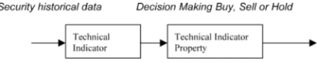
Fig. 1. Current process in technical analysis 0eld.
qualitative judgments are completely removed from the predictions.
We believe fuzzy logic systems are easier to compre-hend and modify [4]. Few fuzzy systems have been created to forecast market activities usingfundamental indicators [8,9,12,14,18–20]. Our proposal is to use technical indicators with fuzzy logic to create a fuzzy indicator that recommends sell, buy and hold position. This method avoids over-reliance on quantitative data. It consists of few inputs (e.g. rate of change (ROC), stochastic and support=resistance indicators), one out-put variable (e.g. level of con0dence to take a certain action), and a few fuzzy rules expressingthe relation-ships amongthe 0nancial indicators. Our plan can be summarized as follows:
• To map many di:erent 0nancial indicators into new inputs that can be “fuzzi0ed”. Use fundamental in-dicators with fuzzy logic to set up long-term invest-ment plans and use technical indicators with fuzzy logic to set up short-term investment plans.
• To create membership functions; to associate be-tween inputs and outputs via fuzzy rules.
• To translate the fuzzy output into a crisp trading recommendations.
Based on all of the above, we believe our proposed fuzzy logic system is very 5exible, modular and easy to comprehend.
3. Stock evaluation process
The process used in technical analysis 0eld is shown in Fig. 1. Analysts in this 0eld use wide varieties of indicators to analyze individual stock markets. Each indicator has properties and interpretation. Market in-dicators typically fall into three categories: monetary, sentiment, and momentum.
Monetary indicators concentrate on economic data such as interest rate. They give an indication of the economic environment in which businesses operate.
Fig. 2. Rate of change (ROC) momentum indicator.
These external forces directly a:ect a business’ prof-itability and share price.
Sentiment indicators focus on investor expectations. For a large market such as New York Stock Exchange, many sentiment indicators are available. These include the Put=Call ratio, the ratio of bullish versus bearish investment advisors, etc.
The third category of market indicators, momentum, shows what prices are actually doing. Examples of momentum indicators include the following:
1. The price=volume indicators applied to the various market indices.
2. The number of stocks that made new highs versus the number of stocks makingnew lows.
3. The relationship between number of stocks that ad-vanced in price versus the number that declined. 4. The comparison of the volume associated with
increased price with the volume associated with decreased price, etc.
Fig. 2 shows theROCmomentum indicator and its oversold and over bought properties. This indicator compares the price of today with the price ofxdays ago wherexrepresents the time period under consid-eration and limited tox¿2. Overbought and oversold lines are constructed on the basis of judgment [1].
Each of the indicators used in technical analysis has its limitation. The best result could be achieved when combiningmany indicators at the same time and evaluate their output collectively.
The new proposed process is shown in Fig. 3. This process consists of the following:
• Get historical dataR(nT)
Fig. 3. Proposed process for technical analysis. R(nT) represents the closingprice of a certain stock at samplenT.
• Develop technical indicators inputs →Ri(nT),
wherei= 1;2; : : : ; N.Ri(nT) represents the
techni-cal indicators used. For example R1(nT); R2(nT),
etc. could representROC, stochastic, etc. respec-tively.
• Develop a convergence module and create fuzzy logic inputs and input ranges →Yj(nT), where j= 1;2; : : : ; M. Yj(nT) represents the transformed
signal, which can be used in the fuzzy system.
• Develop a fuzzi0cation module and create member-ship functions for each input→jv(nT).
• Develop a fuzzy process and construct the rules that will govern system operation (knowledge base — fuzzy rules).
• Create fuzzy logic outputs and output ranges, de-termine how actions will be combined to form the executed action (decision stage).
• Evaluate outputs.
This process has many advantages. First, it pro-vides a new technique to handle the vagueness of the technical indicators. Second, it removes the complex-ity when many indicators are evaluated at the same time. Finally, it provides a systematic and standard-ized method to interpret information, information pro-cessing, decision making and actions.
4. Convergence module
This module maps the technical indicators into new inputs. These inputs are fed to the fuzzy system. This stage in the process is very important, it translates the indicator knowledge base information into di:erent type of signals that can be used in the fuzzy system. For example if the closingprice R(T) of a certain stock gets close to the support level (see Eq. (5)),
the system recommend a buy signal. To translate this knowledge into a fuzzy input, a new signal YSup is created (see Eq. (12)). This stage basically translates expert knowledge into fuzzy input signals.
Ri(T)→Yj(T); wherei= 1;2; : : : ; N;
j= 1;2; : : : ; M; M ¿N: (1) The number of the convergence module outputs (M) depends on the characteristics of the indicators used. Some indicators might not need any convergence and the mappingin this case is one to one. Other indicators might map into 2;3;or 4 signals.
M=Number of the convergence module output signals:
TheM signals generated by the convergence module are fed to the fuzzy logic system as inputs.
4.1. Inputs to the convergence module (technical indicators)
In this application, we will study the proposed pro-cess usingthree technical indicatorsN= 3. The fol-lowingwere chosen for this application:
• Rate of change momentum indicator
Rate of change (ROC) indicator is simply de0ned as the di:erence between the current price and the price at a speci0c time in the past. In this case we used 30 tradingdays as shown in Eq. (2).
ROC(nT) =R(nT)−R((n−30)T); n¿30;
where
R(nT) = security closingprice: (2)
• Stochastic momentum indicator
Stochastic indicator gives an indication of the stocks last closingprice relative to the stocks recent trading range.
The stochastic indicator has two main variables %K
and %D: %K(nT) = R(nT)−Rmin(nT) Rmax(nT)−Rmin(nT) 100; (3)
whereRmin(nT); Rmax(nT) are the minimum and
maximumR(nT) over a 30 day period, respectively. %D(nT) = n (n−3) %K(nT) 3 ; n¿3: (4)
• Support=resistance indicator.
Support=resistance indicator is computed by taking 2above and 2below the 30-day price average as shown in Eqs. (5) and (6). This indicator represents the dynamic support and resistance of the price [1]. Support level =Avg(nT)−2(nT); (5) Resistance level =Avg(nT) + 2(nT); (6) where
(nT) = n
n−30(R(nT)−Avg(nT))2
30 ;
Avg(nT) = 30 day price average =
n
n−30R(nT)
30 :
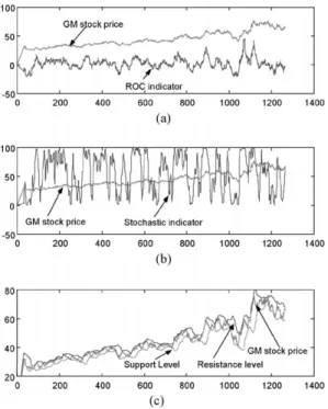
The three indicators used ROC, stochastic (%K), and support=resistance alongwith the security closing price are shown in Fig. 4.
4.2. Output of the convergence module (fuzzy logic inputs)
The N inputs discussed in the previous sec-tion were fed to the convergence module. In this speci0c example the convergence module resulted in seven signals M= 7. Fig. 5 shows the inputs and outputs of the convergence module. Where
YROC; YdROC=dt; Y%D; Y%K−%D; YSup; YRes and YAvg are
de0ned in Eqs. (7)–(13)
YROC(nT) = R(nTR)((−nR−((n30)−T30)) T)); n¿30;
(7) where
Fig. 4. Technical indicators: (a) ROC, (b) stochastic %K, (c) support and resistance levels.
Yd(ROC) dt(nT)
= YROC((n−2)T)−YROC(nT); n¿2; (8) Y%D(nT) = %D(nT); (9)
Fig. 5. Convergence module.
Y%D−%K(nT) =Y%D(nT)−Y%K(nT); where Y%K(nT) = %K(nT); (10) YRes(nT) =Avg(nT) + 2−R(nT); n¿30; (11) YSup(nT) =R(nT)−(Avg(nT)−2); n¿30; (12) YAvg(nT) =R(nT)−Avg(nT); n¿30: (13) 5. Fuzzi#cation module
This step in the process is designed to model peo-ple’s cognitive states. By analyzing each output of the convergence module, study its function and evaluate its e:ects with other signals, an indication for a future price movement starts to emerge. For example state-ments like:
IfY1(nT) is large, in another word if theROCindicator
is large, then the price is likely to move higher. IfY6(nT) is large, in another word if the price is close
to the resistance level, then the price is likely to move lower.
These statements lead to ambiguity and lack of 0rm-ness in decision making. Fuzzy logic technique has the ability to accommodate ambiguity by mixing multiple indicators to minimize ambiguity. The word
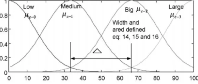
largeused in the example above “If ROC is large” is not well de0ned it is fuzzy.Largeis dependent on the value of what is beingmeasured. For example in Fig. 4(a), theROCranges from−20 to 50 while the resistance level ranges from−3 to 60. Due to the dif-ferences of input ranges for each of the fuzzy inputs, a value of say 40 may be consideredlargeforROC but may not be consideredlargefor resistance level. Fuzzy logic provides a mechanism to quantify such fuzzy concept. This is achieved by usingmembership grade function, which is a mapping from the domain of a fuzzy input value to a real value ranging from 0 to 1. This mappingrepresents the degree of membership to a class de0ned by the user for a given application. In the technical analysis 0eld application the classes we selected aresmall,medium,big and largeto rep-resent the four levels of quanti0cation of each input value range. The M signals de0ned in the previous section are mapped to the fuzzy space [0;1] usingthe bell shaped membership function, these bell shaped functions can be determined from either simple or so-phisticated elicitation procedures. The designer could start with simple set of membership functions and start re0ningthem by experimentingwith di:erent rules and membership functions. The bell shape distribution membership functions were adapted in this design. The bell shape membership function has the property of beingsmooth and nonzero at all points [11].
The membership functions used in this paper are derived usingEqs. (14)–(16) as shown below:
jv(nT) = exp −(Yjv(nT)−wjv)2 22 jv ; 06jv61; (14)
wherewjv andjvspecify the mean location and the
width of the bell shaped function, respectively.
jv= qj; (15) wjv=vj+Inf(Yj); v= 0; : : : ; l−1; (16)
where
j=Sup(Yjl)−−1Inf(Yj) for this equationl¿2;
wherelis the number of fuzzy bell shapes or quan-tization levels. Inf(Yj); Sup(Yj) are the dynamic
lower and upper bound of Yj; respectively. Inf(Yi)
and Sup(Yi) are calculated dynamically; as more
and more samples become available new Inf(Yi)and
Sup(Yi)emerges.q=proportionality constant.
Forv= 0:
wj0=Inf(Yi):
Forv=l−1
wj(l−1)= (l−1)j+Inf(Yj)
= (l−1)Sup(Yil)−−1Inf(Yi)+Inf(Yi)
=Sup(Yi);
wherejis the size of each partition when the fuzzy
inputYjis partitioned into equal regions.jv, the
stan-dard deviation of each bell shaped function and it is proportional to j, the proportionality constant q is
used to determine the spread of the bell shaped func-tions. In this application q is chosen as 2.35. This choice will be shown to produce a nicely distributed bell shaped function.
5.1. Application of the fuzzi9cation module
In this application, we chose l= 4. UsingEqs. (14)–(16) to calculate the mean and the width of the bell shaped membership functions for Y1(nT) is
shown:
w10 =Inf(Y1);
w11 =Sup(Y1)−3 Inf(Y1) +Inf(Y1); w12 = (2) Sup(Y1)−Inf(Y1) 3 +Inf(Y1); w13 =Sup(Y1); 10=11=12 =13= Sup(Y1)−Inf(Y1) 3(2:35) ; (17) where
Inf(Y1) = lower bound of Y1=YROC(nT);
Fig. 6. ROC fuzzy membership functions.
Fig. 7. Fuzzi0cation module.
Inf(Yi); Sup(Yi) are based on the previous sample
points:
Eq. (17) is plotted in Fig. 6.
Wherejvrepresents the strength of the fuzzy input Yj(nT) to the classvof the fuzzy inputYj(nT) where v=low; medium; big or large:
6. Fuzzy processing
Generally speaking, there are three main types of decisions: riskless choice, decision makingunder un-certainty, and risky choice. With this system, we are tryingto employ a decision makingunder uncertainty [22]. The distinction between risk and uncertainty hinges upon whether probabilities are known exactly or whether they must be judged by the decision-maker with some degree of imprecision. Decisions are made based on fuzzy rules (Fig. 7). These rules are characterized by a collection of fuzzy IF–THEN
Fig. 8. Output membership function.
rules in which the preconditions=post-conditions in-volve linguistic variables. This collection of fuzzy rules characterizes the behavior of the system in a linguistic form that is close to the way human think. After establishinga set of rules and membership functions that demonstrate feasibility, the designer can re0ne the system by experimentingwith di:erent rules and membership functions to achieve adequate results. The general form of the fuzzy rules in case of multi-input–single-output systems (MISO) is IFY1 isA1; : : : ;AND=ORYmisAmthenCisAL;
(18) where (Y1 is A1; : : : ;AND=ORYm isAm) are the
pre-conditions and C is the post-conditions, Y1 and Ym
are input variables, C is the output variable, A1 is
the class de0ned on Y1, Am is the class de0ned on Ym, andAL is class de0ned onC [7]. The antecedent
(the rule’s premise) describes to what degree the rule applies, while the conclusion (the rule’s consequent) assigns a membership function to the output vari-able. The output variable is assigned a range between Inf(C) = 0 and Sup(C) = 100. A low value repre-sents excellent opportunity to sell the stock and a high value represents excellent opportunity to buy the stock. Eqs. (14)–(16) were used to construct the out-put membership functions (low,medium,big,large) as shown in Fig. 8.
Let c−i denotes the fuzzy membership grade of
fuzzy outputC to the class i of fuzzy outputC. For example “Cis large” denotes the membership of the fuzzy output to the class large for the fuzzy output. Its output is computed usingthe membership grade functionc−3.
Mamdani’s fuzzy implication method is adopted in this paper. In this mode of reasoning, the strength
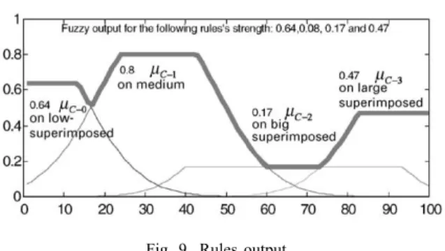
Fig. 9. Rules output.
of theith fuzzy rule is calculated by evaluatingthe strength of the preconditions i(degree of truth) then
superimpose it on the correspondingoutput member-ship [13]. The output membermember-ship function is clipped o: at a height corresponding to the rule premise’s computed degree of truth as described by Eq. (19).
C−i(w) = i∧c−i(w); (19)
wherewis the range of values that the rule conclusion can take,∧operator is de0ned as the min function [5].
i∧c−i(w) produces a output membership function C−i(w) clipped o: at a height equal to the i value
as shown below in Section 6.1, Fig. 9.
If the result due to rule 0 is recommendingan action
C−0(w) and the result due to rule 1 is recommending
an actionC−1(w), etc. Then accordingto Mamdani’s
method the overall result is
C(w) =C−0(w)∨C−1(w)∨ · · · ∨C−i
⇒C(w) = ( 0∧c−0(w))∨( 1∧c−1(w))
∨ · · · ∨( i∧c−i(w)); (20)
whereC(w) is a pointwise membership function for
the combined conclusion of rules 0;1;2; : : : ; i. The∨operator is de0ned as themaxfunction [5]. 6.1. Application of the fuzzy processing
Accordingto experts buy condition occurs ifROC is large, and the rate of change of ROC is highly changing and positive. A sell condition occurs ifROC is low and the rate of change of ROC is loosing momentum. If we use the classes de0ned above the
expert’s requirements to buy and sell can be summa-rized as follows:
• Buy ifYROC is bigandYdROC=dtis big.
• Sell ifYROC is low andYdROC=dt is medium.
Similarly for stochastic, the expert recommends a buy condition if %D is large (see Section 4:2:2). This statement can be translated in the fuzzy system as follows:
• Buy condition occurs ifY%Dis large.
• Sell condition occurs ifY%Dis low.
For the support=resistance indicator the expert buys if the price is far away from the resistance level or if it is close to the support level. This statement can be translated in the fuzzy system as follows:
• Buy ifYSup(nT) is low.
• Sell ifYRes(nT) is low.
Some of the requirements discussed above were used as a stand-alone fuzzy rule and some were joined with other indicators to make a more con0dent fuzzy rule see details in the followingsection.
Rule 0: IF {Y1(nT) is big and Y2(nT) is big} THEN C is large
Rule 1: IF {Y1(nT)is low and Y2(nT)is medium} THEN C is low
Rule 2: IF Y2(nT)is large THEN C is big
Rule 3: IF Y2(nT)is low THEN C is medium
Rule 4: IF Y7(nT)is large THEN C is large
Rule 5: IF Y4(nT)is large THEN C is big
Rule 6: IF {Y4(nT) is low and Y7(nT) is low} THEN C is low
Rule 7: IF Y3(nT)is large THEN C is big
Rule 8: IF {Y2(nT) is large and Y3(nT) is large} THEN C is large
Rule 9: IF {Y5(nT)is big and Y7(nT)is medium}
THEN C is medium
Rule 10: IF Y6(nT)is low THEN C is big.
As described in the above rules the number of fuzzy inputs is 7 (M= 7) and the number of de0ned classes over the output range are 4 {low;medium; big; and large}. The combined conclusion of rules can be de-0ned as follows:
Combined rule for class large:
IF {Y1(nT) is big and Y2(nT) is big} or {Y2(nT)is large andY3(nT)is large}orY7(nT) is large THEN Cis large.
Combined rule for class big:
IF Y2(nT) is large or Y6(nT) is large or Y3
(nT)is large orY5(nT)is low THEN Cis big
Combined rule for class medium:
IF {Y4(nT) is big or Y7 (nT) is medium or Y2(nT)is low}THEN Cis medium
Combined rule for class low:
IF {Y1(nT) is low and Y2(nT) is medium} or{Y6(nT)is low andY7(nT)is low}THENC is low.
Letjvdenote the fuzzy membership grade of fuzzy
inputYj(nT) to the classvof fuzzy inputYj(nT). For
exampleY2(nT)is bigdenotes the membership of the
fuzzy input 2 to the class bigfor fuzzy input 2. Its value is computed usingthe membership grade function23.
Similarly,Y1(nT)is lowis computed by11, etc. The
antecedent of rule 0 is covered as follows:
The value of the antecedent of rule 0IF{Y1(nT)is low and Y2(nT)is medium}or {Y6(nT) is low and Y7(nT)is low}THEN Cis lowis denoted as 0
0={11and22}or {61 and71}
=max{min(22; 11); min(61; 71)};
where the “and”, “or” operators are replaced by min, max operator, respectively.
Since each of the membership grade function value ranges between 0 and 1. The value of the antecedent for each combined rule{ i; i= 0;1;2;3}also ranges
between 0 and 1.
Mamdani’s fuzzy implication method is used to combine the rules and calculate the output. As de-scribed in Eqs. (19) and (20) theith combined fuzzy rule is calculated by evaluatingthe strength of the pre-conditions i(degree of truth) then superimpose it on
the correspondingoutput membership c−i(w). The
followingmembership strengths will result:
C−0(w) = 0∧c−0(w)
= Result of the “combined rule for low”: C−1(w) = 1∧c−1(w)
= Result of the “combined rule for medium”:
C−2(w) = 2∧c−2(w)
= Result of the “combined rule for big”: C−3(w) = 3∧c−3(w)
= Result of the ”combined rule for large”;
where
0=max{min(11; 22);min(61; 71)} 1=max{21;min(43; 72)}
2=max{24; 64; 34; 51}
3=max{min(23; 13);min(23; 34); 74} c−0(w); c−1(w); c−2(w), and c−3(w) are the
fuzzy membership correspondingtolow,medium,big and large,respectively.
Mamdani’s process then produces
C(w) =C−0(w)∨C−1(w)∨ · · · ∨C−3
= ( 0∧c−0)∨( 1∧c−1)∨( 2∧c−2)
∨( 3∧c−3):
For example if the strengths of the rules 0–3 are 0.64, 0.8, 0.17, and 0.47, respectively. The result of this op-eration as described in Mamdani’s paper is a mem-bership functionC(w) as shown by the solid line in
Fig. 9, whereC(w) is a pointwise membership
func-tion for the combined conclusion of all rules. This function has to be translated (defuzzi0ed) to single value as discussed next.
7. Defuzzi#cation
Defuzzi0cation is a mappingprocess from a fuzzy space de0ned over an output universe of discourse into a nonfuzzy (crisp) action. The method adopted in this paper is center of area (COA) [6]
F(nT) = L i C(Zi)(Zi) L i C(Zi) ; (21)
whereLrepresents the number of quantization levels of the outputC; Ziis the amount of control output at
the quantization leveli; C(Zi) represents the
mem-bership value in the output fuzzy set.
This calculation implies that for a speci0cR(nT) in-put, a fuzzy valueF(nT) will be created. WhenF(nT) is close to the 100 (high end), the stock is a strong buy. On the other hand whenF(nT) is close to 0 (low end), the stock is a strongsell.
8. Systemevaluation
Any investment always involves a tradeo: between risk and reward. The higher the reward an investor seeks, the greater the risks and uncertainties are likely to be. Over any given period, stock prices will 5uctu-ate widely in response to company news, changes in industry conditions, the overall economics and poten-tial climate, unexpected events, and shifts in investor psychology [2]. In our paper, we presented the risk factor as a function of the trigger buy or sell level of the fuzzy indicator.
Three years of stock price data of di:erent com-panies have been fed to this system for evaluation. Companies with high performance, very low perfor-mance and average perforperfor-mance were tried. The re-sults were excellent and it proved the 5exibility of the system.
The proposed fuzzy logic system was used on the followingcompanies:
1. Western Digital Corp. (WDC) 2. Intel Corp. (INTC)
3. Compaq Computer Corp. (CPQ) 4. General Motors Corp. (GM)
These companies performed di:erently over the years. Di:erent strategies can be implemented using the fuzzy indicator. Two strategies are shown:
8.1. First strategy — identify triggers based on system performance
Every X tradingdays the system calculates new trigger levels based on the system performance. The trigger levels will be used in the nextX tradingdays. WhereX can be any number and it depends on the followingmain issues:
1. Investor risk.
2. Stock’s price long-term trend. 3. Volatility of the stock.
In this application we choseX to be 30. This strategy requires evaluatingall di:erent possible combinations of trigger levels applied to the data of the previous period. The system then uses the best performance set of trigger levels in the next period of trading to recommend sell and buy states.
Strategy description. At the end of each period the system uses the previous period data to check for certain conditions and propose certain actions as de-scribed in the followingprocedure:
• IfF(nT)¿UTLandM2= 0 then a stock buy con-dition occurs. This results in the followingactions:
Q=M2=SP;
Gain=Q∗SP−M1: (22)
• IfF(nT)6LTLandM2 = 0 then a stock sale con-dition occurs. This results in the followingactions:
M2 =Q∗SP;
Gain=M2−M1; (23) whereUTLis the upper trigger level,LTLthe lower trigger level,M1 the money invested at the beginning of the period,M2 the accumulated money at the end of the period,Qthe number of shares owned andSP
the stock price.
The proposed strategy executes the above proce-dure and calculates theGainfor every possible com-bination ofUTLandLTLusingthe data collected in the previous period. The limits ofUTLandLTLare de0ned as follows:
516UTL6100 and 06LTL649:
The combination ofUTLandLTLthat results in max-imumGainwill be used for the next period.
8.2. Second strategy — identify triggers based on risk
This strategy calls forUTLandLTLto be constant. The level will be chosen as a function of the investor risk taking. If the investor is not willing to take risk
the range betweenUTLandLTLis very small. For exampleUTL= 51 andLTL= 49. If the Investor is a risk taker then the range between UTL andLTLis big. For exampleUTL= 60 andLTL= 40.
These strategies were implemented and shown in the following0gures.
9. Systemresults and data
The followingstrategies were applied to each company (the chosen companies are described in Section 8).
1. 1st strategy usingUTL= 51 andLTL= 49 simulat-inglow risk investor.
2. 1st strategy usingUTL= 60 andLTL= 40 simulat-inghigh risk investor.
3. 2nd strategy.
In each case, the system will take an initial investment of $10;000 and calculates the return and total pro0t. The transaction cost is assumed to be $10=transaction. Total net pro0t already included the transaction cost in the calculation.
Total net pro9t
=Final price(share value∗No:of shares)
−Initial invest−Transaction cost: (24) Note: Tax implications are not included in the cal-culation.
9.1. Evaluation of Western Digital stock price movement (WDC)
Western Digital stock price movement from August-28-1995 until August-27-1999 went through a cycle that consisted of an up trend followed by a downtrend period. The system was evaluated during the uptrend from August-28-95 until September-5-1997 and then duringthe downtrend period from September-5-1997 until August-27-99. Sections 9.1.1 and 9.1.2 detail the results usingthe three proposed strategies described in Section 9.
9.1.1. Evaluation of WDC uptrend stock price movement
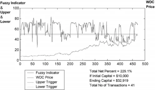
• WDC evaluation using the1st strategy(low risk investment proposal UTL= 51 and LTL= 49): Western Digital Corporation stock price was rising from September 5th 1995 until August 27th 1999. The price went up from $8 per share to $50 per share in 500 days of trading. For a low risk in-vestment strategy, the return was 229.1% and the number of transactions was 41. If $10;000 were in-vested in this stock on August 28th 1995 and kept until September 5th 1999, the investor would have a net worth value of $32;919. Details are shown in Fig. 10.
• WDC evaluation using the1st strategy(high-risk investment proposal UTL= 60 and LTL= 40): As expected, the high-risk investment strategy yielded higher return in an uptrend market. The initial $10;000 resulted in $43;200 compared to the $32;919 calculated for a low risk investor. The number of transactions was lower because risky investor can tolerate more volatility. Details are shown in Fig. 11.
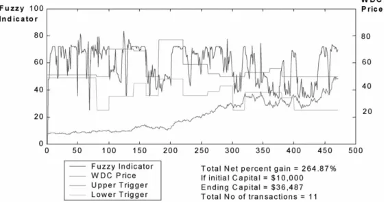
• WDC evaluation using the2nd strategy proposal (UTL and LTL are functions of system perfor-mance): This strategy evaluates the trigger levels based on the previous period. The total net pro0t was 264.87% and the total number of transactions was 11. If $10;000 was invested in this stock on August 28th 1995 and kept until September 5th 1999, the investor would have a net worth value of $36;487. Details are shown in Fig. 12.
9.1.2. Evaluation of WDC down trend stock price movement
• WDC evaluation using the1st strategy (low-risk investment proposal UTL= 51 and LTL= 49): Western Digital Corporation stock price was drop-pingsharply from September 5th 1995 through August 27th 1999. The price went down from $58 per share to $5 per share in 500 tradingdays. If $10;000 were invested in this stock on September 5th 1999 and kept until August 27th 1999, the in-vestor would have a net worth value of $862. This implies that the total net loss would be 91.38%. If the investor used the low risk strategy ofUTL= 51
Fig. 10. WDC 1st strategy low risk (uptrend).
Fig. 11. WDC 1st strategy high risk (uptrend).
andLTL= 49, the total net loss would be 29.47% compared to 91.38%. This means a $10;000 in-vested on September 5th 1999 would result in a net value of $7053 on August 27th 1999. Details are shown in Fig. 13.
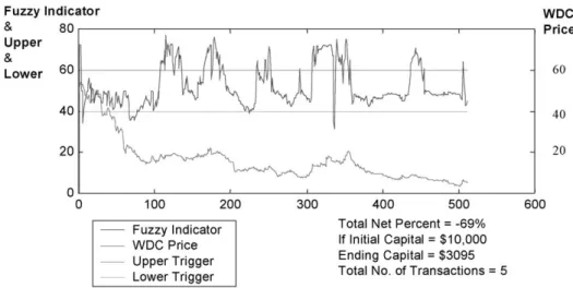
• WDC evaluation using the1st strategy(high-risk investment proposalUTL= 60andLTL= 40): As expected, the high-risk investment strategy lost more money in a downtrend market. If $10;000 were invested in the stock on September 5th 1999
and kept until August 27th 1999, the investor would have lost 91.38%. If the investor used the high risk proposed strategy ofUTL= 60 and LTL= 40, the total net loss would be 69%. Details are shown in Fig. 14.
• WDC evaluation using the2nd strategy proposal (UTL and LTL are functions of system perfor-mance): This strategy evaluates the trigger levels based on the previous period. Usingthe fuzzy indi-cator, the total net loss was 36% compared to 91%
Fig. 12. WDC 2nd strategy (uptrend).
Fig. 13. WDC 1st strategy low risk (down trend).
loss without the fuzzy indicator. Details are shown in Fig. 15.
9.2. Evaluation of INTEL corporation stock price movement (INTC)
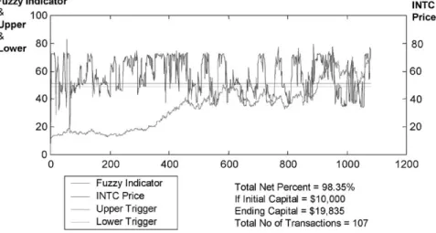
• INTEL stock evaluation using the 1st strat-egy (low risk investment proposal UTL= 51 and
LTL= 49): Intel stock prices from January 3rd 1995 through July 30th 1999 were collected and fed into the fuzzy system model. Duringthis pe-riod the stock was rising. For the low investment strategy the return was 98.35%. If $10;000 were invested in this stock on January 3rd 1999 and kept until July 30th 1999, the investor would have a net worth value of $19,835 and the total number
Fig. 14. WDC 1st strategy high risk (down trend).
Fig. 15. WDC 2nd strategy (down trend).
of transactions would be 107. Details are shown in Fig. 16.
• INTEL stock evaluation using the 1st strategy (high-risk investment proposal UTL= 60 and
LTL= 40): As expected, the high-risk investment strategy yielded higher return in an uptrend envi-ronment. The initial investment of $10,000 resulted in $25,632 compared to $19,835 calculated for a low risk investment strategy as shown in Fig. 17. The number of transactions was lower because
risky investor can tolerate more volatility and therefore fewer transactions.
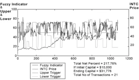
• INTEL stock evaluation using the 2nd strategy proposal(UTL and LTL are functions of system performance): This strategy evaluates the trig-ger levels based on the previous period. The total net pro0t was 217.76%. If $10,000 were invested in this stock on January 3rd 1999 and kept un-til July 30th 1999, the investor would have a net worth value of $31,776 and the total number of
Fig. 16. INTEL 1st strategy low risk.
Fig. 17. INTEL 1st strategy high risk.
transactions would be 21. Details are shown in Fig. 18.
9.3. System evaluation of compaq computer stock price movement (CPQ)
• Compacq computer stock evaluation using the1st strategy (low-risk investment proposalUTL= 51 and LTL= 49): Compacq Computer stock prices from January 3rd 1995 until July 30th 1999 were collected and fed into the fuzzy system model. For the low investor strategy the return was 147%. If
$10,000 were invested in this stock on January 3rd 1999 and kept until July 30th 1999, the investor would have a net worth value of $24,709 and the total number of transactions would be 78. Details are shown in Fig. 19.
• Compacq computer stock evaluation using the1st strategy(high-risk investment proposalUTL= 60 and LTL= 40): The high-risk investment strategy yielded a higher return in an uptrend environment. The initial $10,000 resulted in $33,916 compared to $24,709 calculated for a low risk investment strat-egy. The number of transactions was also lower
Fig. 18. INTEL 2nd strategy.
Fig. 19. CPQ 1st strategy low risk.
because risky investor can tolerate more volatility. Details are shown in Fig. 20.
• Compacq computer stock evaluation using the2nd strategy proposal(UTL and LTL are functions of system performance): This strategy evaluates the trigger levels based on the previous period. The total net pro0t was 87%. If $10,000 were invested in this stock on January 3rd 1999 and kept until July 30th 1999, the investor would have a net worth value of $18,766 and the total number of transactions would be 22. Details are shown in Fig. 21.
9.4. System evaluation of General Motor corporation stock movement (GM)
• General Motor stock evaluation using the1st strat-egy (low-risk investment proposal UTL= 51 and
LTL= 49): General Motor stock prices from Jan-uary 3rd 1995 until May 10th 1999 were collected and fed into the fuzzy model. Usingthe low invest-ment strategy the return was 58.12%. If $10,000 were invested in this stock on January 3rd 1999 and kept until May 10th 1999, the investor would have
Fig. 20. CPQ 1st strategy high risk.
Fig. 21. CPQ 2nd strategy.
a net worth value of $15,813 and the total number of transactions would be 124. Details are shown in Fig. 22.
• General Motor stock evaluation using the 1st strategy(high-risk investment proposalUTL= 60 and LTL= 40): The high-risk investment strategy yielded higher return in an uptrend environment.
In this case the uptrend is not steep enough and therefore takingmore risk did not yield a much higher gain. The initial $10,000 resulted in $17,081 compared to $15,813 calculated for a low risk investment strategy. The number of transactions was lower because risky investor can tolerate more volatility. Details are shown in Fig. 23.
Fig. 22. GM 1st strategy low risk.
Fig. 23. GM 1st strategy high risk.
• General Motor stock evaluation using the 2nd strategy proposal (UTL and LTL are functions of system performance): This strategy evaluates the trigger levels based on the previous period. The total net pro0t due to this strategy was 71%. If $10,000 were invested in this stock on January 3rd 1999 and kept until May 10th 1999, the investor would have a net worth value of $17,101 and the total number of transactions would be 45. Details are shown in Fig. 24.
10. Conclusion
This paper examined fuzzy logic systems in the 0-nance arena. It simulated human behavior in reacting to stock price movement and formation. A number of inputs were created to recommend buy=sell of a spe-ci0c stock when certain price formation exists. We simpli0ed some details on investingprocedures (cost per transaction is constant, taxation e:ects, etc.) in order to highlight the properties of the methodology
Fig. 24. GM 2nd strategy low risk.
presented. This simulation system used Matlab pro-gram to generate the results.
In this study, we applied fuzzy informational tech-nologies to investments through technical analysis. Most investment models are of a proprietary nature and their characteristics are not reported in the schol-arly literature. Pruitt and White [16] is a published as-sessment of the potential of technical analysis. They used three technical indicators (cumulative volume, relative strength, and moving average) to build their tradingmodel. Our system examined various compa-nies and proved to be e:ective. The investment returns were excellent. Most companies consider the perfor-mance of S&P 500 as average perforperfor-mance. Our re-sults surpassed the S&P 500 by a substantial amount. The buy and sell trigger level can produce di:erent re-sults. Accordingto our analysis, the decision to choose the trigger levels for sell and buy depends on the in-vestor and the stock’s long-term trend. Because of this, di:erent strategies can be implemented using the fuzzy indicator to match the investor preferences and the industry conditions. One strategy was described and implemented. The results were excellent as shown in Section 8.
References
[1] S.B. Achelis, Technical Analysis from A to Z, New York, 1993.
[2] B. Apostolou, N. Apostolou, Keys to Investingin Common Stocks, 1995.
[3] M.E. Azo:, Neural Network Time Series Forecastingof Financial Markets, Wiley, New York, 1994.
[4] D. Benachenhou, Smart tradingwith FRET, TradingOn The Edge, Wiley, New York, 1996.
[5] H.R. Berenji, Fuzzy logic controllers, in: R. Yager, Lot0 (Eds.), An Introduction to Fuzzy Application in Intelligent Systems, Zadeh, Norwell, 1992, pp. 69–89.
[6] M. Braae, D.A. Rutherford, Theoretical and linguistic aspects of the fuzzy logic controller, Automatica 5 (1979) 553–577. [7] Chin-TengLin, G. Lee, Neural Fuzzy Systems, Upper Saddle
River, 1996.
[8] G.J. Deboeck, TradingOn The Edge, Wiley, New York, 1996. [9] J.C. Francis, Management of Investment, 3rd Edition,
McGraw-Hill Inc., New York, 1993.
[10] E. Gately, Neural Networks for Financial Forecasting, Wiley, New York, 1996.
[11] A. Kaufmann, M. Gupta, Introduction to Fuzzy Arithmetic, New York, 1995.
[12] K.P. Lam, Chiu-KC, Chan-WG, Neural network in 0nancial engineering, in: An Embedde Fuzzy Knowledge Base for Technical Analysis of Stocks, World Scienti0c Publishing Co., Singapore, 1996.
[13] E.H. Mamdani, S. Assilian, An experiment in linguistic synthesis with a fuzzy logic controller, Internat. J. Mach. Studies 1 (1975) 1–13.
[14] O’Neil, J. William, How to Make Money in Stocks, 2nd Edition, McGraw-Hill Inc., New York, NY, 1995. [15] M.J. Pring, Technical Analysis, New York, 1991.
[16] Pruitt, White, The CRISMA tradingsystem: who says technical analysis can’t beat the market, J. Portfolio Management (1988) 55–58.
[17] A.N. Refenes, N. Burgess, Y. Bentz, Neural networks in 0nancial engineering: a study in methodology, IEEE Trans. Neural Networks 8 (6) (1997) 1222–1267.
[18] R. Simutis, Fuzzy logic based stock trading system, Proc. IEEE=IAFE Conf. on Computational Intelligent of Financial Engineering, New York, 2000.
[19] S. Singh, J. Fieldsend, Financial time series using fuzzy and longmemory pattern recognition systems, Proc. IEEE=IAFE Conf. on Computational Intelligent of Financial Engineering, New York, 2000.
[20] Ta-Chung-Chu, Chung-Tsen-Tsao, Yeou-Ren-Shiue, Application of fuzzy multiple attribute decision makingon company analysis for stock selection, 1996 Proc. of the 1996 Asian Fuzzy Systems Symposium, IEEE, New York, NY, USA, 1996, pp. 509–514.
[21] R.R. Trippi, E. Turban (Ed.), Neural Network in Finance and Investing, Probus Publishing Company, 1993.
[22] J.F. Yates, Judgment and Decision Making, Prentice-Hall, Englewood Cli:s, NJ, 1990.