Robust Ranking Models via Risk-Sensitive Optimization

(1)

Robust Ranking Models via Risk-Sensitive Optimization

Lidan Wang

Dept. of Computer Science

University of Maryland College Park, MD

Paul N. Bennett

Microsoft Research One Microsoft Way

Redmond, USA

Kevyn Collins-Thompson

Microsoft Research

One Microsoft Way Redmond, USA

ABSTRACT

Many techniques for improving search result quality have been proposed. Typically, these techniques increase average effectiveness by devising advanced ranking features and/or by developing sophisticated learning to rank algorithms. How-ever, while these approaches typically improve average per-formance of search results relative to simple baselines, they often ignore the important issue of robustness. That is, al-though achieving an average gain overall, the new models often hurt performance on many queries. This limits their application in real-world retrieval scenarios. Given that ro-bustness is an important measure that can negatively impact user satisfaction, we present a unified framework for jointly optimizing effectiveness and robustness. We propose an ob-jective that captures the tradeoff between these two com-peting measures and demonstrate how we can jointly opti-mize for these two measures in a principled learning frame-work. Experiments indicate that ranking models learned this way significantly decreased the worst ranking failures while maintaining strong average effectiveness on par with current state-of-the-art models.

Categories and Subject Descriptors

H.3.3 [Information Retrieval]: Retrieval Models

Keywords

Re-ranking, robust algorithms, machine learning

1. INTRODUCTION

Many approaches for learning highly effective ranking mod-els for search have been proposed in recent years [19, 5, 25]. Most commonly, they apply well-developed machine learning algorithms to construct ranking models from training data by optimizing a given IR metric. While the learned rank-ing models can be highly effective, these approaches have mostly ignored the important issue of robustness – in addi-tion to performing well on average, the model should, with

Permission to make digital or hard copies of all or part of this work for personal or classroom use is granted without fee provided that copies are not made or distributed for profit or commercial advantage and that copies bear this notice and the full citation on the first page. To copy otherwise, to republish, to post on servers or to redistribute to lists, requires prior specific permission and/or a fee.

SIGIR’12,August 12–16, 2012, Portland, Oregon, USA.

high probability, not perform very poorly for any individ-ual query. Often effectiveness and robustness are competing forces that counteract each other: models optimized for ef-fectiveness alone may not meet the strict robustness require-ment for individual queries.

This paper introduces learning robust ranking models for search via risk-sensitive optimization, by exploiting and op-timizing the tradeoffs between model effectiveness and ro-bustness. At a basic level, this framework learns ranking models whose effectiveness and robustness can be explic-itly controlled. While effectiveness and robustness can be thought of in terms of absolute performance, one can spe-cialize these concepts to a case where we desire to perform well relative to a particular baseline – for example a person-alized system vs. the non-personperson-alized baseline, query ex-pansion vs. no exex-pansion, or a learned model vs. a retrieval formula. In this case, we can specialize the notions of ef-fectiveness and robustness to say that we wish to have high average gain relative to the baseline (i.e., positive change in performance) while at the say time incurring low risk rela-tive to the baseline (i.e., low probability of performing worse than the baseline for any particular query).

We develop a unified learning to rank framework for jointly optimizing both gain and risk by introducing a novel trade-off metric that decomposes gain into reward (upside) and risk (downside) relative to a baseline. While this objective could be integrated into many learning models, we show how to extend and generalize a state-of-the-art algorithm Lamb-daMart [6] to optimize the new objective. We empirically demonstrate that models learned this way outperform both a selective personalization approach and standard learning to rank models in terms of achieving an optimal balance between gain and risk. Moreover, our results also provide important insights into why our learned models are more ro-bust in terms of the learning convergence property of the new model as compared to standard effectiveness-centric models.

2. RELATED WORK

Multi-objective learning to rank has received much atten-tion in recent years [31, 13]. This is because, in many prac-tical settings, the performance of a ranking model is eval-uated by multiple measures of interest (e.g., NDCG, MAP, freshness, efficiency). Multi-objective learning to rank trains ranking models to simultaneously optimize multiple IR mea-sures. Svoreet al. [31] use a standard web relevance mea-sure, NDCG, as the primary optimization metric and a rele-vance derived from click-data is used as the secondary met-ric; the performance of the primary measure is maintained

(2)

constant while the algorithm tries to improve the secondary measure. Daiet al.[13] develop a multi-objective learning to rank algorithm for freshness and relevance by extending a state-of-the-art divide and conquer ranking approach [3]. The key differences between these and our work is that we treat both risk and reward, which are potentially competing measures, as first-class metrics during optimization, unlike the “tiered” approach [31]; however, more importantly, our risk measure is inherently different from the previous multi-objective learning to rank metrics – instead of capturing just another facet of web search [31, 13], risk evaluates the fitness of the ranking modelwith respect toa baseline model under a specific metric. In other words, risk is orthogonal to the previous multi-objective metrics – risk is defined on top of these metrics with respect to a baseline model.

Although other risk-aware algorithms have been proposed for ad-hoc retrieval [35, 39] and query expansion [26, 10], our problem differs from them in three important dimen-sions. First, we focus on designing new learning to rank algorithms to create robust state-of-the-art ranking mod-els using boosted regression trees, rather than focusing on risk-minimization for language models or simple term-based models [35, 39, 34]. Second, unlike [10, 26], the source of risk in our setting comes from the fact that users and queries are diverse, so that a single model cannot serve all users or queries well. Thus we design a new risk-sensitive algorithm that effectively leverages query-dependent features to build models that are highly robust and effective for individual queries. Finally, these previous problems represent partic-ular strategies for ranking, hence their solutions cannot be trivially extended to the more general problem of learning robust ranking models for large-scale retrieval.

Risk can be indirectly addressed by building query-dependent models to better adapt to individual queries. This line of work resulted in recent papers that consider query-specific loss functions [4], where queries of different types (e.g., navi-gational, information) are optimized with different loss func-tions. Genget al.[18] proposed a k-Nearest Neighbor based method which trains a query-dependent ranking function for each query based on its nearest neighbors in the train-ing set. Bianet al. [3] proposed a clustering-based divide-and-conquer approach for building query-dependent rank-ing models. However, it is important to note that query-dependent models arenot perfect – just like any other mod-els, query-dependent models incur risk (e.g., reduced perfor-mance for some queries and gains for other queries), and this fact has been largely ignored as well. In a sense, our pro-posed framework generalizes and complements this thread of work by learning risk-sensitive query-dependent models.

There has been a great deal of research devoted to de-veloping effective retrieval models that have high average retrieval quality. This has given rise to a steady stream of techniques for effective ranked retrieval. Examples in-clude learning to rank [19, 5, 25], learning to re-rank [22], numerous term proximity models [27, 8, 32], and search per-sonalization [1, 36, 11]. However, unlike our work, they ig-nore the important issue of model robustness – while many queries see performance improvements, other queries are of-ten hurt by the new and complex models as compared to simple alternatives such as BM25 [29] and language models for information retrieval [28].

Our work also has connections to query difficulty and per-formance prediction for Web search [38], as well as selective

personalization [33]. These techniques mitigate risk in re-ranking by using a query performance prediction method to selectively re-rank queries whose baseline effectiveness is expected to be low, and avoid re-ranking for queries where the baseline effectiveness is already high. We note these techniques are robustness-centric, which may lead to overly reduced effectiveness due to unreliable decision in applying the model. In Section 5 we compare our approach to the use of selective re-ranking using performance variables.

It seems reasonable to assume that users tend to remem-ber the singular, spectacular failures of a search engine rather than the many successful searches that preceded them. How-ever, we are not aware of many user studies that have looked at the effect of IR robustness (or the lack thereof) on users’ perceptions of system quality. One exception is a recent user study of recommender systems [23] that showed how opti-mizing the accuracy of a system is not enough: among other interesting findings, they found that high-variance recom-mendation algorithms can create a bad user experience. In-formally, significant errors can have a large negative impact on the perceived quality of the system, even if the system frequently does well.

Finally, the termrobust ranking has been used previously in the literature, but with somewhat different meaning. For example, Li et al. [24] call ranking functions ‘robust’ that account for volatility in ranker scores, and thus, document ordering, over time, by taking into account the distribution of ranking scores over results. Others have used ‘robust ranking’ to refer to ranking algorithms that are less vulner-able to spam or noise in the training data [2].

3. MOTIVATION

Before proceeding, it is important to identify sources of uncertainty that contribute to low robustness in ranking models. In most search settings and especially Web search, both users and information needs are highly diverse, thus, it is unlikely a common set of ranking features and the same model learned from these features can optimally work for all users and queries. For instance, it has been shown that: queries with low click entropies typically will not benefit from search personalization [1, 36, 11]; queries with low query clarity will not benefit from query expansion tech-niques as much [16]. Ignoring these facts during model train-ing leads to a highly risky model. Although previous work has studied whether and when a learned model should be applied to a given query based on the aforementioned query-specific meta-features [33], the average effectiveness that re-sults from the robust application of the ranking model is generally ignored – which means the robustness is typically improved but at an overly aggressive cost in reduced av-erage effectiveness. We take a principled learning to rank approach that directly optimizes multiple requirements.

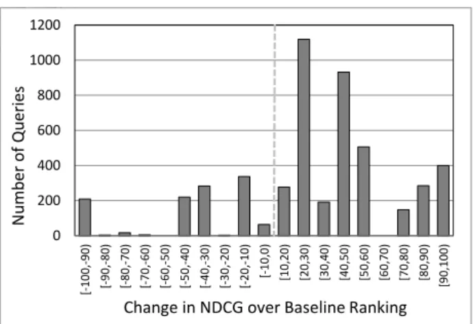
For instance, Figure 1 illustrates the improvements and degradations of a proposed model (tuned for average effec-tiveness) with respect to a baseline ranking across queries. The plots shows a high variance of the new results – the per-formance of a number of queries is improved (right side) at the expense of degraded results for other queries (left side). Directly optimizing for variance is a challenging task – vari-ance is inherently a set-based measure defined on the distri-bution of results quality over queries, but typically, learning to rank algorithms are not directly applicable to optimizing

(3)

0 200 400 600 800 1000 1200 [-10 0,-90 ) [-90 ,-80 ) [-80 ,-70 ) [-70 ,-60 ) [-60 ,-50) [-50 ,-40) [-40 ,-30) [-30 ,-20 ) [-20 ,-10 ) [-10 ,0 ) [10 ,20) [20 ,30) [30,40) [40,50) [50,60) [60 ,70) [70 ,80) [80 ,90) [90 ,100 ) N u m b er of Qu eries

Change in NDCG over Baseline Ranking

Figure 1: Typical helped-hurt histogram of re-ranking gains and losses compared to a given baseline ranking.

set-based measures. We instead adopt a simple approach suggested by this figure.

Informally, when compared to an alternative or baseline ranking, the probability of decreasing performance is related to the mass on the left-hand side of the figure. In fact the expectation of the left-hand side, which we call risk, is the amount we can expect to decrease retrieval quality on av-erage if we pick a query at random. Likewise, the expec-tation of the right-hand side, which we call reward, is the amount we can expect to improve retrieval quality on aver-age. By defining each average relative to the total number of queries rather than dividing reward by the number of improved queries and risk by the number of hurt queries, we control for issues of coverage. Typical methods optimize overall performance,Reward−Risk+Baseline, but since the baseline is fixed from the optimization point of view, this is equivalent to optimizing the difference,Reward−Risk. In order to control the risk or probability of harm, this suggests introducing a weight on the risk term that is user tunable. This is precisely what we do. In the next section, we for-malize this intuition before demonstrating how to optimize the objective in practice.

4. A LEARNING TO RANK APPROACH

FOR CREATING ROBUST MODELS

4.1 Problem setting

In this section, we present the formal setup for learning robust ranking models for Web search. Given a baseline rankingMbwe would like to construct a new ranking model

Mm with high average effectiveness across queries, without

degrading the performance of individual queries too much with respect to Mb. The exact instantiation of the

base-line Mb depends on the specific application of our general

framework. For personalization, Mb might be the initial

non-personalized ranking (e.g., optimized for the average user). In a production environment, Mb might represent

the results from an earlier release of the ranker. In learning to rank, Mb might be simpler models such as BM25 that

are known to be effective on a particular subset of queries. Our framework is applicable to these and any other ranking-based applications where a risk/reward tradeoff may exist.

4.2 Measuring risk and reward

One way to measure risk is by measuring the variance of the new ranking model with respect to baseline results. We instead adopt a variant of this approach, by introducing a risk functionFRISK(QT, Mb) to capture characteristics of

the variance with respect to model Mb over a training set

QT. We are interested in the downside risk of the new model,

defined as the average reduction in effectiveness due to using the new modelMmcompared to the baseline modelMb1.

FRISK(QT, Mb) = 1 N X Q∈QT max [0, Mb(Q)−Mm(Q)] (1)

whereNdenotes the total number of queries in the training set QT, and Mb(Q) and Mm(Q) denote the effectiveness

of the baseline model and new model for a given queryQ, respectively. We note that effectiveness can be measured by any commonly-used IR metrics (e.g. precision@k, recall, average precision, and NDCG@k). Thus, the downside risk accounts for the negative aspect of the retrieval performance across queries.

Similarly we defined reward in relative terms as the pos-itive improvement in effectiveness over baseline model Mb,

averaged across all queries in a training setQT:

FREWARD(QT, Mb) = 1 N X Q∈QT max [0, Mm(Q)−Mb(Q)] (2)

where notations N, Mb, and Mm are defined as before.

Thus, the reward function accounts for the positive aspects of the retrieval performance across queries. For any arbi-trary baseline,Mb, the overall gain for training setQT can

then be written:

FGAIN(QT) =FREWARD(QT, Mb)−FRISK(QT, Mb). (3)

Our goal is to automatically learn ranking models that better adapt to individual queries by optimally trading off between risk and reward. However, before we can learn such a well-balanced model, we must define a new metric that captures the tradeoff. Our objective function, which we call Risk-Reward tradeoffT, is defined as a weighted linear com-bination of gain (which includes risk and reward) and risk:

Tα(QT, Mb) = FGAIN(QT)−α·FRISK(QT, Mb) (4)

=FREWARD(QT, Mb)−(1 +α)·FRISK(QT, Mb)

where α ≥ 0 is a keyrisk-sensitivity parameter that con-trols the tradeoff between risk and reward. We chose this formulation so that the caseα= 0 corresponds to the stan-dard learning-to-rank objective to maximize averageFGAIN alone. Note thatT is not a single measure, but a family of measures, parameterized by the tradeoff parameter α. By varying α we can capture a full spectrum of risk/reward tradeoffs: from α= 0 (standard default ranking) to larger values ofαthat lead to lower-risk models, or small values of

αthat lead to higher gain models.

The most common approach to optimizing multiple objec-tives [30] is to linearly combine objecobjec-tives, as we have done with the risk and reward functions. While many other ways for combining metrics exist, such as by multiplication, divi-sion, geometric or harmonic means, optimizing an arbitrary

1

For simplicity of notation, in the remaining of the paperMb

will refer to both the baseline model and the effectiveness of the baseline model. A similar convention is used forMm.

(4)

optimization objective can be problematic in many learning algorithms. In contrast, linearly combined objectives are of-ten easily optimized. For our purposes, we will exof-tend the objective of the LambdaMart algorithm [37]. In Sec. 4.3, we prove that our tradeoff measureT satisfies a desirable consistency property [6].

4.3 Constructing robust ranking models

In this section, we describe how to learn models that di-rectly optimize the proposed tradeoff metricTα in the

pre-vious section. The basic assumption is that queries are dif-ferent, thus requiring potentially different ranking functions to be individually effective. Previous query-dependent mod-els [4, 18, 3] ignore risk. We devise learning to rank algo-rithms that directly optimize the tradeoff metric in the con-text of LambdaMart boosted regression trees framework [37].

4.3.1 Model and optimization algorithm

We choose to extend LambdaMart [37] for our ranking model. Boosted regression trees have been shown to be one of the best learning to rank models. In the recent Yahoo! Learning to Rank Challenge [9], boosting (and ensemble methods) have been a dominant technique used by winning entries. Boosted regression trees are a type of non-linear model that can capture the potentially complex interactions between various types of ranking features.

LambdaMart is derived from the tree-boosting optimiza-tion MART [17] and the listwise LambdaRank [7]. Lamb-daMart improves an effectiveness metric by fitting a se-quence of boosted regression trees using an approximation to the derivative of a cost function by accumulating pair-wise gradients weighted by the total change from the current ranking to a desired ranking.

We now present a brief overview on LambdaMart objec-tive function as it serves as a foundation for deriving the learning algorithm for the tradeoff metric. The objective function of list-wise LambdaMart is based on the cross-entropy objective function used by RankNet [5]. Letri

de-note the relevance grade of a documentDi, so thatRij= 1

ifri > rj, andRij =−1 whenrj > ri. Letsi denote the

score assigned toDiby the model. For documents Di and

Dj, the cross-entropy is expressed as follows:

C= 1

2(1−Rij)β(si−sj) + log “

1 +e−β·(si−sj)” ₍₅₎

whereβis a shape parameter for the sigmoid function. This cost function assigns zero penalty if two documents are cor-rectly ranked, and asymptotically, assigns linear penalty if they are ranked incorrectly. The derivatives ofC with re-spect to score difference betweensiandsj is:

λij=β „ 1 2(1−Rij)− 1 1 +eβ(si−sj) « (6) LambdaRank [7] and LambdaMart [37] modify this gradi-ent defined on pairwise loss to optimize for list-wise IR mea-sures. The new gradientλnew

ij captures the desired change

of document scores with respect to the IR metric after the documents have been sorted by their scores, in addition to capturing the originalλijvalue. The new gradient under the

list-wise optimization is simply defined to beλijmultiplied

by the absolute change in IR measureM due to swapping documentsiandj:

λnewij =λij|∆Mij| (7)

The gradient for each documentDi is obtained by

sum-mingλijover all pairs thatDiparticipates in for queryQ:

λnewi =

X

j6=i

λij|∆Mij| (8)

The gradients λnew

i defined on each document for each

query are modeled and optimized by LambdaMart regres-sion trees. In principle, LambdaMart can be extended to optimize any standard IR metric by simply replacing ∆Mij

in Eq. 8 by the corresponding change ∆M?

ijin the optimized

metricM?. However, it is generally considered desirable for

M? to satisfy theconsistency property: any pairwise swap between correctly ranked documentsDiandDjmust lead to

decrease inM?, i.e., ∆Mij? <0 ifri> rj. Generally

consis-tency is desired since LambdaMart’s approximation to the overall gradient is derived from the pairwise gradients.

Unlike standard IR metrics, the tradeoff measure is de-fined relative to a baseline ranking and it is a meta-measure – a combination of multiple measures. Despite its impor-tance, little existing literature has provided insight into how to optimize meta-measures in a principled way. Next, we prove the consistency property of the tradeoff metricT and show how it can be optimized by boosted regression trees.

4.3.2 Consistency of Risk-Reward Tradeoff

Tα

While LambdaMart is a list-wise optimization scheme and can optimize a wide range of IR measures – including NDCG, MAP, and MRR – it is often desirable for an objective mea-sure to satisfy the consistency property [6] stated above: when swapping ranked positions of two documents,di and

dj, in a sorted document list wherediis more relevant than

dj, and ranks beforedj, the objective should decrease. While

most IR measures easily satisfy this property, in general an arbitrary objective measure M will not always satisfy the consistency property. For example, suppose measuresAand

Bare NDCG@5 and NDCG@10, respectively, and we define a meta-measureM =A−B. It is easy to see thatMdoesnot

satisfy the consistency property, because as a correct swap is made, the gain in NDCG@5 is offset by gain in NDCG@10, which may result in a negative change for the overall mea-sureM, causingM to be inconsistent. In general, it is not straightforward to see whether a meta-measure, defined as a combination of different measures, can ensure the consis-tency property.

We now show that the tradeoff metric T, defined as a weighted linear combination of risk and reward in Eq. 4, satisfies the consistency property.

Theorem 1. The tradeoff metricT in Eq. 4 satisfies the

consistency property.

Proof. LetMmandMbbe the effectiveness of the

Lamb-daMart model and baseline model respectively. After swap-ping documents di and dj, denote the resulting change in

tradeoff by ∆T, change in effectiveness by ∆M, change in

reward by ∆γ and change in risk by ∆σ. Let Rel(d) be the

relevance of documentd. To showT is consistent we show that swapping documents diand dj, wheredi is more

rele-vant thandj and ranks beforedj, results in a decrease ofT

or equivalently ∆T <0. We consider two scenarios as new

trees are added to the current LambdaMart ensemble: 1)

Mm≤Mb and 2)Mm > Mb. We showT is consistent in

(5)

Scenario A: Mm≤Mb

Case A1) Swapdi and dj, where Rel(di) >Rel(dj) and

i < j. In this case ∆γ = 0 and ∆σ = ∆M < 0. Thus

∆T = (1 +α)·∆M <0 as desired.

Case A2) Swapdi and dj, where Rel(di) >Rel(dj) and

i > j. Then there are two subcases:

IfMb> Mm+ ∆M then ∆γ= 0, ∆σ= ∆M and ∆T = (1 +α)·∆M >0. IfMb≤Mm+ ∆M then ∆γ=Mm+ ∆M−Mb ∆σ=Mb−Mm and ∆T =α·(Mb−Mm) + ∆M. Then ∆T >0, as desired. Scenario B: Mm> Mb

Case B1) Swapdi anddj, where Rel(di) >Rel(dj) and

i < j. Then there are two subcases:

IfMb> Mm− |∆M|then ∆σ =−Mb+ (Mm− |∆M|)<0

∆γ=Mb−Mm<0 and ∆T =α·(Mm−Mb)−(1 +α)· |∆M|

IfMb≤Mm− |∆M|then ∆σ = 0 and ∆T = ∆M.

Then ∆T <0, as desired.

Case B2) Swapdi anddj, where Rel(di) >Rel(dj) and

i > j. There is no risk and ∆M >0, so ∆T >0 as desired.

Thus, in all cases the tradeoff measureT satisfies the re-quired consistency property.

We note that NDCG, MRR, and MAP (Mean Average Precision) have all been shown to satisfy consistency [14], and thus Theorem 1 applies generally to risk-reward tradeoff measures based on these widely-used IR measures, as well as any others that have been proven consistent.

4.3.3 Risk-sensitive LambdaMart optimization

The details of the proof for Theorem 1 above also tell us how to compute the ∆T’s used in the LambdaMart

gra-dients for optimizing T. We observe that by optimizing the tradeoff metric, the LambdaMart puts more emphasis on the “risky” queries, by modifying the gradient of such queries so that incorrect results for risky queries hurt the tradeoff metric more, and the algorithm learns to optimally utilize query-dependent features in order to be more risk-averse. To illustrate this point, we see that when the current model effectiveness is less than the baseline’s and a correct swap is made (i.e., Case A2), the optimizer assigns a larger positive change to the tradeoff if the swap erases the per-formance difference between the model and baseline (i.e., ∆T =α·(Mb−Mm) + ∆M >(1 +α)·(Mb−Mm));

oth-erwise, it assigns asmaller positive tradeoff change to the query (∆T = (1 +α)·∆M < (1 +α)·(Mb−Mm)). As

another example, in the case where the current model has a better effectiveness than the baseline and when two docu-ments are incorrectly swapped (i.e., Case B1), the algorithm assigns a non-zero risk to the query if the swap causes the model to degrade below the baseline effectiveness; other-wise, it assigns no penalty. Such risk-sensitive optimization is in sharp contrast to the standard LambdaMart algorithm which treats all queries identically, without paying extra at-tention to high-risk queries. Thus, our risk-sensitive frame-work generalizes standard learning-to-rank algorithms like

LambdaMart that only optimize for average effectiveness gain without accounting for risk.

5. EXPERIMENTS

We now show the benefits of augmenting the standard average-gain maximization ranking objective with our risk-sensitive objective. We emphasize that our key learning goal is not to maximize NDCG gains alone, or to minimize vari-ance alone, but to achieve the best possible joint tradeoff

between change in risk and change in reward. The ability

to control such tradeoffs can be important in operational decisions, and in giving a better picture of the achievable performance space of a ranking algorithm. We also analyze the effect of the risk-aversion parameter α on the conver-gence rate of the learning algorithm and on characteristics of risk-averse rankings.

5.1 Datasets

We report results using two datasets, one public and one proprietary. These datasets were chosen to illustrate differ-ent applications of risk-sensitive ranking for differdiffer-ent types of queries and Web applications. For clarity, we will use “baselines” to refer to the models used to relativize loss in our risk-reward optimization. The model without any risk sensitivity (i.e.,α= 0), we will call thegain-only model.

5.1.1 MSLR learning-to-rank dataset

We use MSLR-WEB10K, a widely-used publicly released dataset from Microsoft Research2. MSLR is a sampling of 10,000 Web search queries and their results from a ma-jor commercial search engine that includes graded relevance judgments for supervised learning-to-rank experiments. This dataset is pre-partitioned into five folds, each with train, test, and validation subsets. We use and report results using these same folds in our experiments. We report NDCG@1 and NDCG@10 since both measures are of importance in Web search evaluation. Since our optimization is performed relative to a baseline, we have taken the ranking obtained from sorting by BM25 using theBM25.whole.document fea-ture as a baseline. Thus, on this dataset, the goal is to make a more robust tradeoff relative to a well-motivated IR formula for ranking.

5.1.2 Location personalization dataset

We use a proprietary dataset for learning to personalize Web results by user location, with details and baseline re-sults as described in [1]. That work introduced a method-ology for automatically learning a location distribution to associate with a search result with the goal of promoting results when the user’s search location matches the search result’s location distribution. The data consists of logs from a competitive top commercial search engine and labels based on a single binarylast satisfied click by the user per query impression as an implicit relevance judgment. We follow the same methodology as [1] and report average change across test folds in MRR relative to the search engine’s original ranking for the last satisfied click. Thus, on this dataset, the goal is to learn both how to personalize and when to personalize simultaneously.

We next define some key evaluation terms used in our experiments.

2

(6)

5.2 Evaluation measures

Aretrieval qualitymeasure for a ranked result list is

sim-ply a standard statistic that measures some aspect of rele-vance. The retrieval quality measures we use to report re-sults on the Web data sets in our study are Non-Discounted Cumulative Gain (NDCG) and Mean Reciprocal Rank (MRR).

Given a baseline ranking, the reward of using a retrieval algorithm over a set of queries is the totalpositive changes

in retrieval quality compared to the baseline ranking divided by the total number of queries (Eq. 2). Therisk of using a retrieval algorithm is the total negative changes (losses) in retrieval quality compared to the baseline ranking divided by the total number of queries (Eq. 1). Visually, risk cor-responds to the total mass on the left of the vertical zero line in Figure 1 normalized by the total number of queries, while reward is the total mass on the right half normalized by the total number of queries. We call theoverall gain – or simply gain – of an algorithm the average combined gain overall queries, so thatGain=Reward−Risk. There is typically arisk-rewardtradeoff for retrieval algorithms [10]. Taken together, the (risk, gain) tradeoff pair provides a more complete picture of a ranker’s performance profile than simply reporting average NDCG gain. Often, algorithms that appear similar in NDCG gain can differ greatly in their risk-sensitivity, for example. This is evident in some of our results later in Sec. 5.6.

5.3 Query Performance Selective Strategies

Query-dependent features such as click entropy [15], query clarity [21], query length [12], and the maximum of BM25 scores [20] have been shown to be highly indicative of indi-vidual query performance and can be used to differentiate performance between different kinds of queries. An alterna-tive approach to attempting to learn a model is simply to selectively apply a learned model by leveraging the insights from query performance prediction. We provide two such selective methods for comparison points. For the MSLR dataset, we use insights regarding the maximum BM25 score from [20] and use the max of theBM25.whole.document fea-ture to predict when the baseline (the ranking obtained from the same feature) will perform well. We can then simply sweep out thresholds by using the gain-only learned model when the max BM25 score is low and the BM25 ranking otherwise. We then vary this threshold in an analogy to varying theαparameter. We refer to this asmaxBM25.

For the location dataset, we also present a selection strat-egy. For each search result in the location dataset, the entropy of the result’s location distribution measures how location-specific a single search result is. When the mini-mum of this feature over all search results is low, it means that at least one search result has a very location-specific meaning, and therefore, location personalization is more likely to succeed. We again vary the threshold using the person-alized gain only model when the minimum is low and using the baseline original ranking of the search engine otherwise. We refer to this asminEntropybelow.

5.4 Learning methodology

To ensure all methods have the same information avail-able, both the gain-only models and the risk-sensitive models also have the features (max BM25 for MSLR and minimum entropy for location) that are used by the selective meth-ods. In the case of MSLR, in order to ensure strong

gain-only model performance, we performed sweeps on Lamb-daMart parameters using the validation sets. On the MSLR data, for α= 0 (i.e. standard optimization), for each fold we used performance on the validation data to do a grid search for parameter settings. The parameter ranges we ex-perimented with were: minimum documents in leaf m ∈

500,1000,1500; number of leaves l ∈ 10,25,50; number of trees in ensemblet∈50,100,200,400,800 and learning rate

r∈0.025,0.05,0.07. For three folds the optimal values were

m= 1000, l= 50,t= 800 andr = 0.075, and for the two remaining folds, the values were identical except m= 500. For the models learned usingα >0, we used these same pa-rameters to keep other variables constant. For consistency of comparison we used the same parameter setting for the Location dataset experiments as in [1].

5.5 Summary statistics

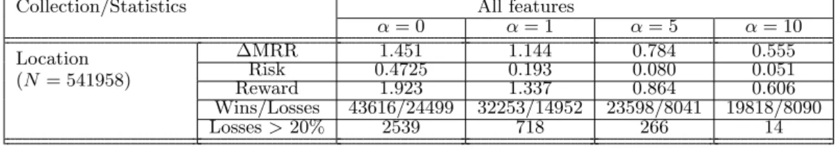
Tables 1 and 2 show summary retrieval quality and ro-bustness statistics for ranking on the MSLR and Location datasets. The gain over baseline effectiveness is broken down into its constituent Risk and Reward components. (Recall that Gain = Reward−Risk.) Unless otherwise noted, other summary stats are based on the top 10 results. The Wins/Losses row shows the counts of queries that contributed to the Reward vs Risk respectively.3 The ‘Loss > 20%’ statistic counts queries whose relative NDCG change over baseline NDCG was worse than -20%. Thus, smaller Loss numbers are better.

Risk, reward and wins/losses are relative to the baseline ranking. The NDCG@10 score for the BM25 baseline was 30.869. The ∆MRRscore for the Location minEntropy base-line is zero, since we report relative gains on that dataset for proprietary reasons.

As expected, there is a clear trade-off between overall re-trieval effectiveness and amount of risk reduction for both collections. As the risk-aversion parameter α is increased, the Wins/Losses row shows consistent reduction in losses, with a small decline in overall effectiveness (NDCG or ∆MRR). Note in particular that for the Location data, the chance of a query being hurt by more than 20% loss in ∆MRRcompared to the baseline vanishes almost to zero, while still retaining significant overall effectiveness gains.

5.6 Risk-reward tradeoff

Finding a re-ranking strategy that reduces variance com-pared to the baseline is easy - simply avoid re-ranking and always use the baseline ranking. In this case, the ∆MRR

will be zero, with zero risk. However, this obviously loses all the benefits of the re-ranking for queries that are actually helped by re-ranking. Our goal is to find optimal tradeoff strategies thatdominateother possible strategies for trading risk for reward.

Figure 2 shows our risk-sensitive objective in LambdaMart indeed dominates alternative effective strategies for selective re-ranking, as measured by the tradeoff curve for risk vs. gain for each collection. This tradeoff curve for the selec-tive re-ranking strategy is produced as a function of the fea-ture threshold (the minEntropy feafea-ture for Location queries, and maxBM25 feature for MSLR queries). As the feature threshold is lowered, more and more queries have the feature

3

We ignore queries with zero NDCG@10 difference from the baseline, with gains over baseline being a ‘Win’, and losses being a ‘Loss’.

(7)

Collection/Statistics All features α= 0 α= 1 α= 5 α= 10 MSLR (N = 10000) NDCG@1 46.166 45.835 44.615 43.658 NDCG@10 47.272 47.221 46.312 45.540 Risk 2.239 1.974 1.722 1.540 Reward 18.642 18.327 17.165 16.282 Wins/Losses 7512/1972 7630/1845 7613/1838 7645/1776 Loss>20% 740 684 630 573

Table 1: Summary of generalization performance over test folds for the MSLR dataset.

Collection/Statistics All features

α= 0 α= 1 α= 5 α= 10 Location (N= 541958) ∆MRR 1.451 1.144 0.784 0.555 Risk 0.4725 0.193 0.080 0.051 Reward 1.923 1.337 0.864 0.606 Wins/Losses 43616/24499 32253/14952 23598/8041 19818/8090 Losses>20% 2539 718 266 14

Table 2: Summary of generalization performance over test folds for the Location dataset.

value above the threshold and are re-ranked according to the baseline ranking. The tradeoff curve for the risk-sensitive re-ranking strategy is a function ofα. At α= 0, the risk-sensitive ranking coincides with the gain-only ranking. As

αis increased, the learned model exhibits a stronger pref-erence for the baseline, which acts like an increasing ‘soft’ query selection for the baseline ranking. The dotted Break Even line shows the break-even point where the tradeoff objective T= 0, and any result above the dashed Propor-tional Reduction line has the desirable property that it re-duces risk proportionally more than it rere-duces reward. The “near-optimal hull” curve represents an envelope of achiev-able tradeoffs that results from incorporating an automatic stopping strategy forα, details of which are given in Sec. 5.7. For both collections it is notable that the selective thresh-old re-ranking method performs significantly better than the break-even point. Additionally, since it lies above the Pro-portional Reduction line, it reduces risk proPro-portionally more than it reduces gain at almost all points of the curve. This is most evident at high values of the respective threshold features, when the ‘best’ queries amenable to that method are most likely to be selected. At much lower threshold values, it is clear that most queries do not benefit from re-ranking with the baseline feature, giving performance closer to break-even. Furthermore, while other selective personal-ization approaches could be taken, it is clear based on per-formance that the selective threshold method here provides an informative comparison point.

In turn, for the Location data, the risk-gain tradeoff achieved by risk-sensitive ranking completely dominates that of se-lective threshold re-ranking. For any given risk level, risk-sensitive ranking achieves significantly higher gain, and con-versely, for any given level of gain, it achieves that gain at much lower risk than the selective method. The results also show that the near-optimal hull dominates the selective method for both collections.

5.7 Guidance for setting the

α

parameter

A natural question is how to setα, or where one should stop trying new α’s. While α is a user-set parameter to

control risk, the question of where to stop can be approxi-mated. For any model, the risk can always be reduced by flipping a coin with probabilitypand applying the method given “heads” and the baseline given “tails”. Varyingp natu-rally both reduces the gain and the risk (e.g.,p= 0.20 yields 20% risk and 20% reward). Since we can apply the same logic to the gain only model, this leads to natural guidance in terms of the gain-to-risk ratio of the gain only model (GOM): when α = GainGOM/RiskGOM the original gain only model would yield a tradeoff objectiveT= 0. Further-more, randomly reducing the gain only model for greater values of α than this will continue to ensure the tradeoff objective remains non-negative. Thus, solutions withT >0 in the segmentα∈ [0,GainGOM/RiskGOM] are interesting non-trivial tradeoffs relative to the original gain-only model. To find the size of this segment of interest, we used per-formance over the training data. For MSLR, this yielded a value ofα= 27.9±1.3 and for Locationα= 4.0±0.04. Then starting from the maximal nearest computed αpoints (30 and 4 respectively) in the segment, we simulate the ran-dom reduction from there toward the origin and call this the “Near-Optimal Hull” line on the curves. This gives a more realistic picture of achievable tradeoffs.

5.8 Convergence rates

We discussed in Sec. 4.3.3 how adding our risk-sensitive objective to LambdaMart results in modifying the Lamb-daMart gradient in such a way that its magnitude is ampli-fied asαincreases, accelerating the learning rate for queries where baseline effectiveness is already high. Thus, we hy-pothesized that on average across all training queries, we would see faster convergence rates at high values ofα com-pared to low values ofα.

Figure 4 demonstrates that this phenomenon actually oc-curs on both collections, comparing the ranker convergence when α= 0 to setting α= 5. The x-axis indicates num-ber of iterations; the y-axis shows the overall NDCG@10 achieved at any given iteration (up to a maximum of 100 it-erations), averaged across all validation folds. Although the algorithm ultimately converged to very similar NDCG@10

(8)

1 1.5 2 2.5 3 3.5 Re war d (M RR ) Location

Risk-Sensitive with Near-Optimal Hull

0 0.2 0.4 0.6 0.8 1 1.2 1.4 0 0.2 0.4 0.6 0.8 1 Gain (MR R) Risk (MRR) Location Selective Risk-Sensitive Optimization Risk-Sensitive with Near-Optimal Hull Break-even Line Proportional Reduction Line

(a) Location: risk vs. gain

0 2 4 6 8 0 0.5 1 1.5 2 2.5 3 Re war d (N D CG @ 10 ) Risk (NDCG@10) 0 2 4 6 8 10 12 14 16 18 0 10 20 30 40 Ga in (R ewa rd -Ri sk)

Percentage Queries Measurably Different Gain vs Coverage 0 2 4 6 8 10 12 14 16 18 0 0.5 1 1.5 2 2.5 3 Gain ( NDC G@10) Risk (NDCG@10) MSLR Selective Risk-Sensitive Optimization Risk-Sensitive with Near-Optimal Hull Break-even Line Proportional Reduction Line

(b) MSLR: risk vs. gain

Figure 2: Risk/gain tradeoffs achieved by risk-sensitive LambdaMart learning vs. selective re-ranking for Location dataset (left), and MSLR dataset (right).

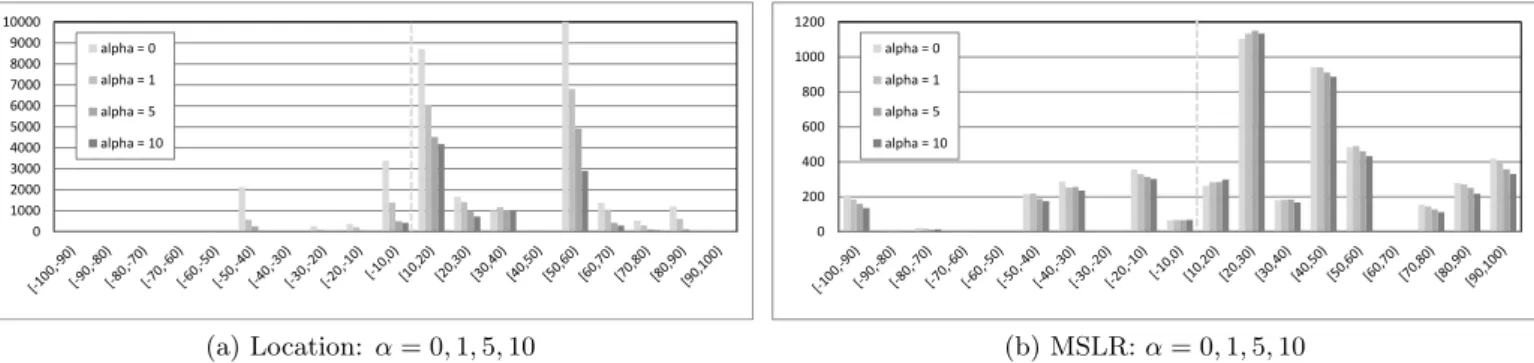
0 1000 2000 3000 4000 5000 6000 7000 8000 9000 10000 alpha = 0 alpha = 1 alpha = 5 alpha = 10 (a) Location: α= 0,1,5,10 0 200 400 600 800 1000 1200 alpha = 0 alpha = 1 alpha = 5 alpha = 10 (b) MSLR:α= 0,1,5,10

Figure 3: Helped-hurt histograms, showing how variance around baseline (dotted line) shrinks as the risk-aversion parameter

αis increased fromα= 0 (lightest bars) toα= 10 (darkest bars), for Location dataset (left), and MSLR dataset (right). Each histogram bucket corresponds to a different 10% range of loss/gain in effectiveness compared to that collection’s baseline, and contains four bars, corresponding to the number of queries helped or hurt for the four risk-reward tradeoff settings

α= 0,1,5,10. For clearer scaling the large spike of queries for the [0, 10) bucket has been omitted in both charts.

for both settings, the α= 5 runs converged faster for all folds on both collections. In the case of the Location data, the speed improvement was dramatic – learning withα= 5 took an average of 10.2 iterations to achieve 95% of the final convergence effectiveness, compared to 41.5 withα= 0. The improvement was smaller but still consistent across folds for the MSLR data: for example, learning withα= 5 reached NDCG@10 gain of 0.42 in an average of 25.4 iterations, com-pared with 33.4 iterations forα= 0.

5.9 Model consistency across risk levels

We now examine how rankings change with respect to the baseline results as the risk-aversion parameterαis increased. To measure change between rankings, we use Kendall’s tau distance, a standard distance between two ranked lists that corresponds to the (normalized) number of pairwise swaps required to move from one ranking to another. A large Kendall distance indicates low similarity to the baseline rank-ing, and conversely a small Kendall distance indicates a ranking that is very similar to the baseline ranking.

For illustration purposes, we binned Kendall distance val-ues into 10 bins from 0 to 9. Queries whose re-ranking is the same or very similar to the baseline ranking are put in Bin 0, while queries with re-rankings that are very different from the baseline are put into Bin 9, or an intermediate bin according to the Kendall distance.

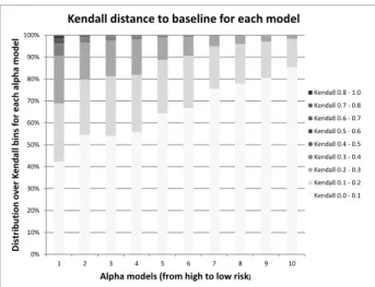
Figure 5 shows, for each value ofα, a distribution over Kendall bins using the location personalization dataset. It shows that as the permitted risk increases – alpha changes from high to low – more and more queries start to deviate significantly from the baseline. For example, the lower-risk model learned withα= 9 has 85% of the queries staying close to the baseline (bin 0), while the higher-risk model learned withα= 1 has only 42% of the queries close to the baseline ranking, with the remaining queries dispersed over much more diverse rankings with much larger Kendall distances from the baseline. This behavior can be explained in terms of risk/reward tradeoff. The higher-risk models have the in-centive to deviate significantly from the baseline in exchange for more drastic improvement in effectiveness (which is

(9)

val-1 0.34 0.36 0.38 0.4 0.42 0.44 0.46 1 11 21 31 41 51 61 71 81 91 ND CG Iterations alpha=10 alpha = 5 alpha = 0 (a) 2 0.65 0.67 0.69 0.71 0.73 0.75 0.77 0.79 0.81 0.83 1 5 9 ₁₃ ₁₇ ₂₁ ₂₅ ₂₉ ₃₃ ₃₇ ₄₁ ₄₅ ₄₉ ₅₃ ₅₇ ₆₁ ₆₅ ₆₉ ₇₃ ₇₇ ₈₁ ₈₅ ₈₉ ₉₃ ₉₇ NDCG Iterations Reward only Risk aware (alpha=8) (b)

Figure 4: Risk-sensitive model (high α) consistently con-verges faster than reward-only objective (α= 0), for both the MSLR dataset (top) and Location dataset (bottom). Each iteration point is averaged over all validation folds.

ued more by the tradeoff metric under a lowαvalue); while low-risk models (highαvalue) tend to stay close to baseline, since risk is aggressively penalized by the tradeoff metric un-der largeαand there is no incentive to significantly deviate from baseline (even if that means a higher gain) due to the potentially large penalty incurred from it. This fact is also confirmed by results shown in Table 2, where the higher-risk model trades off more robustness for effectiveness.

Moreover, in models that heavily penalize risk, the re-ranked results for a particular query may deviate signifi-cantly from baseline, but only under the condition that the reward (NDCG gain) acquired as a result of the deviation must be high enough to outweigh the increased risk. We can see this behavior in the risk-sensitive modelα= 9. Al-though a majority of the queries are in Bin 0 (near base-line), the overall NDCG gain is moderate and the overall risk is the lowest among all models. Also interesting is that as Kendall distance increases, the safe model tends to have the largest reward among other models under same kendall distance. For safe model (α= 9), reward is 0.00371 under kendall bin 2, which is the highest among other models in the same Kendall bin 2. Thus, one potential application of this type of cross-model analysis might be to use the consis-tency across different models to produce the best reranking model for each query.

0% 10% 20% 30% 40% 50% 60% 70% 80% 90% 100% 1 2 3 4 5 6 7 8 9 10 Di str ibu ti on ov er K enda ll bin s for ea ch al pha model

Alpha models (from high to low risk)

Kendall distance to baseline for each model

Kendall 0.8 - 1.0 Kendall 0.7 - 0.8 Kendall 0.6 - 0.7 Kendall 0.5 - 0.6 Kendall 0.4 - 0.5 Kendall 0.3 - 0.4 Kendall 0.2 - 0.3 Kendall 0.1 - 0.2 Kendall 0.0 - 0.1

Figure 5: Distributions of Kendall distances to baseline ranking, for increasing values of the risk parameter α (lo-cation dataset). For high-risk models (α = 1), only 42% of queries have re-ranked results that remain very close to the baseline ranking (Bin 0), compared to low-risk (α= 10) models having 90% of queries with results very close to the baseline.

6. DISCUSSION AND FUTURE WORK

In this study we gave a definition of ‘risk’ in terms of the size of the downside tail of a distribution over a specific performance measure: NDCG. However, our framework is not limited to that choice and can address a much broader family of scenarios.

First, the risk and reward parts of the ranking objective may address other performance aspects of the results rank-ing, as long as the combined measure is consistent.

Second, we can look beyond strictly performance-related definitions of risk to include other properties of result sets. For example, thechurn of a set of results for a given query refers to undesirable and unexpected volatility in a given query’s results after re-ranking, even (or especially) when the rankings of the best relevant documents - and thus over-all performance - might be unchanged or only minimover-ally re-duced. All things being equal, given two rankings with the same retrieval performance, we may prefer the one that gives less churn compared to a baseline ranking. Thus, the ‘risk’ of ranking might be defined using a ranking dissimilarity measure such as Kendall’s tau compared to the baseline, in-stead of the strictly performance-based difference in NDCG we used here.

Third, another assumption we made was that reducing downside variance was a desirable goal. In general, this is true. However, there may be some retrieval tasks where it is beneficial to have an objective that tries to increase

up-side variance, even if this leads to an increased chance of

large errors. Typically this will be in cases where a greater diversity of retrieval hypotheses is desirable as part of a larger precision-oriented system. For example, a search en-gine, acting as one source among several that provides can-didate documents to a question-answering application, may be more likely to find high-reward documents if it does more aggressive promotion from deep in the original ranking.

(10)

Finally, we note that our use of an objective that mini-mizes negative outcomes with respect to a baseline is a spe-cial case of regret-based learning. In particular, we could generalize our risk-reward objective to minimize the average loss over the worstX% tail of negative outcomes, instead of all negative outcomes, and this could be viewed as a mini-max regret objective - with connections to the widely-used Conditional Value-at-Risk objective from financial optimiza-tion. Beyond ranking, we believe this family of robust ob-jectives deserves wider consideration in IR, with potential applicability to tasks such as query rewriting, federated re-source selection, meta-search and others, where risk-reward scenarios exist and finding the highest-quality operational tradeoffs is critical.

7. CONCLUSIONS

We presented a general approach for improving the ro-bustness of learned rankers by performing risk-sensitive op-timization of ranking models. Our opop-timization adds a novel additional ranking objective that minimizes downside risk relative to a given baseline, in addition to the standard ob-jective factor that maximizes average effectiveness across queries. Our approach can be viewed as a way to con-trol the robustness/effectiveness tradeoff in learning-to-rank approaches. Thus, it generalizes the standard learning to rank approaches as special cases that do not consider ro-bustness. Our robustness metric is orthogonal to previous multi-objective learning to rank metrics for capturing differ-ent facets for search, since robustness is definedusing stan-dard facet-based and IR performance measureswith respect toa baseline model. We proved the theoretical consistency of the proposed tradeoff measure and designed a principled learning to rank approach, using boosted regression trees, to optimize it. Our approach can be potentially applied to a wide range of applications in learning-to-rank by plugging in different baseline models. Furthermore, by performing an extensive empirical evaluation using both public and pro-prietary datasets we demonstrated that our robust models achieve significant benefits in learning rate, robustness, and reliability over existing methods.

8. REFERENCES

[1] P. N. Bennett, F. Radlinski, R. W. White, and E. Yilmaz. Inferring and using location metadata to personalize web

search. InSIGIR, pages 135–144, 2011.

[2] R. Bhattacharjee and A. Goel. Algorithms and incentives for

robust ranking. InSODA 2007.

[3] J. Bian, X. Li, F. Li, Z. Zheng, and H. Zha. Ranking specialization for web search: a divide-and-conquer approach

by using topical ranksvm. InWWW, pages 131–140, 2010.

[4] J. Bian, T.-Y. Liu, T. Qin, and H. Zha. Ranking with

query-dependent loss for web search. InWSDM, pages 141–150,

2010.

[5] C. Burges, T. Shaked, E. Renshaw, A. Lazier, M. Deeds, N. Hamilton, and G. Hullender. Learning to rank using

gradient descent. InICML, pages 89–96, 2005.

[6] C. J. C. Burges. From RankNet to LambdaRank to LambdaMART: An Overview. Technical report, Microsoft Research, 2010.

[7] C. J. C. Burges, R. Ragno, and Q. V. Le. Learning to Rank

with Nonsmooth Cost Functions. InNIPS, pages 193–200. MIT

Press, 2006.

[8] S. B¨uttcher, C. L. A. Clarke, and B. Lushman. Term proximity

scoring for ad-hoc retrieval on very large text collections. In SIGIR, pages 621–622, 2006.

[9] O. Chapelle and Y. Chang. Yahoo! learning to rank challenge

overview.Journal of Machine Learning Research

-Proceedings Track, 14:1–24, 2011.

[10] K. Collins-Thompson. Reducing the risk of query expansion via

robust constrained optimization. InCIKM 2009, pages

837–846.

[11] K. Collins-Thompson, P. N. Bennett, R. W. White, S. de la Chica, and D. Sontag. Personalizing web search results by

reading level. InCIKM, pages 403–412, 2011.

[12] S. Cronen-Townsend, Y. Zhou, and W. B. Croft. Predicting

query performance. InSIGIR, pages 299–306.

[13] N. Dai, M. Shokouhi, and B. D. Davison. Learning to rank for

freshness and relevance. InSIGIR, pages 95–104, 2011.

[14] P. Donmez, K. M. Svore, and C. J. C. Burges. On the local

optimality of lambdarank. InSIGIR, pages 460–467, 2009.

[15] Z. Dou, R. Song, and J.-R. Wen. A large-scale evaluation and

analysis of personalized search strategies. InWWW, pages

581–590, 2007.

[16] E. N. Efthimiadis. Chapter: Query expansion.Annual Review

of Information Science and Technology, 31:121–187, 1996. [17] J. H. Friedman. Greedy function approximation: A gradient

boosting machine.Annals of Statistics, 29:1189–1232, 2000.

[18] X. Geng, T.-Y. Liu, T. Qin, A. Arnold, H. Li, and H.-Y. Shum.

Query dependent ranking using k-nearest neighbor. InSIGIR,

pages 115–122, 2008.

[19] F. Gey. Inferring probability of relevance using the method of

logistic regression. InProc. 17th SIGIR Conference, 1994.

[20] Q. Guo, R. W. White, S. Dumais, J. Wang, and B. Anderson. Predicting query performance using query, result, and user

interaction features. InRIAO, 2010.

[21] C. Hauff, D. Hiemstra, and F. de Jong. A survey of

pre-retrieval query performance predictors. InCIKM, pages

1419–1420, 2008.

[22] C. Kang, X. Wang, J. Chen, C. Liao, Y. Chang, B. L. Tseng, and Z. Zheng. Learning to re-rank web search results with

multiple pairwise features. InWSDM’11, pages 735–744, 2011.

[23] B. Knijnenburg, M. C. Willemsen, Z. Gantner, H. Soncu, and C. Newell. Explaining the user experience of recommender

systems.J. of User Modeling and User-Adapted Interaction

(UMUAI), 22, 2011.

[24] F. Li, X. Li, S. Ji, and Z. Zheng. Comparing both relevance and

robustness in selection of web ranking functions. InSIGIR ‘09,

pages 648–649, 2009.

[25] T.-Y. Liu. Learning to rank for information retrieval.

Foundations and Trends in Information Retrieval, 3(3), 2009. [26] Y. Lv, C. Zhai, and W. Chen. A boosting approach to

improving pseudo-relevance feedback. InSIGIR, pages 165–174,

2011.

[27] D. Metzler and W. B. Croft. A Markov Random Field model

for term dependencies. InProc. 28th SIGIR Conference, pages

472–479, 2005.

[28] J. Ponte and W. B. Croft. A language modeling approach to

information retrieval. InProc. 21st SIGIR Conference, pages

275–281, 1998.

[29] S. Robertson, S. Walker, S. Jones, M. M. Hancock-Beaulieu,

and M. Gatford. Okapi at TREC-3. InProc. 3rd TREC

Conference, pages 109–126, 1994.

[30] R. Steuer.Multiple Criteria Optimization: Theory,

Computation and Application. John Wiley, 1986.

[31] K. M. Svore, M. N. Volkovs, and C. J. Burges. Learning to rank

with multiple objective functions. InWWW, pages 367–376,

2011.

[32] T. Tao and C. Zhai. An exploration of proximity measures in

information retrieval. InProc. 30th SIGIR Conference, 2007.

[33] J. Teevan, S. T. Dumais, and E. Horvitz. Potential for

personalization.ACM TOCHI, 17(1), 2010.

[34] E. M. Voorhees. The trec robust retrieval track.SIGIR Forum,

39(1):11–20, June 2005.

[35] J. Wang and J. Zhu. Portfolio theory of information retrieval.

InSIGIR. ACM, 2009.

[36] R. W. White, P. N. Bennett, and S. T. Dumais. Predicting short-term interests using activity-based search context. In CIKM, pages 1009–1018, 2010.

[37] Q. Wu, C. J. Burges, K. M. Svore, and J. Gao. Adapting

boosting for information retrieval measures.Information

Retrieval, 13:254–270, June 2010.

[38] Y. Zhou and W. B. Croft. Query performance prediction in web

search environments. InResearch and Development in

Information Retrieval, pages 543–550, 2007.

[39] J. Zhu, J. Wang, I. J. Cox, and M. J. Taylor. Risky business: modeling and exploiting uncertainty in information retrieval. In SIGIR. ACM, 2009.

Robust Ranking Models via Risk-Sensitive Optimization