Real parameter optimization by an effective differential evolution algorithm

ORIGINAL ARTICLE

Real parameter optimization by an effective

differential evolution algorithm

Ali Wagdy Mohamed

*

_{, Hegazy Zaher Sabry}

_{, Tareq Abd-Elaziz}

a

Statistics Department, Faculty of Science, King Abdulaziz University, P.O. Box 80203, Jeddah 21589, Saudi Arabia b

Operations Research Department, Institute of Statistical Studies and Research, Cairo University, Giza, Egypt c

Mathematical Statistics Department, Institute of Statistical Studies and Research, Cairo University, Giza, Egypt Received 23 June 2012; revised 12 December 2012; accepted 1 January 2013

Available online 1 February 2013

KEYWORDS Differential evolution; Best–worst mutation; Global optimization; Modified BGA mutation

Abstract This paper introduces an Effective Differential Evolution (EDE) algorithm for solving real parameter optimization problems over continuous domain. The proposed algorithm proposes a new mutation rule based on the best and the worst individuals among the entire population of a particular generation. The mutation rule is combined with the basic mutation strategy through a linear decreasing probability rule. The proposed mutation rule is shown to promote local search capability of the basic DE and to make it faster. Furthermore, a random mutation scheme and a modified Breeder Genetic Algorithm (BGA) mutation scheme are merged to avoid stagnation and/or premature convergence. Additionally, the scaling factor and crossover of DE are introduced as uniform random numbers to enrich the search behavior and to enhance the diversity of the pop-ulation. The effectiveness and benefits of the proposed modifications used in EDE has been exper-imentally investigated. Numerical experiments on a set of bound-constrained problems have shown that the new approach is efficient, effective and robust. The comparison results between the EDE and several classical differential evolution methods and state-of-the-art parameter adaptive differ-ential evolution variants indicate that the proposed EDE algorithm is competitive with , and in some cases superior to, other algorithms in terms of final solution quality, efficiency, convergence rate, and robustness.

Ó2013 Faculty of Computers and Information, Cairo University. Production and hosting by Elsevier B.V. All rights reserved.

1. Introduction

Differential Evolution (DE) is a stochastic population-based search method, proposed by Storn and Price [1]for solving non-linear, high-dimensional and complex computational opti-mization problems. DE is considered the most recent EAs for solving real-parameter optimization problems [2]. DE has many advantages including simplicity of implementation, reli-able, robust, and in general is considered as an effective global * Corresponding author at: Statistics Department, Faculty of

Sciences, King Abdulaziz University, P.O. Box 80203, Jeddah 21589, Saudi Arabia. Tel.: +966 556269723, +20 1005157657.

E-mail address:[email protected](A.W. Mohamed).

Peer review under responsibility of Faculty of Computers and Information, Cairo University.

Production and hosting by Elsevier

Cairo University

Egyptian Informatics Journal

www.sciencedirect.com

1110-8665Ó2013 Faculty of Computers and Information, Cairo University. Production and hosting by Elsevier B.V. All rights reserved.

optimization algorithm[3]. Therefore, it has been used in many real-world applications, such as flow shop scheduling[4], ma-chine intelligence applications[5], financial markets dynamic modeling[6], pattern recognition studies[7], signal processing implementations[8], data mining[9], power systems[10], fuzzy logic systems[11], and many others. DE, nevertheless, also has shortcomings as all other intelligent techniques. Firstly, while the global exploration ability of DE is considered adequate, its local exploitation ability is regarded weak and its conver-gence velocity is too low[12]. Secondly, DE suffers from the problems of premature convergence and stagnation[13,14]. Fi-nally, DE is sensitive to the choice of the control parameters and it is difficult to adjust them for different problems. More-over, like other evolutionary algorithms, DE performance de-creases as search space dimensionality inde-creases[13]. Indeed, due to the above drawbacks, a lot of researchers have pro-posed to overcome these problems and to improve the overall performance of the DE algorithm. The choice of DE’s control variables has been discussed by Storn and Price[1]who sug-gested a reasonable choice for NP(population size) between 5D and 10D (D being the dimensionality of the problem), and 0.5 as a good initial value ofF(mutation scaling factor). The effective value ofFusually lies in the range between 0.4 and 1. As for the CR (crossover rate), an initial good choice of CR = 0.1; however, since a large CR often speeds conver-gence, it is appropriate to first try CR as 0.9 or 1 in order to check if a quick solution is possible. After many experimental analysis, Ga¨mperle et al.[15]recommended that a good choice forNP is between 3D and 8D, withF= 0.6 and CR lies in [0.3, 0.9]. Contrarily, Ro¨nkko¨nen et al. [16] concluded that F= 0.9 is a good compromise between convergence speed and convergence probability. Additionally, CR depends on the nature of the problem, so CR with a value between 0.9 and 1 is suitable for non-separable and multimodal objective functions, while a value of CR between 0 and 0.2 when the objective function is separable. Due to the contradiction claims that can be seen from the literature, some techniques have been designed to adjust control parameters in adaptive or self-adap-tive manner instead of trial-and-error procedure. A Fuzzy Adaptive Differential Evolution (FADE) algorithm was pro-posed by Liu and Lampinen[17]. They introduced fuzzy logic controllers to adjust crossover and mutation rates. Numerical experiments and comparisons on a set of well known bench-mark functions showed that the FADE Algorithm outper-formed basic DE algorithm. Likewise, Brest et al. [18] proposed an efficient technique, called jDE, for self-adapting control parameter settings by encoding the parameters into each individual and adapting them by means of evolution. The results showed that jDE is better than, or at least compa-rable to, the standard DE algorithm (FADE) algorithm and other evolutionary algorithms from the literature when consid-ering the quality of the solutions obtained. In the same con-text, Omran et al [19] proposed a Self-adaptive Differential Evolution (SDE) algorithm. The scaling factor F is self-adapted using a mutation rule similar to the mutation operator in the basic DE. The experiments conducted showed that SDE generally outperformed DE algorithms and other evolutionary algorithms. Zaharie [20] introduced an adaptive DE (ADE) algorithm based on the idea of controlling the population diversity and implemented a multi-population approach Ali and To¨rn[21]proposed a new DE algorithm with two evolving

populations. The crossover rate CR has been empirically stud-ied and set equal to 0.5. Unlike CR, the value of the scaling factorFis adaptively calculated at each generation by using fit-ness-based adaptation scheme based on the maximum and minimum objective function values over the individuals of populations. In a similar way, the scale factor local search dif-ferential evolution (SFLSDE) is presented by Neri and Tirro-nen [22]. It is a DE-based memetic algorithm (MA) which employs within a self-adaptive scheme, two local search algo-rithms which are golden section search and hill climbing search. These local search algorithms aim at detecting a value of the scale factor corresponding to an offspring with a high performance, while the generation is executed. The local search algorithms thus assist in the global search and generate off-spring with high performance which are subsequently sup-posed to promote the generation of enhanced solutions within the evolutionary framework. The efficiency of the pro-posed algorithm seems to be very high especially for large scale problems and complex fitness landscapes. SaDE (self-adaptive differential evolution) is proposed by Qin et al.[23]. The main idea of SaDE is to simultaneously implement two mutation schemes: ‘‘DE/rand/1/bin’’ and ‘‘DE/best/2/bin’’ and also to adapt mutation and crossover parameters. The Performance of SaDE evaluated over a suite of 26 several benchmark prob-lems and it was compared with the conventional DE and three adaptive DE variants. The presented experimental results dem-onstrated that SaDE was more effective in obtaining better quality solutions and had higher success rate. Similarly, Zhang and Sanderson [24]introduced a new Differential Evolution (DE) algorithm, named JADE, to improve optimization per-formance by implementing a new mutation strategy ‘‘DE/cur-rent-to-pbest’’ with optional external archive and updating control parameters in an adaptive manner. Simulation results show that JADE is better than, or at least comparable to, other classic or adaptive DE algorithms, Particle swarm and other evolutionary algorithms from the literature in terms of convergence performance for a set of 20 benchmark problems. Recently, motivated by the recent success of diverse self-adaptive DE approaches, Das et al. [25] developed a self-adaptive DE, called FiADE. In FiADE, an effective adaptation technique for tuning both Fand Cr is proposed, on the run, without any user intervention. The adaptation strategy is based on the objective function value of individuals in the DE population. Comparison with the best-known and expensive variants of DE over fourteen well-known numerical benchmarks and one real-life engineering problem reflects the superiority of proposed parameter tuning scheme in terms of accuracy, convergence speed, and robustness. Practically, from the literature, it can be observed that the main modifications, improvements and developments on DE focus on adjusting control parameters in adaptive or self-adaptive manner. How-ever, a few enhancements have been implemented to modify the standard mutation strategies or to propose new mutation rules so as to enhance the local search ability of DE or to over-come the problems of stagnation or premature convergence

[13,26–29]. Consequently, proposing new mutations and

adjusting control parameters are still an open challenge direc-tion of research [30–36]. Therefore, in order to improve the global performance of basic DE, this research uses a new mutation rule to enhance the local exploitation tendency and to improve the convergence rate of the algorithm. The scaling

factor and the crossover of DE are also introduced as uniform random number to enrich the whole search space and to enhance the diversity of the population. In order to avoid the stagnation and the premature convergence issues through generations, modified BGA mutation and a random mutation are embedded into the proposed EDE algorithm. Numerical experiments and comparisons conducted in this research effort on a set of well-known high dimensional benchmark functions indicate that the proposed Improved Differential Evolution (EDE) algorithm is superior and competitive with conven-tional DE and several state-of-the-art parameter adaptive DE variants particularly in the case of high dimensional com-plex optimization problems. The rest of the paper is organized as follows. In Section 2, the standard DE algorithm is intro-duced. Next, in Section 3, the new EDE algorithm is described in detail. Section 4 reports on the computational results of test-ing benchmark functions and on the comparison with other techniques is discussed. Section 5 discusses the effectiveness of the proposed modifications. Finally, conclusions and future works are drawn in Section 6.

2. The differential evolution algorithm

A bound constrained global optimization problem can be de-fined as follows[37]:

minfðXÞ; X¼ ½x1;. . .;xn; S:t:xj2 ½aj;bj; j¼1;2;. . .n; ð1Þ wherefis the objective function,Xis the decision vector con-sisting ofnvariables, andajandbjare the lower and upper bounds for each decision variable, respectively. Virtually, there are several variants of DE[1]. In this paper, we use the scheme which can be classified using the notation as DE/rand/1/bin strategy[1,18]. This strategy is the most often used in practice. A set of D optimization parameters is called an individual, which is represented by a D-dimensional parameter vector. A population consists of NP parameter vectors xG

i, i= 1, 2, ... ,NP. Gdenotes one generation. NP is the number of members in a population. It is not changed during the evolu-tion process. The initial populaevolu-tion is chosen randomly with uniform distribution in the search space. DE has three opera-tors: mutation, crossover and selection. The crucial idea be-hind DE is a scheme for generating trial vectors. Mutation and crossover operators are used to generate trial vectors, and the selection operator then determines which of the vectors will survive into the next generation[18].

2.1. Initialization

In order to establish a starting point for the optimization pro-cess, an initial population must be created. Typically, each decision parameter in every vector of the initial population is assigned a randomly chosen value from the boundary constraints:

x0

ij¼ajþrandj ðbjajÞ ð2Þ whererandjdenotes a uniformly distributed number between [0, 1], generating a new value for each decision parameter.aj and bj are the lower and upper bounds for the jth decision parameter, respectively.

2.2. Mutation

For each target vectorxG

i, a mutant vectorv Gþ1

i is generated according to the following:

vGþ1 i ¼x G r1þF ðx G r2x G r3Þ; r1–r2–r3–i ð3Þ

with randomly chosen indices andr1,r2,r3e{1, 2, ... ,NP}. Note that these indices must be different from each other and from the running indexiso thatNPmust be at least four. Fis a real number to control the amplification of the difference vectorðxG

r2x

G

r3Þ. According to[30], the range ofFis in [0, 2].

If a component of a mutant vector goes off the search space, then the value of this component is generated a new using(2). 2.3. Crossover

The target vector is mixed with the mutated vector, using the following scheme, to yield the trial vectoruGþ1

i . uG_ijþ1¼ v

G

ij;randðjÞ CR or j¼randnðiÞ; xG

ij;randðjÞ>CR and j–randnðiÞ; (

ð4Þ where j= 1, 2, ... ,D,rand(j)e[0, 1] is the jth evaluation of a uniform random generator number.CRe[0, 1] is the crossover probability constant, which has to be determined by the user. randn(i)e{1, 2, ... ,D} is a randomly chosen index which en-sures thatuGþ1

i gets at least one element fromvGþ

1

i ; otherwise no new parent vector would be produced and the population would not alter.

2.4. Selection

DE adapts a greedy selection strategy. If and only if the trial vectoruGþ1

i yields a better fitness function value thanx G i, then uGþ1

i is set toxGþ

1

i . Otherwise, the old vectorxGi is retained. The selection scheme is as follows (for a minimization problem):

xGþ1 i ¼ uGþ1 i ;fðuGiþ1Þ<fðxGiÞ; xG i;fðuGiþ1ÞPfðxGiÞ: ð5Þ

3. Effective differential evolution algorithm

All evolutionary algorithms, including DE, are stochastic popu-lation-based search methods. Accordingly, there is no guarantee to reach the global optimal solution all the times. Nonetheless, adjusting control parameters such as the scaling factor, the crossover rate and the population size, alongside developing an appropriate mutation scheme, can considerably improve the search capability of DE algorithms and increase the possibil-ity of achieving promising and successful results in complex and large scale optimization problems. Therefore, in this paper, four modifications are introduced in order to significantly enhance the overall performance of the standard DE algorithm. 3.1. Modification of mutations

Practical experience through many developed evolutionary algorithms and experimental investigation prove that a success of the population-based search algorithms is based on balanc-ing two contradictory aspects: global exploration and local exploitation[13]. Moreover, the mutation scheme plays a vital

role in the DE search capability and the convergence rate. However, even though the DE algorithm has good global exploration ability, it suffers from weak local exploitation abil-ity as well as its convergence velocabil-ity is still too low as the re-gion of the optimal solution is reached[26]. Obviously, from the mutation Eq. (3), it can be observed that three vectors are chosen at random for mutation and the base vector is then selected at random among the three. Consequently, the basic mutation strategy DE/rand/1/bin is able to maintain popula-tion diversity and global search capability, but it slows down the convergence of DE algorithms. Hence, in order to enhance the local search tendency and to accelerate the convergence of DE technique, a new mutation rule is proposed based on the best and the worst individuals among the entire population of a particular generation. The modified mutation scheme is as follows: vGþ1 i ¼x G b þF x G r x G w ð6Þ wherexG

r is a random chosen vector andxGb andxGware the best and worst vectors in the entire population, respectively. This modification is intended to replace the random base vector xG

r1andx

G

r3 in the mutation Eq.(3)by the best and worst

indi-vidual vectors with the best and worst fitness, respectively (i.e. lowest and highest objective function value for minimization problem) in the population at generationG. This process ex-plores the region around the best vector. Besides, it also favors exploitation ability since the mutant individuals are strongly attracted around the current best vector and at same time en-hances the convergence speed. Obviously, from mutation Eq. (6), it can be observed that the new mutation scheme has two benefits. Firstly, for the difference vector, the perturbation part of the mutation, the global solution can be easily reached if all vectors follow the direction of the better individual vector besides they also follow the opposite direction of the worst individual vector. Therefore, the directed perturbation in the proposed mutation resembles the concept of gradient as the difference vector is oriented from the worst vector to the better vectors[38]. Secondly, indeed, the new mutation process ex-ploits the nearby region around xG

b in the direction of ðxG

r xGwÞby different weights as will be discussed in the next subsection. As a result, the new mutation rule has better local search ability and faster convergence rate. The new mutation strategy is embedded into the DE algorithm and it is combined with the basic mutation strategy DE/rand/1/bin through a non-linear decreasing probability rule as follows:

If uð0;1Þ 1 G GEN Then ð7Þ vGþ1 i ¼x G b þF x G r x G w ð8Þ Else v_iGþ1¼xG_r1þFx_rG₂xG_r3 ð9Þ whereFis a uniform random variables,u(0, 1) returns a real number between 0 and 1 with uniform random probability dis-tribution andGis the current generation number, andGENis the maximum number of generations. From the above scheme, it can be realized that for each vector, only one of the two strategies is used for generating the current trial vector, depending on a uniformly distributed random value within the range (0, 1). For each vector, if the random value is smaller

than 1 G GEN

, then the basic mutation is applied. Otherwise, the proposed one is performed. Of course, it can be seen that, from Eq.(7), the probability of using one of the two mutations is a function of the generation number, so 1 G

GEN

can be gradually changed from 1 to 0 in order to favor, balance, and combine the global search capability with local search ten-dency. The strength and efficiency of the above scheme is based on the fact that, at the beginning of the search, two mutation rules are applied but the probability of the basic mutation rule to be used is greater than the probability of the new strategy. So, it favors exploration. Then, in the middle of the search, through generations, the two rules are approxi-mately used with the same probability. Accordingly, it bal-ances the search direction. Later, two mutation rules are still applied but the probability of the proposed mutation to be per-formed is greater than the probability of using the basic one. Finally, it enhances exploitation. Therefore, at any particular generation, both exploration and exploitation aspects are done in parallel. On the other hand, although merging a local muta-tion scheme into a DE algorithm can enhance the local search ability and speed up the convergence velocity of the algorithm, it may lead to a premature convergence and/or to get stagnant at any point of the search space especially with high dimen-sional problems [13,27]. For this reason, random mutation and a modified BGA mutation are merged and incorporated into the DE algorithm to avoid both cases at early or late stages of the search process. Generally, in order to perform random mutation on a chosen vectorxiat a particular gener-ation, a uniform random integer numberjrandbetween [1,D] is first generated and than a real number between (bj–aj) is calcu-lated. Then, thejrandvalue from the chosen vector is replaced by the new real number to form a new vectorx0_{. The random}

mutation can be described as follows. x0 j¼ ajþrandj ðbjajÞ j¼jrand xj otherwise ; j¼1;. . .;D ð10Þ

Therefore, it can be deduced from the above equation that random mutation increases the diversity of the DE algorithm as well decreases the risk of plunging into local point or any other point in the search space. In order to perform BGA mutation, as discussed in[39], on a chosen vectorxiat a par-ticular generation, a uniform random integer numberjrand be-tween [1,D] is first generated and then a real number between 0.1Æ(bj–aj)Æais calculated. Then, thejrandvalue from the chosen vector is replaced by the new real number to form a new vector x0

i. The BGA mutation can be described as follows. x0_j¼ xjþ0:1 ðbjajÞ a j¼jrand

xj otherwise

; j¼1;. . .;D ð11Þ

The + orsign is chosen with probability 0.5.ais com-puted from a distribution which prefers small values. This is realized as follows.

a¼X

15

k¼0

ak2k; ak2 f0;1g ð12Þ

Before mutation, we setai= 0. Afterwards, eachaiis mu-tated to 1 with probabilitypa= 1/16. Onlyakcontributes to the sum as in Eq.(12). On average, there will be just oneak with value 1, sayam, thenais given bya= 2m. In this paper, the modified BGA mutation is given as follows:

x0 j¼ xjrandj ðbjajÞ a j¼jrand xj otherwise ; j¼1;. . .;D ð13Þ where the factor of 0.1 in Eq.(11)is replaced by a uniform ran-dom number generator in the range [0, 1], because the constant setting of 0.1 (bj–aj) is not suitable. However, the probabilistic setting ofrandj ðbjajÞenhances the local search capability with small random numbers besides it still has an ability to jump to another point in the search space with large random numbers so as to increase the diversity of the population. Prac-tically, no vector is subject to both mutations in the same gen-eration, and only one of the above two mutations can be applied with the probability of 0.5. However, both mutations can be performed in the same generation with two different vectors. Therefore, at any particular generation, the proposed algorithm has the chance to improve the exploration and exploitation abilities. Furthermore, in order to avoid stagna-tion as well as premature convergence and to maintain the con-vergence rate, a new mechanism for each solution vector is proposed that satisfies the following condition: if the difference between two successive objective function values for any vector except the best one at any generation is less than or equal a predetermined leveldfor predetermined allowable number of generationsK, then one of the two mutations is applied with equal probability of (0.5). This procedure can be expressed as follows:

If jfcfpj dforKgenerations;then

Ifðuð0;1Þ 0:5Þ;then ð14Þ x0 j¼ ajþrandjðbjajÞj¼jrand xj otherwise ; j¼1;...;D; ðRandom MutationÞ ð15Þ Else x0 j¼ xjrandj ðbjajÞaj¼jrand xj otherwise

;j¼1;...;D;ðModified BGA mutationÞ ð16Þ wherefcandfpindicate current and previous objective function values, respectively.

After many experiments, in order to make a comparison with other algorithms with all dimensions, we observed that d= E06 and K= 25 generations are the best settings for these two parameters over all benchmark problems and these values seem to maintain the convergence rate as well as avoid stagnation and/or premature convergence in case they occur. Indeed, these parameters were set to their mean values. In this paper, these settings were fixed for all dimensions without tun-ing them to their optimal values that may attain good solutions better than the current results and improve the performance of the algorithm over all the benchmark problems.

3.2. Modification of scaling factor

In the mutation Eq.(3), the constant of differentiationFis a scaling factor of the difference vector. It is an important param-eter that controls the evolving rate of the population. In the ori-ginal DE algorithm in[2], the constant of differentiationFwas chosen to be a value in [0, 2]. The value ofFhas a considerable influence on exploration: small values ofFlead to premature convergence, and high values slow down the search[38]. How-ever, to the best of our knowledge, there is no optimal value of

Fthat has been derived based on theoretical and/or systematic study using all complex benchmark problems. It can be clearly observed from mutation Eq.(6)that the difference vector is a di-rected difference vector from the worst to the better vectors. Hence,Fmust be a positive value in order to bias the search direction for the trial vectors in the same direction. In fact, if the value ofFis kept constant value the diversity of the popula-tion is extremely decreased during the search process as the all the vectors are perturbed by the same difference vector compo-nent. Therefore, Instead of keepingFconstant during the search processFis set as a random variable for each trial vector so as to perturb the best vectorxG

b by different directed weights. There-fore,Fis introduced as a uniform random variable in [0.2, 0.8], where the range is determined empirically. Accordingly, this range ensures both exploitation tendency (with smallFvalues) and exploration ability (with largeFvalues). In order to reduce the number of parameters of the proposed algorithmFis also used with basic mutation.

3.3. Modification of the crossover rate

The crossover operator, as in Eq.(4), shows that the constant crossover (CR) reflects the probability with which the trial indi-vidual inherits the actual indiindi-vidual’s genes[38]. The constant crossover (CR) practically controls the diversity of the popula-tion. If the CR value is relatively high, this will increase the pop-ulation diversity and improve the convergence speed. Nevertheless, the convergence rate may decrease and/or the population may prematurely converge. On the other hand, small values of CR increase the possibility of stagnation and slow down the search process. Additionally, at the early stage of the search, the diversity of the population is large because the vectors in the population are completely different from each other and the variance of the whole population is large. There-fore, the CR must take a small value in order to avoid the exceed-ing level of diversity that may result in premature convergence and slow convergence rate. Then, through generations, the var-iance of the population will decrease as the vectors in the popu-lation become similar. Thus, in order to advance diversity and increase the convergence speed, the CR must be a large value. Based on the above analysis and discussion, and in order to bal-ance between the diversity and the convergence rate, CR is intro-duced as a uniform random variable in [0.5, 0.9], where the range is determined empirically and as extensively used in the

litera-ture[2,17,15,18]. In order to reduce the number of parameters

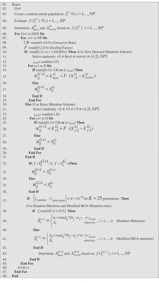
of the proposed algorithm CR is also used with basic mutation. The description of EDE is presented inFig. 1.

4. Numerical experiments and comparisons 4.1. Benchmark functions

In order to evaluate the performance and show the efficiency and superiority of the proposed algorithm (EDE), 14 well-known benchmark test functions mentioned in[40,23]are used. All these functions are minimization problems. Among the func-tions,f1–f4are unimodal and functionsf5–f14are multimodal. However, the generalized Rosenbrock’s functionf3is a multi-modal function when D > 3[41]. These 14 test functions are dimension wise scalable. Definitions of the Benchmark Prob-lems are as follows:

(1) Shifted sphere function f1ðxÞ ¼ XD i¼1 z2 i; z¼xo;o¼ ½o1;o2;. . .;oD

:the shifted global optimum

(2) Shifted Schwefel’s Problem 1.2 f2ðxÞ ¼ XD i¼1 Xi j¼1 zj !2 ; z¼xo; o¼ ½o1;o2;. . .;oD

:the shifted global optimum

(3) Rosenbrock’s function f3ðxÞ ¼ XD1 i¼1 ð100ðx2 i xiþ1Þ2þ ðxi1Þ2Þ

(4) Shifted Schwefel’s Problem 1.2 with noise in fitness f4ðxÞ ¼ XD i¼1 Xi j¼1 zj !2 ð1þ0:4jNð0;1ÞjÞ; z¼xo; o ¼ ½o1;o2;. . .;oD:the shifted global optimum

(5) Shifted Ackley’s function f5ðxÞ ¼ 20 exp 0:2 ffiffiffiffiffiffiffiffiffiffiffiffiffiffiffiffiffiffiffiffiffi 1 D XD i¼1z 2 i r ! exp 1 D XD i¼1cosð2pziÞ þ20þe; z¼xo; o¼ ½o1;o2;. . .;oD: the shifted global optimum (6) Shifted rotated Ackley’s function

f6ðxÞ ¼ 20 exp 0:2 ffiffiffiffiffiffiffiffiffiffiffiffiffiffiffiffiffiffiffiffiffi 1 D XD i¼1z 2 i r ! exp 1 D XD i¼1cosð2pziÞ þ20þe; z¼MðxoÞ;condðMÞ ¼1;

o¼ ½o1;o2;. . .;oD:the shifted global optimum (7) Shifted Griewank’s function

f7ðxÞ ¼ XD i¼1 z2 i 4000 YD i¼1 cos zi_ffiffi i p þ1; z¼xo;

o¼ ½o1;o2;. . .;oD:the shifted global optimum (8) Shifted rotated Griewank’s function

f8ðxÞ ¼ XD i¼1 z2 i 4000 YD i¼1 cos zi_ffiffi i p þ1; z¼MðxoÞ;condðMÞ ¼3;

o¼ ½o1;o2;. . .;oD:the shifted global optimum (9) Shifted Rastrigin’s function

f9ðxÞ ¼ XD i¼1 ðz2 i 10 cosð2pziÞ þ10Þ; z¼xo; o¼ ½o1;o2;. . .;oD: the shifted global optimum (10) Shifted rotated Rastrigin’s function

f10ðxÞ ¼ XD i¼1 ðz2 i 10 cosð2pziÞ þ10Þ; z¼MðxoÞ;condðMÞ ¼2;

o¼ ½o1;o2;. . .;oD:the shifted global optimum (11) Shifted non-continuous Rastrigin’s function

f11ðxÞ ¼ XD i¼1 ðz2 i 10 cosð2pziÞ þ10Þ; yi¼ zi jzij<1=2 roundð2ziÞ=2 jzij 1=2 for i¼1;2;. . .;D; z¼ ðxoÞ; o¼ ½o1;o2;. . .;oD: the shifted global optimum

(12) Schwefel’s function f12ðxÞ ¼418:9829D XD i¼1 xisinðjxij1=2Þ (13) Composition function 1 (CF1) in[40].

The functionf13(x) (CF1) is composed by using 10 sphere functions. The global optimum is easy to find once the global basin is found.

(14) Composition function 6 (CF6) in[40].

The functionf14(x) (CF6) is composed by using 10 different benchmark functions, i.e. 2 rotated Rastrigin’s functions, 2 ro-tated Weierstress functions, 2 roro-tated Griewank’s functions, 2 rotated Ackley’s functions and 2 rotated Sphere functions.

Note that the shifted and/or rotated features make the glo-bal optimum of the above functions are very difficult to be achieved. Where~oindicates the position of the shifted optima, Mis a rotation matrix, and cond (M) is the condition number of the matrix. The initialization ranges, the range of the search space, and the position of the global minimum for these 14 benchmark functions are presented inTable 1.

4.2. Algorithms for comparisons

In order to evaluate the benefits of the proposed modifications, a comparison of EDE with seven classical DE methods and six state-of-the-art self-adaptive DE algorithms is done. These ap-proaches are DE/rand/1/bin with (F= 0.8, Cr = 0.9), DE/ rand/1/bin with (F= 0.9,Cr = 0.1), DE/rand/1/bin with (F= 0.9,Cr = 0.9), DE/rand/1/bin with (F= 0.5,Cr = 0.3), DE/target-to-best/1/bin with (F= 0.5,Cr = 0.3), DE/target-to-best/2/bin with (F= 0.5,Cr = 0.3), DE/best/1/bin with (F= 0.9,Cr = 0.9), SaDE[23], jDE[18], SFLSDE[22], JADE [24], Modified DE2 [21]and FiADE [25]. The above bench-mark functions f1 to f14 be tested in 10-dimensions (10-D), and 30-dimensions (30-D). The maximum number of function evaluations is set to 100,000 for 10D problems and 300,000 for 30D problems. The population size is set to 50 for all dimen-sions with all functions. For each problem, 50 independent runs are performed and statistical results are provided includ-ing the mean and the standard deviation values. The perfor-mance of different algorithms is statistically compared with EDE by a non-parametric statistical test called Wilcoxon’s rank-sum test for independent samples with significance level of 0.05[42,43]. Numerical values1, 0, 1 represent that the EDE is inferior to, equal to and superior to the algorithm with which it is compared, respectively.

4.3. Experimental results and discussions

The results (mean, standard deviation of the best-of-run errors and Wilcoxon’s rank-sum-test results) of the comparisons be-tween EDE and seven classical DE variants and six state-of-the-art self-adaptive DE algorithms are provided inTables 2

and 3 for 10-dimensions problems, respectively. The results

(mean, standard deviation of the best-of-run errors andt-test results) of the comparisons between EDE and seven classical DE variants and six state-of-the-art self-adaptive DE

algorithms are provided inTables 4 and 5for 30-dimensions problems, respectively. Note that the best-of-the-run error cor-responds to absolute difference between the best-of-the-run va-luefð~xbestÞand the actual optimumf*of a particular objective function i.e.jfð~xbestÞ fj. The results provided by these

ap-proaches were directly taken from reference[25]. The best re-sults are marked in bold for all problems. From Table 2, it can be obviously seen that EDE outperformed all the contes-tant algorithms in statistically significant fashion over 13 prob-lems. Meanwhile, it can be observed that the performance of the EDE and DE/rand/1/bin with (F= 0.8, Cr = 0.9) and DE/rand/1/bin with (F= 0.8, Cr = 0.9) algorithms are almost the same and they approximately achieved the same results on functionf14. However, the entire classical DE scheme with the exception of DE/rand/1/bin with (F= 0.9, Cr = 0.9) and DE/ target-to-best/1/bin with (F= 0.5, Cr = 0.3) have performed better than EDE on problem f7. From the t-test results, it can be observed that EDE is inferior to, equal to, superior to compared algorithms in 5, 2 and 91 cases, respectively out of the total 98 cases. Thus, the EDE is always either better or equal.

As can be seen fromTable 3,out of 14, in 12 cases EDE could beat all its compared algorithms and from these 12 cases, in 10 cases, the results of EDE is statistically significantly bet-ter as compared to all other algorithms considered here. Obvi-ously, it can be deduced that EDE is superior to all its contestant algorithms in all these 10 functions in terms of aver-age and Standard deviation values. Contrarily, similar to re-sults in table 2, EDE is surpassed by all other compared algorithms on function f7. Furthermore, SaDE and jDE slightly perform better than EDE on problemf10. All in all, from thet-test results, it can be observed that EDE is inferior to, equal to, superior to compared algorithms in 9, 9 and 66 cases, respectively out of the total 84 cases. Thus, the EDE is almost either better or equal.

According to Table 4, we can conclude that the perfor-mance of all other compared classical DE algorithm on the 30-dimensional benchmark function set is very similar to that on the 10-dimensional benchmark. The significant difference is that the performance of EDE is not affected in a worse way with the growth of the search-space dimensionality while the performance of all other compared algorithms declines

significantly. Therefore, it can be deduced that EDE is superior to all classical DE algorithms with high quality final solution with lower mean and standard deviation values. Moreover, the results show that the proposed EDE algorithm outper-forms other algorithm on the most functions by remarkable difference. From thet-test results, it is obvious that the EDE are inferior to, equal to, superior to compared algorithms in 6, 8 and 84 cases, respectively out of the total 98 cases. Thus, the EDE is almost either better or equal.

Table 5 indicates that the EDE algorithm produces 12, 8,

10,7 and 6 significantly better, and 2,2,3,3 and 1 slightly worse results than the Modified DE2, SFLSDE, JADE, SaDE and jDE algorithms, respectively. Furthermore, the EDE algorithm considerably performs best on the functionsf4andf9–f14which become so difficult to solve as the dimension of variable in-creases. Finally, it can be observed that the performance of the EDE remained comparable to those of FiADE algorithm in most of the functions. All in all, from the t-test results, it can be observed that EDE is inferior to, equal to, superior to compared algorithms in 18, 19 and 47 cases, respectively out of the total 84 cases. Thus, the EDE is almost either better or equal.

A prolonged look of Tables 2–5 and based on the above analysis, results and comparisons, the proposed EDE algo-rithm is of better searching quality, efficiency and robustness for solving unconstrained global optimization problems. It is clear that the proposed EDE algorithm performs well and it has shown its outstanding superiority with separable, non-sep-arable, unimodal and multimodal functions with shift in dimensionality, rotation, multiplicative noise in fitness and composition of functions. Consequently, its performance does not influenced by all these obstacles. Contrarily, it greatly bal-ances the local optimization speed and the global optimization diversity in challenging optimization environment with invari-ant performance. Besides, its performance is superior and com-petitive with the performance of classical DE variants and the-state-of-the-art well-known self-adaptive DE algorithms. Fac-tually, it can be obviously seen that the performance of the most of compared algorithm shows complete and/or signifi-cant deterioration with the growth of the search-space dimen-sionality while the performance of the EDE algorithm slightly diminishes and it is still more stable, efficient and robust

Table 1 Global optimum, search ranges and initialization ranges of the test functions.

Functions Dimension Global optimumx* _f(x*_{) Search range Initialization range}

f1 10 and 30 o 0 [100, 100]D _[ 100, 100]D f2 o 0 [100, 100]D _[ 100, 100]D f3 (1, 1,. . ., 1) 0 [100, 100]D _[ 100, 100]D f4 o 0 [100, 100]D _[ 100, 100]D f5 o 0 [32, 32]D [32, 32]D f6 o 0 [32, 32]D [32, 32]D f7 o 0 R [0600]D f8 o 0 R [0600]D f9 o 0 [5, 5]D [5, 5]D f10 o 0 [5, 5]D [5, 5]D f11 (420.96,. . ., 420.96) 0 [500, 500]D [500, 500]D f12 (420.96 ,. . ., 420.96) 0 [500, 500]D [500, 500]D f13 o1 0 [5, 5]D _[ 5, 5]D f14 o1 0 [5, 5]D _[ 5, 5]D ois the shifted vector.o1is the shifted vector for the first basic function in the composition function.

Table 2 Comparison between EDE and various classical DE methods on 10D problems. Func- tions DE/ran d/1/bi n, F = 0.8, Cr = 0.9 DE/ran d/1/bin, F = 0.9, Cr = 0.1 DE/ rand/1/b in, F = 0.9, Cr = 0.9 DE/ran d/1/bin, F = 0.5, Cr = 0.3 DE/ target-to-be st/1/bin , F = 0.5, Cr = 0.3 DE/t arget-to-best/ 2/bin, F = 0.5, Cr = 0.3 DE/ best/ 1/bin, F = 0.8, Cr = 0.9 EDE Mean STD Mean STD M ean STD Mean STD M ean STD Mean STD M ean STD Mean STD f1 3.72E 12 4.82E 12 1.18E 23 2.99E 20 4.95E 13 5.27E 13 1.88E 15 3.88E 15 3.99E 15 6.99E 14 2.66E 16 6.33E 17 4.95E 13 5.27E 13 0+00E +00 0+0 0E+00 1 1 11 11 1– f2 8.89E 01 4.96E 01 8.89E 01 4.90E 01 1.44E 05 1.13E 05 9.63E 09 5.99E 09 3.49E 15 9.64E 15 9.45E 13 9.90E 13 1.44E 03 5.13E 02 1.81E 28 2.57E 28 1 1 11 11 1– f3 1.23E+ 00 7.92E 01 9.01E 01 7.94E 04 7.11E 03 2.74E 02 1.76E+ 00 1.54E+ 00 2.57E +00 1.86E+ 00 2.37E+ 00 2.23E+ 00 7.11E 01 2.74E 02 1.62E 16 8.47E 16 1 1 11 11 1– f4 2.42E+ 01 1.28E+ 01 2.41E+ 01 1.28E+ 01 2.42E 04 1.38E 04 5.42E 06 4.44E 06 1.23E 17 6.92E 18 1.04E 08 1.20E 08 2.48E 04 1.38E 04 7.01E 27 3.74E 26 1 1 11 11 1– f5 9.25E 01 6.11E 09 2.06E 12 1.29E 12 4.59E 07 2.41E 07 3.55E 15 1.28E 16 4.97E 15 1.77E 15 3.55E 15 1.87E 15 4.54E 15 2.58E 07 0+00E +00 0+0 0E+00 1 1 11 11 1– f6 3.81E 05 1.33E 04 3.81E 15 1.33E 04 6.86E 07 3.89E 07 3.32E 15 9.01E 16 4.26E 15 1.45E 15 3.55E 15 2.98E 14 6.86E 07 3.84E 07 0+00E +00 0+0 0E+00 1 1 11 11 1 f7 4.86E 10 5.19E 10 5.32E 11 4.92E 15 3.05E 01 2.02E 1 1.11E 16 2.88E 15 4.67E 03 8.13E 03 3.66E 13 1.383 15 3.04E 12 2.02E 11 1.74E 02 1.24E 02 1 10 10 1 1– f8 3.29E 01 4.77E 02 1.22E 01 2.77E 02 2.41E 01 2.00E 01 1.60E 01 3.75E 02 2.91E 01 3.14E 01 1.44E 01 3.97E 02 1.34E 01 2.03E 01 3.51E 02 3.16E 02 1 1 11 11 1– f9 5.85E 01 1.78E 02 1.77E 15 3.45E 15 8.71E +00 5.53E+ 00 1.54E 15 1.47E 15 6.63E 02 2.52E 01 5.88E 16 1.88E 15 8.74E 04 5.52E 03 0+00E +00 0+0 0E+00 1 1 11 11 1– f10 1.40E+ 01 3.02E+ 00 1.33E+ 01 3.00E+ 00 1.63E +01 1.10E+ 01 1.65E+ 01 2.99E+ 00 1.00E +01 2.32E+ 00 1.63E+ 01 3.36E+ 00 1.53E +01 1.14E+ 01 7.56E+ 00 3.35E +00 1 1 11 11 1– f11 5.23E 02 2.95E 02 1.77E 15 8.28E 15 8.20E +00 3.37E+ 00 1.09E 15 4.92E 15 1.33E 01 3.46E 01 2.99E 15 1.28E 16 8.26E 03 3.49E 02 0+00E +00 0+0 0E+00 1 1 11 11 1– f12 4.81E 02 8.02E 01 9.09E 13 3.99E 15 2.82E +00 1.41E+ 01 2.57E 12 9.66E 14 1.18E +01 3.61E+ 01 6.06E 14 2.31E 13 1.82E 02 1.41E 02 0+00E +00 0+0 0E+00 1 1 11 11 1– f13 3.44E 02 5.41E 02 3.41E 02 5.98E 02 4.27E 13 3.74E 13 6.50E 01 3.56e+ 00 1.83E +01 4.62E+ 01 1.02E 09 3.95E 09 4.27E 04 3.74E 05 0+00E +00 0+0 0E+00 1 1 11 11 1– f14 7.95E 02 6.91E+ 00 6.62E+ 00 1.33E+ 00 2.17E 01 5.64E 01 9.48E+ 00 2.49E+ 01 2.36E +01 4.31E+ 01 1.37E+ 00 8.26E 01 1.17E +01 1.82E+ 00 4.25E 01 7.32E 01 0 1 01 11 1–

Table 3 Comparison between EDE and various state-of-the-art DE methods on 10D problems. Fu nctions Modifi ed DE2 SFL SDE JADE FiA DE SaDE jDE EDE Mean STD Mean STD M ean STD M ean STD Mean STD Mean STD Mean STD f1 3.82E 17 4.09E 11 1.07E 23 1.62E 22 2.56E 31 8.52E 30 3.62E 37 4.63E 36 2.72E 31 1.52E 31 1.12E 28 1.10E 28 0+00E +00 0 +0 0E+00 1111 11– f2 9.63E 06 5.92E 06 3.71E 04 2.34E 03 9.43E 15 9.36E 16 7.36E 21 5.88E 21 6.82E 19 2.72E 18 3.1E 15 8.31E 15 1.81E 28 2.57E 28 1111 11– f3 1.71E+ 00 1.54E+ 00 2.57E 02 1.82E 02 2.37E 03 4.22E 03 5.87E 17 4.28E 17 3.77E 16 2.76E 15 1.34E 13 7.32E 13 1.62E 16 8.47E 16 1110 01 f4 7.42E 06 4.44E 06 5.24E 05 6.92E 04 3.04E 18 1.23E 18 5.63E 16 4.34E 16 1.92E 18 2.80E 19 1.88E 16 1.56E 17 7.01E 27 3.74E 26 1111 11– f5 1.94E 18 4.34E 16 4.97E 15 1.77E 15 3.55E 25 1.47E 23 6.90E 30 5.91E 28 5.09E 26 5.72E 27 7.72E 19 4.62E 20 0+00E +00 0 +0 0E+00 1111 11 f6 3.32E 15 9.08E 16 2.24E 15 1.45E 15 3.53E 23 7.56E 21 3.43E 27 4.19E 27 1.55E 22 6.78E 21 5.92E 16 7.77E 17 0+00E +00 0 +0 0E+00 1111 11– f7 4.78E 16 5.42E 18 4.63E 15 8.13E 15 1.45E 34 2.89E 35 1.03E 30 4.54E 30 4.71E 27 8.18E 27 5.75E 04 2.21E 03 1.74E 02 1.24E 02 1 1 1 1 1 1– f8 1.60E 01 3.74E 02 2.94E 01 3.14E 01 1.44E 01 3.95E 02 1.00E 02 2.34E 02 1.43E 02 4.14E 02 2.26E 02 1.77E 02 3.51E 02 3.16E 02 1110 00– f9 3.87E 14 7.59E 15 6.65E 16 2.55E 17 7.45E 25 4.93E 24 4.11E 28 1.53E 27 5.90E 24 6.69E 24 1.96E 21 3.22E 20 0+00E +00 0 +0 0E+00 1111 11– f10 1.65E+ 01 4.04E+ 00 1.00E+ 01 2.33E+ 00 1.63E +01 3.34E+ 00 8.03E +00 2.78E+ 00 3.83E+ 00 1.35E+ 00 5.78E+ 00 2.10E +00 7.56E+ 00 3.35E +00 1110 1 1– f11 7.92E 05 5.83E 04 1.34E 09 3.59E 03 5.98E 15 4.89E 06 3.02E 17 6.13E 17 4.84E 15 3.82E 15 6.34E 16 2.24E 17 0+00E +00 0 +0 0E+00 1111 11– f12 4.86E 01 5.12E 02 4.13E 02 3.64E 02 5.81E 17 1.28E 15 8.97E 20 3.14E 19 1.04E 19 4.92E 19 9.23E 18 2.11E 18 0+00E +00 0 +0 0E+00 1111 11– f13 6.50E 05 3.56E 06 1.83E 06 4.62E 06 1.02E 26 3.93E 25 4.81E 32 5.91E 31 5.12E 28 6.11E 29 1.33E+ 01 3.46E +01 0+00E +00 0 +0 0E+00 1111 11– f14 2.90E+ 00 3.16E+ 00 7.92E+ 00 4.81E+ 00 5.57E 01 4.46E 01 1.77E 01 4.81E 01 2.61E 01 3.98E 02 1.27E+ 00 3.20E +00 4.25E 01 7.32E 01 1100 01–

Table 4 Comparison between EDE and various classical DE methods on 30D problems. Func- tions DE/ran d/1/bin, F = 0.8, Cr = 0.9 DE/ran d/1/b in, F = 0.9, Cr = 0.1 DE/ran d/1/bi n, F = 0.9, Cr = 0.9 DE/ran d/1/bin, F = 0.5, Cr = 0.3 DE/targe t-to-best/ 1/bin, F = 0.5, C r = 0.3 DE /target- to-best/2/ bin, F = 0.5, C r = 0.3 DE/ best/ 1/bin, F = 0.8, Cr = 0.9 EDE Mean STD Mean STD Mean STD Mean STD Mean ST D M ean STD M ean STD Mean STD f1 3.87E 08 4.76E 07 2.34E 20 5.23E 20 4.50E 02 6.15E 02 2.71E 05 8.33E 04 1.90E 07 1.04E 06 1.48E 07 1.84E 09 4.34E 14 6.15E 13 1.60E 28 4.63E 28 1 1111 11– f2 3.23E+ 03 7.26E+ 02 3.62E+ 03 6.22E+ 02 1.73E+ 03 1.40E+ 03 1.38E+ 03 2.53E+ 02 1.92E+ 01 2.27E +01 1.04E +02 8.25E +01 1.73E +03 3.42E+ 03 2.29E 09 4.53E 09 1 1111 11– f3 3.34E+ 01 5.51E+ 01 3.39E+ 01 1.51E+ 01 1.04E+ 02 6.25E+ 01 2.14E+ 01 1.98E+ 00 6.37E+ 01 4.01E +01 2.08E +01 1.19E +01 1.03E +01 6.23E+ 01 1.85E 11 4.56E 11 1 1111 11– f4 5.24E+ 04 2.34E+ 03 1.24E+ 04 2.15E+ 03 8.98E+ 03 5.74E+ 03 5.19E+ 03 1.24E+ 03 2.36E+ 00 5.47E +00 1.51E +03 2.07E +02 8.98E +03 5.74E+ 03 1.55E+ 00 2.97E+ 00 1 1110 11– f5 4.75E 04 7.75E 05 8.92E 13 3.72E 14 3.86E 02 2.18E 02 4.04E 15 1.23E 15 3.10E 02 1.70E 01 7.58E 15 1.80E 15 3.84E 08 2.15E 08 3.55E 15 0.00E+ 00 1 1101 01– f6 6.84E 05 4.32E 04 3.81E 05 1.34E 04 7.64E 02 5.11E 02 3.67E 05 6.49E 16 4.82E 03 2.64E 02 7.34E 15 1.30E 15 7.63E 02 5.13E 02 3.55E 15 0.00E+ 00 1 1111 01– f7 5.87E 17 6.71E 17 4.78E 17 3.21E 18 1.52E 01 1.15E 01 1.24E 17 3.66E 17 1.08E+ 01 1.00E +01 1.94E 13 2.88E 14 1.52E 10 6.15E 10 1.15E 03 3.07E 03 1 11 11 1 1– f8 3.15E 02 8.03E 02 9.12E 02 3.08E 02 9.01E 01 1.40E 01 2.24E 05 1.19E 04 1.82E+ 02 5.47E +01 3.97E 03 1.85E 02 9.86E 05 4.40E 06 4.10E 03 6.22E 03 0 0101 0 1– f9 3.82E 07 4.73E 07 1.78E 15 1.65E 15 8.54E+ 01 3.30E+ 01 3.10E+ 01 3.24E+ 00 9.58E+ 00 3.85E +00 4.03E +01 3.73E +00 8.52E 12 5.53E 12 0+0 0E+00 0+00E +00 1 1111 11– f10 8.64E+ 02 1.04E+ 01 1.68E+ 02 1.43E+ 01 2.45E+ 02 2.20E+ 01 1.87E+ 02 1.09E+ 01 1.44E+ 02 1.09E +01 1.88E +02 7.15E +00 3.45E +02 2.22E+ 01 3.88E+ 01 7.13E+ 00 1 1111 11– f11 4.75E 07 5.08E 06 3.88E 15 3.09E 14 6.93E+ 01 2.37E+ 01 2.88E+ 01 1.94E+ 00 1.18E+ 01 2.70E +00 3.17E +01 2.25E +00 6.93E 04 2.37E 01 0+0 0E+00 0+00E +00 1 1111 11– f12 1.93e+ 02 2.78E+ 01 2.88E 14 8.34E 15 4.98E+ 03 1.75E+ 03 2.88E 15 3.16E 15 4.18E+ 02 1.75E +02 2.48E +03 4.01E +02 1.36E +02 1.09E+ 01 0+0 0E+00 0+00E +00 1 1111 11– f13 3.72E 03 2.12E 02 3.79E 03 1.15E 02 5.06E 03 5.54E 03 4.49E 06 4.62E 06 5.00E+ 01 8.20E +01 2.17E 09 1.19E 08 5.37E 03 2.53E 03 4.16E 31 3.31E 31 1 1111 11– f14 1.38E+ 01 3.32E+ 00 1.33E+ 01 3.08E+ 00 1.56E+ 01 5.46E+ 00 1.15E+ 01 1.54E+ 00 2.86E+ 01 7.69E +01 1.22E +01 2.99E +00 1.56E +01 5.46E+ 00 1.98E+ 00 9.03E 01 1 1111 11–

Table 5 Comparison between EDE and various state-of-the-art DE methods on 30D problems. Func tions Mod ified DE2 SFL SDE JAD E FiADE SaDE jDE EDE Mean STD M ean STD M ean ST D M ean STD Mean STD Mean STD Mean STD f1 4.34E 10 6.15E 08 1.92E 13 1.25E 12 5.87E 28 4.98E 28 4.82E 34 5.87E 33 8.76E 18 2.76E 18 2.56E 25 3.54E 25 1.60E 28 4.63E 28 110 1 10– f2 1.57E+ 03 1.95E +03 1.92E +00 2.32E +00 1.03E 26 8.64E 26 3.89E 29 9.38E 18 4.34E 16 6.46E 17 8.91E 11 1.27E 10 2.29E 09 4.53E 09 11 1 1 10 – f3 6.04E+ 02 6.25E +02 3.33E 10 4.01E 13 2.34E 04 1.18E 02 8.63E 18 3.46E 20 3.95E 01 1.22E+ 00 5.77E 01 1.38E+ 00 1.85E 11 4.56E 11 101 1 11– f4 3.94E+ 03 1.74E +03 2.33E +02 5.43E +02 6.54E +01 2.36E +01 1.56E+ 00 2.14E+ 00 2.37E+ 00 4.37E+ 01 2.15E+ 00 4.91E 01 1.55E+ 00 2.97E+ 00 111 010– f5 3.83E 04 9.15E 05 2.34E 15 1.36E 15 7.54E 09 5.84E 09 6.45E 18 4.85E 17 4.82E 16 7.85E 16 4.82E 15 9.62 16 3.55E 15 0.00E+ 00 101 1 00– f6 3.66E 05 6.49E 06 4.35E 16 2.83E 16 7.33E 05 1.54E 05 4.77E 17 8.56E 17 8.93E 16 2.45E 16 9.76E 17 4.36E 16 3.55E 15 0.00E+ 00 101 000– f7 4.56E 06 6.92E 07 3.65E 03 1.08E 01 7.76E 34 3.87E 32 5.93E 30 3.98E 29 5.33E 33 5.04E 33 3.36E 33 4.87E 33 1.15E 03 3.07E 03 10 1 1 1 1– f8 2.24E 05 3.73E 04 8.82E 06 4.54E 05 3.95E 05 1.85E 04 2.65E 06 4.53E 05 8.54E 03 9.08E 03 5.17E 03 6.64E 02 4.10E 03 6.22E 03 1 1 1 1 00– f9 4.10E 06 3.27E 04 9.53E 16 2.09E 17 4.04E 25 3.45E 24 6.85E 34 4.99E 30 4.22E 18 8.70E 17 5.23E 17 7.35E 17 0+0 0E+00 0+00E +00 111 111– f10 1.87E+ 02 1.49E +01 1.89E +01 1.09E +01 1.87E +02 7.54E +00 1.39E+ 02 9.34E+ 00 1.86E+ 01 5.26E+ 00 3.65E+ 01 8.29E+ 00 3.88E+ 01 7.13E+ 00 1 11 1 10 – f11 2.81E 01 1.94E 02 1.18E 04 2.73E 05 3.14E 12 2.25E 10 1.00E 21 2.13E 22 4.56E 19 2.76E 20 6.67E 02 2.54E 01 0+0 0E+00 0+00E +00 111 111– f12 7.90E 02 4.75E 03 4.18E +00 2.75E +00 2.79E +00 1.02E +00 4.82E 27 4.84E 26 3.17E 20 5.80E 18 6.32E+ 01 1.07E+ 02 0+0 0E+00 0+00E +00 111 111– f13 4.49E 06 4.34E 06 5.00E 05 2.27E 03 2.17E 16 1.19E 15 3.92E 30 1.45E 28 6.18E 17 1.45E 19 5.16E 16 2.36E 18 4.16E 31 3.31E 31 111 011– f14 1.15E+ 01 1.54E +00 2.86E +01 2.63E +01 1.22E +01 2.05E +00 1.22E+ 00 4.43E 01 2.17E+ 00 9.23E 01 1.24E+ 01 3.06E+ 01 1.98E+ 00 9.03E 01 111 1 01–

against the curse of dimensionality. Finally, it is easily imple-mented and a reliable approach for real parameter optimization.

5. A parametric study on EDE

In this section, in order to investigate the impact of the pro-posed modifications, some experiments are conducted. Three different versions of EDE algorithm have been tested and com-pared against the proposed one.

1.Version 1:To study the effect of the proposed modifications for (CR) and (F) parameters with basic mutation strategy, DE/rand/1/bin strategy is combined with the proposed uni-form cross over (CR) probability and uniform scaling fac-tor (F). (Denoted as EDE1).

2.Version 2:To study the effect of the proposed modifications for (CR) and (F) parameters and random and modified (BGA) mutations with basic mutation strategy, DE/rand/ 1/bin strategy is combined with random and modified (BGA) mutations and the proposed uniform cross over (CR) probability and uniform scaling factor (F). (Denoted as EDE2).

3.Version 3:To study the effect of the proposed uniform (CR) and (F) parameters and basic mutation strategy with pro-posed mutation strategy, DE/rand/1/bin strategy is com-bined with the proposed mutation and the proposed uniform cross over (CR) probability and uniform scaling factor (F). (Denoted as EDE3).

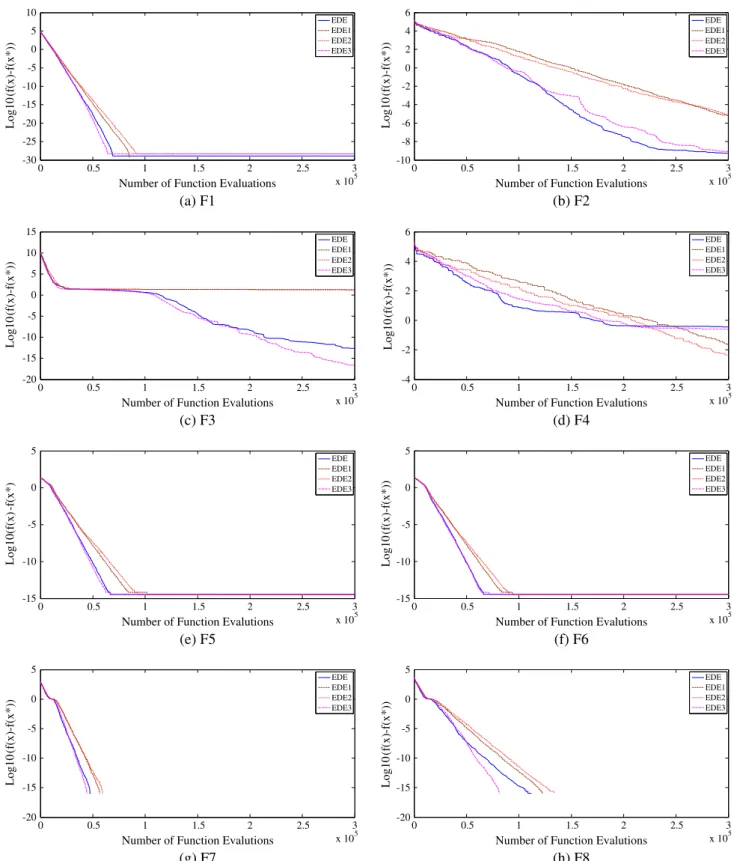
In order to evaluate the final solution quality, efficiency, con-vergence rate, and robustness produced by all algorithms, the performance of the three different versions of EDE algorithm are investigated based on the 30-dimensional functions. The parameters used are fixed as same as those in Section 4.2. The overall comparison results of the EDE algorithm against its ver-sions and conventional DE algorithm are summarized inTable 6. Furthermore, in order to analyze the convergence behavior of each algorithm compared, the convergence characteristics in terms of the best fitness value of the median run of each algo-rithm for functions f1–f14 with dimension 30 is illustrated in

Fig. 2. Indeed, the presented results in Table 6 explain that

EDE and its three different variants obtain better high quality results on unimodal problemf1, multi-modal functionsf5,f6 and composition functionf13. Therefore, it is clearly that the similar performance and common results exhibited by EDE and its versions on these functions is due to the effect of the pro-posed uniform cross over (CR) probability and uniform scaling factor (F). Furthermore, with respect to the remaining func-tions, for the EDE 2 algorithm, it is clearly observed that the incorporation of the random mutation and modified (BGA) mutation to EDE 1 deteriorates performance slightly on func-tions (f3,f7,f9,f10andf11) while deteriorates performance signif-icantly on function f12. However, produces a significant improvement in composition functionf14. Finally, EDE 1 and EDE 2 exhibit the similar performance on functions (f2,f4and f8). Thus, the joining of random mutation and modified (BGA) mutation in EDE 2 has a slight negative influence on the final solution quality and the convergence speed on some

Table 6 Comparison between EDE and EDE with different versions on 30D problems.

Functions EDE1 EDE2 EDE3 EDE

Mean STD Mean STD Mean STD Mean STD

f1 3.28E30 1.22E29 3.36E30 1.30E29 1.06E28 1.01E28 1.60E28 4.63E28

0 0 0 –

f2 9.58E06 1.27E05 1.19E05 1.18E05 3.85E09 8.82E09 2.29E09 4.53E09

1 1 0 –

f3 1.31E+01 7.37E+00 2.07E+01 1.26E+01 5.31E01 1.40E+00 1.85E11 4.56E11

1 1 1 –

f4 7.94E02 1.46E01 1.02E02 1.15E02 5.68E01 7.93E01 1.55E+00 2.97E+00

1 1 1 –

f5 3.55E15 0.00E+00 3.55E15 0.00E+00 3.55E15 0.00E+00 3.55E15 0.00E+00

0 0 0 –

f6 3.55E15 0.00E+00 3.55E15 0.00E+00 3.55E15 0.00E+00 3.55E15 0.00E+00

0 0 0 –

f7 0+00E+00 0+00E+00 1.15E03 3.07E03 6.57E04 2.54E03 1.15E03 3.07E03

1 0 0 –

f8 2.79E03 4.14E03 4.93E04 1.91E03 2.62E03 4.60E03 4.10E03 6.22E03

0 1 0 –

f9 5.72E+01 1.34E+01 9.95E+01 1.72E+01 1.44E+01 5.59E+00 0+00E+00 0+00E+00

1 1 1 –

f10 1.68E+02 7.49E+00 1.81E+02 6.67E+00 5.29E+01 1.53E+01 3.88E+01 7.13E+00

1 1 1 –

f11 5.82E+01 1.17E+01 9.69E+01 1.22E+01 2.06E+1 5.30E+00 0+00E+00 0+00E+00

1 1 1 –

f12 4.38E+00 1.69E+01 1.61E+03 2.09E+03 3.21E+02 2.12E+02 0+00E+00 0+00E+00

1 1 1 –

f13 3.50E32 1.36E31 1.75E32 4.63E32 3.94E31 6.72E31 4.16E31 3.31E31

0 0 0 –

f14 1.57E+00 8.03E01 8.97E01 7.02E01 2.84E+00 1.13E+00 1.98E+00 9.03E01

cases. On the other hand, for the EDE 3 algorithm, it can be seen that by embedding the proposed mutation in EDE 1 algorithm, a significant improvement in the performance of EDE 3 has been detected and achieved on functions (f2–f3andf9–f11). On the contrary, EDE1 algorithm has performed better than EDE3 on problem (f7,f12andf14). Meanwhile, EDE1 and IDE3 exhibit

similar performance on functionsf4andf8. For the EDE algo-rithm, it exhibits substantial performance improvement on functions (f2–f3andf9–f12). Therefore, it can be seen that by embedding the new mutation scheme , random mutation and modified (BGA) mutation together in EDE 1 algorithm, ex-treme and ultimate improvement in the performance of EDE 1

0 0.5 1 1.5 2 2.5 3 x 105 -30 -25 -20 -15 -10 -5 0 5 10

Number of Function Evaluations

Log10 (f(x)-f(x*)) EDE EDE1 EDE2 EDE3 (a) F1 0 0.5 1 1.5 2 2.5 3 x 105 -10 -8 -6 -4 -2 0 2 4 6

Number of Function Evalutions

Log10 (f(x)-f(x*)) EDE EDE1 EDE2 EDE3 (b) F2 0 0.5 1 1.5 2 2.5 3 x 105 -20 -15 -10 -5 0 5 10 15

Number of Function Evalutions

Log10 (f(x)-f(x*)) EDE EDE1 EDE2 EDE3 (c) F3 0 0.5 1 1.5 2 2.5 3 x 105 -4 -2 0 2 4 6

Number of Function Evalutions

Log10 (f(x)-f(x*)) EDE EDE1 EDE2 EDE3 (d) F4 0 0.5 1 1.5 2 2.5 3 x 105 -15 -10 -5 0 5

Number of Function Evalutions

Log10(f(x) -f(x*) EDE EDE1 EDE2 EDE3 (e) F5 0 0.5 1 1.5 2 2.5 3 x 105 -15 -10 -5 0 5

Number of Function Evalutions

Log10 (f(x)-f(x*)) EDE EDE1 EDE2 EDE3 (f) F6 0 0.5 1 1.5 2 2.5 3 x 105 -20 -15 -10 -5 0 5

Number of Function Evalutions

Log10 (f(x)-f(x*)) EDE EDE1 EDE2 EDE3 (g) F7 0 0.5 1 1.5 2 2.5 3 x 105 -20 -15 -10 -5 0 5

Number of Function Evalutions

Log10 (f(x)-f(x*)) EDE EDE1 EDE2 EDE3 (h) F8

has been detected and achieved on these functions. Moreover, from thet-test results, it can be observed that EDE is inferior to, equal to, superior to its compared versions in 6, 18 and 18 cases out of the total 42 cases, respectively. Consequently, EDE algorithm is always either better or equal. Overall, it can be concluded that the performance of the EDE is superior to and/or competitive with EDE 1, EDE 2 and EDE 3 algorithms in terms of final solution quality, stability and robustness. Addi-tionally, as previously mentioned, the convergence graph in

Fig. 2illustrate that EDE 3 and EDE algorithms converge to

better or global solution faster than EDE 1 and IDE 2 in all cases with exception to functionsf4andf14where EDE 2 converges faster than all compared algorithms. However, EDE algorithm converges faster than EDE 3 on functions (f9,f11andf12) while EDE slightly slower than EDE1 and DE 2 on functionf4. It is clear that the proposed modifications play a vital role and has a significant impact in improving the convergence speed of EDE algorithm for most problems. The EDE algorithm has a considerable ability to maintain its convergence rate, improve

its diversity as well as advance its local tendency through a search process. Thus, after the above analysis and discussion, the proposed algorithm EDE show competitive performance in terms of quality of solution, efficiency, convergence rate and robustness. It is superior to conventional DE methods, and it is also competitive with and, in some cases superior to the-state-of-the-art well-known self-adaptive DE algorithms and its three versions EDE 1, EDE 2 and EDE 3. Accordingly, the main benefits of the proposed modifications are the remark-able balance between the exploration capability and exploita-tion tendency through the optimizaexploita-tion process that leads to superior performance with fast convergence speed and the ex-treme robustness over the entire range of benchmark functions which are the weak points of all evolutionary algorithms. 6. Conclusion and future works

In this paper, an Effective Differential Evolution (EDE) algo-rithm is presented for solving unconstrained global

real-param-0 0.5 1 1.5 2 2.5 3 x 105 1.5 2 2.5 3

Number of Function Evaltions

Log10 (f(x)-f(x*)) EDE EDE1 EDE2 EDE3 (j) F10 0 0.5 1 1.5 2 2.5 3 x 105 -15 -10 -5 0 5 10

Number of Function Evalutions

Lo10(f(x)-f(x*)) EDE EDE1 EDE2 EDE3 (k) F11 0 0.5 1 1.5 2 2.5 3 x 105 -15 -10 -5 0 5

Number of Function Evalutions

Log10 (f(x)-f(x*)) EDE EDE2 EDE2 EDE3 (i) F9 0 0.5 1 1.5 2 2.5 3 x 105 -15 -10 -5 0 5

Number of Function Evalutions

Log10 (f(x)-f(*)) EDE EDE1 EDE2 EDE3 (l) F12 0 0.5 1 1.5 2 2.5 3 x 105 -35 -30 -25 -20 -15 -10 -5 0 5

Number of Function Evalutions

Log10 (f(x)-f(*)) EDE EDE1 EDE2 EDE3 (m) F13 0 0.5 1 1.5 2 2.5 3 x 105 -0.5 0 0.5 1 1.5 2 2.5 3 3.5

Number of Function Evalutions

Log10 (f(x)-f(x*)) EDE EDE1 EDE2 EDE3 (n) F14 Figure 2 (continued)

eter optimization problems over continuous domain. In order to enhance the local search ability and advance the convergence rate, a new directed mutation rule was presented and it is com-bined with the basic mutation strategy through a linear decreas-ing probability rule. The proposed mutation rule is shown to enhance the local search capabilities of the basic DE and to in-crease the convergence speed. A new scaling factor is intro-duced as uniform random number to enrich the search behavior. Furthermore, a random mutation scheme and a mod-ified Breeder Genetic Algorithm (BGA) mutation scheme are merged to avoid stagnation and/or premature convergence. Additionally, the scaling factor and crossover of DE are intro-duced as uniform random numbers to enrich the search behav-ior and to enhance the diversity of the population. The proposed EDE algorithm has been compared with seven classi-cal DE methods and six recent state-of-the-art parameter adap-tive differential evolution variants over a suite of 14 bound constrained numerical optimization problems. The experimen-tal results and comparisons have shown that the EDE algo-rithm performs better in unconstrained optimization problems with different types, complexity and dimensionality; it performs better with regard to the search process efficiency, the final solution quality, the convergence rate, and robustness, when compared with other algorithms. Finally, the perfor-mance of the EDE algorithm is statistically superior to and con-ventional DE algorithms and it is competitive with other recent well-known self-adaptive DE algorithms especially with high dimensions problems. The effectiveness and benefits of the pro-posed modifications used in EDE have been experimentally investigated and compared. It is found that the proposed algo-rithm EDE shows competitive performance in terms of quality of solution, efficiency, convergence rate and robustness. It is statistically superior to and competitive with its three versions EDE1, EDE 2 and EDE 3 basically based on DE/rand/1/bin strategy. Several current and future works can be developed from this study. Firstly, Current research efforts focus on how to modify the EDE algorithm for handling constrained and multi-objective optimization problems as well as to solve practical engineering optimization problems and real world applications. Secondly, it would be very interesting to propose a self-adaptive EDE version. However, Future works may fo-cus on applying the algorithm to solve standard benchmark functions and high dimensions or large scale global optimiza-tion problems and compare the results with the most recent algorithms.

References

[1] Storn R, Price K. Differential evolution-a simple and efficient adaptive scheme for global optimization over continuous spaces. Technical report TR-95-012, ICSI; 1995. < http://.icsi.berke-ley.edu/~storn/litera.html>.

[2] Storn R, Price K. Differential evolution – a simple and efficient heuristic for global optimization over continuous spaces. J Global Optim 1997;11(4):341–59.

[3] Price K, Storn R, Lampinen J. Differential evolution: a practical approach to global optimization. Heidelberg: Springer; 2005.

[4] Pan QK, Wang L, Gao L, Li WD. An effective hybrid discrete differential evolution algorithm for the flow shop scheduling with intermediate buffers. Inf Sci 2011;181(3):668–85.

[5] Omran M, Engelbrecht AP, Salman A. Differential evolution methods for unsupervised image classification. In: Proceedings of

IEEE congress on evolutionary computation, vol. 2; 2005. p. 966– 73.

[6] Hachicha N, Jarboui B, Siarry P. A fuzzy logic control using a differential evolution algorithm aimed at modeling the financial market dynamics. Inf Sci 2011;181(1):79–91.

[7] Das S, Abraham A, Konar A. Automatic clustering using an improved differential evolution algorithm. IEEE Trans Syst Man Cybern – Part A: Syst Hum 2008;38(1):218–37.

[8] Das S, Konar A. Two-dimensional IIR filter design with modern search heuristics: a comparative study. Int J Comput Intell Appl 2006;6(3):329–55.

[9] Das S, Sil S. Kernel-induced fuzzy clustering of image pixels with an improved differential evolution algorithm. Inf Sci 2010;180(8):1237–56.

[10] Wang Y, Li B, Weise T. Estimation of distribution and differential evolution cooperation for large scale economic load dispatch optimization of power systems. Inf Sci 2010;180(12):2405–20. [11] Aliev AR, Pedrycz W, Guirimov BG, Aliev RR, Ilhan U, Babagil

M, Mammadli S. Type-2 fuzzy neural networks with fuzzy clustering and differential evolution optimization. Inf Sci 2011;181(9):1591–608.

[12] Noman N, Iba H. Accelerating differential evolution using an adaptive local search. IEEE Trans Evol Comput 2008;12(1):107–25.

[13] Das S, Abraham A, Chakraborty UK, Konar A. Differential evolution using a neighborhood based mutation operator. IEEE Trans Evol Comput 2009;13(3):526–53.

[14] Lampinen J, Zelinka I. On stagnation of the differential evolution algorithm. In: Matousˇek R, Osˇmera P, editors. Proceedings of Mendel 2000, 6th international conference on soft computing; 2000. p. 76–83.

[15] Ga¨mperle R, Mu¨ller SD, Koumoutsakos P. A parameter study for differential evolution. In: Grmela A, Mastorakis NE, editors. Advances in intelligent systems, fuzzy systems, evolutionary computation. Interlaken, Switzerland: WSEAS Press; 2002. p. 293–8.

[16] Ro¨nkko¨nen J, Kukkonen S, Price KV. Real-parameter optimiza-tion with differential evoluoptimiza-tion. In: Proceedings of IEEE congress on evolutionary computation, IEEE Computer Society, Washing-ton, DC, vol. 1; 2005. p. 506–13.

[17] Liu J, Lampinen J. A fuzzy adaptive differential evolution algorithm. Soft Comput 2005;9(6):448–62.

[18] Brest J, Greiner S, Bosˇkovic´ B, Mernik M, zˇumer V. Self-adapting control parameters in differential evolution: a comparative study on numerical benchmark problems. IEEE Trans Evol Comput 2006;10(6):646–57.

[19] Omran MGH, Salman A, Engelbrecht AP. Self-adaptive differ-ential evolution. In: Computational intelligence and security, PT 1, proceedings, lecture notes in artificial intelligence; 2005. p. 192– 99.

[20] Zaharie D. Control of population diversity and adaptation in differential evolution algorithms. In: Matousek R, Osmera P, editors. Proceedings of Mendel 2003, 9th international conference on soft computing; 2003. p. 41–6.

[21] Ali MM, To¨rn A. Population set based global optimization algorithms: some modifications and numerical studies. Comput Oper Res 2004;31:1703–25.

[22] Neri F, Tirronen V. Scale factor local search in differential evolution. Memetic Comput J 2009;1(2):153–71.

[23] Qin AK, Huang VL, Suganthan PN. Differential evolution algorithm with strategy adaptation for global numerical optimi-zation. IEEE Trans Evol Comput 2009;13(2):398–417.

[24] Zhang JQ, Sanderson AC. JADE: adaptive differential evolution with optional external archive. IEEE Trans Evol Comput 2009;13(5):945–58.

[25] Ghosh A, Das S, Chowdhury A, Giri R. An improved differential evolution algorithm with fitness-based adaptation of the control parameters. Inf Sci 2011;181(18):3749–65.

[26] Fan HY, Lampinen J. A trigonometric mutation approach to differential evolution. J Global Optim 2003;27(1):105–29. [27] Mohamed AW, Sabry HZ. Constrained optimization based on

modified differential evolution algorithm. Inf Sci 2012;194:171–208.

[28] Mohamed AW, Sabry HZ, Khorshid M. An alternative differen-tial evolution algorithm for global optimization. J Adv Res 2012;3(2):149–65.

[29] Kaelo P, Ali MM. A numerical study of some modified differ-ential evolution. Eur J Oper Res 2006;196(3):1176–84.

[30] Liu G, Li Y, Nie X, Zheng H. A novel clustering-based differential evolution with 2 multi-parent crossovers for global optimization. Appl Soft Comput 2012;12(2):663–81.

[31] Ali M, Siarry P, Pant M. An efficient Differential Evolution based algorithm for solving multi-objective optimization problems. Eur J Oper Res 2012;217(2):404–16.

[32] Triguero I, Derrac J, Garci S, Herrera F. Integrating a differential evolution feature weighting scheme into prototype generation. Neurocomputing 2012;97:332–43.

[33] Ali M, Pant M, Abraham A. Improving differential evolution algorithm by synergizing different improvement mechanisms. ACM Trans Auton Adapt Syst 2012;7(2):1–32.

[34] Islam SM, Das S, Ghosh S, Roy S, Suganthan PN. An adaptive differential evolution algorithm with novel mutation and cross-over strategies for global numerical optimization. IEEE Trans Syst Man Cybern Part B: Cybern 2012;42(2):482–500.

[35] Mallipeddi R, Suganthan PN, Pan QK, Tasgetiren MF. Differ-ential evolution algorithm with ensemble of parameters and mutation strategies. Appl Soft Comput 2011;11(2):1679–96. [36] Das S S, Suganthan PN. Differential evolution: a survey of the

state-of-the-art. IEEE Trans Evol Comput 2011;15(1):4–31. [37] Xu Y, Wang L, Li L. An effective hybrid algorithm based on

simplex search and differential evolution for global optimization. Int Conf Intell Comput 2009:341–50.

[38] Feoktistov V. Differential evolution: in search of solutions. Berlin, Germany: Springer-Verlag; 2006.

[39] Mu¨hlenbein H, Voosen DS. Predictive models for the breeder genetic algorithm – I. Continuous parameter optimization. Evol Comput 1993;1(1):25–49.

[40] Liang JJ, Suganthan PN, Deb K. Novel composition test functions for numerical global optimization. In: Proceedings of IEEE Swarm intelligence symposium, Pasadena, CA; 2005. p. 68– 75.

[41] Shang YW, Qiu YH. A note on the extended rosenbrock function. Evol Comput 2006;14(1):119–26.

[42] Derrac J, Garcı´a S, Molina D, Herrera F. A practical tutorial on the use of nonparametric statistical tests as a methodology for comparing evolutionary and swarm intelligence algorithms. Swarm Evol Comput 2011;1(1):3–18.

[43] Eiben AE, Smit SK. Parameter tuning for configuring and analyzing evolutionary algorithms. Swarm Evol Comput 2011;1(1):19–31.