A case study of material testing for corrosion in low temperature geothermal systems

(1)

A CASE STUDY OF MATERIAL TESTING

FOR CORROSION

IN LOW TEMPERATURE GEOTHERMAL

SYSTEMS

A Thesis submitted to

the Graduate School of Engineering and Science of

Izmir Institute of Technology

in Partial Fulfillment of the Requirements for the Degree of

MASTER OF SCIENCE

in Materials Science and Engineering

by

Umut NCE

July, 2005

Izmir, Turkey

(2)

We approve the thesis of Umut NCE

Date of Signature

... 25 July 2005 Assoc. Prof. Dr. Mustafa GÜDEN

Supervisor

Department of Mechanical Engineering Izmir Institute of Technology

... 25 July 2005 Prof. Dr. Macit TOKSOY

Co-Supervisor

... 25 July 2005 Prof. Dr. Muhsin Ç FTÇ O LU

Department of Material Science and Engineering Izmir Institute of Technology

... 25 July 2005 Prof. Dr. Zafer LKEN

... 25 July 2005 Assoc. Prof. Dr. Sedat AKKURT

... 25 July 2005 Prof. Dr. Muhsin Ç FTÇ O LU

Head of Department

Izmir Institute of Technology

...

Assoc. Prof. Dr. Semahat Özdemir

(3)

ACKNOWLEDGEMENTS

I would like to express my gratitude to my advisor Assoc. Prof. Dr. Mustafa Güden and my co-advisor Prof. Dr. Macit Toksoy for their invaluable advice, guidance, and encouragement.

I would like to thank to Izmir-Balçova geothermal Inc. staff for supporting throughout my M. Sc. studies. I also thank to Fasih Kutluay, Furkan E refgil and Demir Ba e mez for their contributions to this study.

Thanks are also extended to Izmir institute of technology machine shop staff who helped to start-up and use wire-spark erosion machine.

I would like to thank the Center for Materials Research staff at Izmir Institute of Technology for their help and patience during my study.

I would also like to thank my friends Ece Yapa an, Sinan Kapçak and Levent Aydın and my colleague for their encouragement, help and patience.

I am also grateful to my parents for their endless support during my thesis and all of my life.

(4)

ABSTRACT

The main goal of this study is to determine the corrosion rate and mechanisms of an St-37 steel material currently used as a pipeline material in Izmir–Balçova Geothermal District Heating System. Alternative steel piping materials, AISI 304, AISI 316, AISI 316L austenitic stainless steels, were also investigated for their corrosion behaviour in the same geothermal system. Two fluid velocities, 0.02 and 9.6 m/s, showing the low or stagnant and high velocity fluid flow respectively were selected for the corrosion experiments at the site. Intentionally prepared tensile St-37 test specimens were used to investigate the effect of corrosion (particularly pitting type of corrosion) on the ultimate tensile strength of the steel, while conventional test coupons were used in the testing of stainless steels. These tests were further accompanied by the qualitative laboratory tests involving Ryznar stability index and electropotential measurements. It was found that laboratory measurements, Ryznar stability index, pitting resistance equivalent and electropotential measurements showed good agreement with the result of corrosion experiments conducted at the site. Although the uniform corrosion rates were relatively low in the tested steels, the pitting corrosion rate was greatly promoted in St-37 samples at the low fluid velocity, mainly driven by the SRB activity and tubercle formation. The tensile tests on the St-37 corroded samples have further shown that the UTS decreased as the exposure time increased. The decrease in the UTS of St-37 was more pronounced in the samples tested at the lower fluid velocity, which showed a good agreement with the measured maximum pitting depths found in these samples. The service life time of the St-37 was further predicted for two selected fluid velocities using the equations developed for the effect of defects on the bursting pressure of the pipelines. The predicted service life of St-37 was 57 and 95 months for low and high velocity fluid flow respectively. These service lives were also comparable with the reported service life of the pipelines used in the studied geothermal system. Finally, a solution were proposed to increase the service lifetime of St-37 pipes: addition of SRB activity reducing reagents to the fluid.

(5)

ÖZ

Bu çalı mada Izmir-Balçova bölgesel jeotermal ısıtma sisteminde yaygın ekilde boru malzemesi olarak kullanılan St-37 çeli iyle alternatif AISI 304, 316, 316L östenitik paslanmaz çeliklerin ortalama özelliklere sahip bir jeotermal kuyu içerisindeki korozyon davranı ı ve korozyon hızları 0.02 m/s ve 9.6 m/s akı kan hızlarında belirlenmi tir. Korozyona u ramı çeli in mekaniksel özelliklerindeki de i imini incelemek ve boru hatlarının sistemdeki ömürlerini saptamak amacıyla St-37 çeli i korozyon testi numuneleri çekme deneyi numunesi biçiminde yapılmı tır. Paslanmaz çelik numuneleri ise korozyon deneylerinde sıklıkla kullanılan biçim ve boyutta, dikdörtgen olarak ekillendirilmi tir. Öncelikle yapılan Ryznar indeksi, çukurcuk korozyonu dayanım denklemi hesaplamaları ve elekto-potensiyel ölçümleri ile tahmin edilen korozyon davranı ları ve yapılan niteliksel kar ıla tırmaların uzun süreli saha deneyleriyle büyük ölçüde uyumluluk gösterdi i gözlenmi tir. Uzun süreli saha deneyleri; bütün çeliklerin dü ük homojen da ılımlı korozyon hızlarına sahip oldu unu gösterirken, özellikle dü ük akı kan hızında maruz bırakılmı St-37 çeli i için sulfat indirgeyici bakteriler ve “tubercle” olarak adlandırılan olu umlar tarafından tetiklenen çukurcuk korozyonun çok daha hızlı ilerledi i tespit edilmi tir. Yapılan çekme deneyi sonuçları St-37 çeli inin maksimum çekme gerilmesinin artan maruz kalma zamanı için azaldı ını göstermi tir. Bu durumun St-37 çeli inin yüzeyinde tespit edilen maksimum çukurcuk derinli inin artan maruz kalma zamanı için artması ile önemli ölçüde uyumluluk gösterdi i tespit edilmi tir. Boru hatlarının patlama basınçlarının hesaplanması için geli tirilmi olan formulasyonlar ile St-37 çeli inden yapılmı boru hatlarının dü ük akı kan hızında 57 ay ve yüksek akı kan hızında 95 ay olarak tahmin edilen ömürlerinin incelenen kuyuda kullanılan boru hatlarının ömürleriyle kar ıla tırılabilir ölçüde do ru oldu u görülmü tür. Sonuç olarak boru hatlarının ömrünün arttırılması için sulfat indirgeyici bakterilerin aktivasyonunu önlemek veya indirgemek için kimyasal kullanımı önerilmi tir.

(6)

LIST OF FIGURES

Figure 1.1. Change on worldwide energy use

and growth in fossil fuel consumptions ...2

Figure 1.2. Change on growth in CO2 in the atmosphere with years and CO2 emissions from energy consumption for electricity generation ...2

Figure 1.3. Temperatures in Earth and layer of the Earth ...3

Figure 1.4. Schematic representation of an ideal geothermal system ...4

Figure 1.5. A sample of district heating system...5

Figure 1.6. Chemical content of geothermal fluid and their average concentrations...8

Figure 1.7. Schematic representation of carbonic chain ...10

Figure 1.8. Stainless steel pipe scaling layer section ...11

Figure 2.1. The corrosion cycle of steel ...15

Figure 2.2. Reversible cell containing iron and zinc in equilibrium with their ions ...20

Figure 2.3. Standart half-cell electrode potentials vs. normal hydrogen electrode at 25 0C...21

Figure 2.4. Potential-pH diagram for water...22

Figure 2.5. Thermodynamic boundaries of the types of corrosion observed on steel and E-pH ranges for water environments ...23

Figure 2.6. (a) E-pH diagram of iron in water at 25 0C, (b)E-pH diagram of iron in water 85 0C ...23

Figure 2.7. Solubility of oxygen in water in equilibrium with air at different temperatures...24

Figure 2.8. Schematic representation of corrosion of iron in hydrochloric acid ...25

Figure 2.9. Effect of water velocity on corrosion of carbon steel. (a) Distilled water +10 ppm Cl- , 50 0C, 14 days. (b) Soft tap water, Tokyo, Japan, room temperature, 67 days. (c) Soft tap water, Amagasaki, Japan, 20 0C, 15 days (killed steel). (d) Soft tap water, Amagasaki, Japan, 20 0C, 15 days (rimmed steel) ...29

(9)

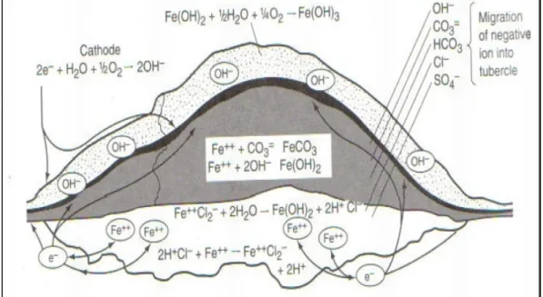
Figure 2.10. (I)- Effect of water velocity and chloride concentrations

on corrosion of carbon steel. Distilled water+NaCl, 50 0C, 14 days ...30 Figure 2.11. Most observed pit shapes ...31 Figure 2.12. Pits on the surface of a stainless heat exchanger...33 Figure 2.13. Schematic of tubercle structures formed

on steel in oxygenated waters ...34 Figure 2.14. Chloride required to produce localized corrosion

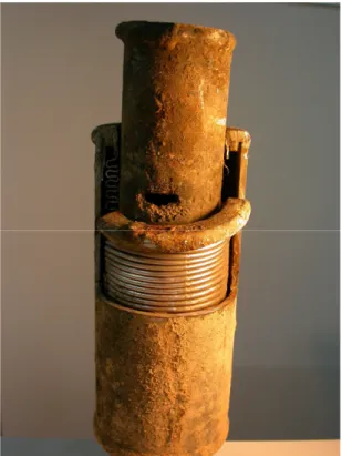
of type 304-316 stainless steels as a function of temperature...36 Figure 2.15. Corrosion caused by the galvanic effect on a

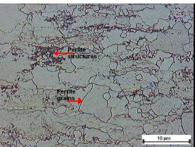
compensators taken from Balçova-Izmir geothermal system ...38 Figure 3.1. The optical micrograh of the microstructure

of St-37 steel, showing feritte grains and fine perlitic structure ...44 Figure 3.2. The optical micrograh of the microstructure

of AISI 304 austenitic stainless steels,

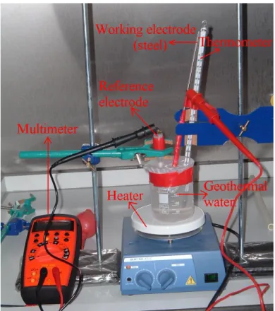
showing austenite grains and twins...44 Figure 3.3. Experimental set-up used to measure electropotential

of the steels tested in the actual geothermal water...45 Figure 3.4. The Reference electrodes conversion chart...46 Figure 3.5. St-37 steel tensile test specimen machined

according to ASTM E-8 and dimensions...47 Figure 3.6. Austenitic stainless steel corrosion test coupons...47 Figure 3.7. Schematic representation of experimental set-up...48 Figure 3.8. Schematic of St-37 specimens replacement

in section A using heat resistant ropes ...49 Figure 3.9.(a) temperature, (b) pH, (c) electrical conductivity and

(d) chloride content of the few wells in Izmir-Balçova

district heating geothermal system...50 Figure 4.1. Prediction of investigated steel corrosion types

in thermodynamic boundaries of the types of corrosion

observed on steel and E-pH ranges for water environments graph...55 Figure 4.2. Weight loss and corrosion rate vs. exposure time

for st-37 at a fluid velocity of 0.02 m/s...57 Figure 4.3. SEM surface images of the specimen surfaces

(10)

Figure 4.4. The EDX analyses of the corrosion products

after exposure times of (a) 336, (b) 845 and (c) 1207 h...59 Figure 4.5. An SEM image showing corroded (A) and uncorroded

(B) sites on an St-37 sample surface after 336 h exposure ...60 Figure 4.6. The EDX analyses results of the specimen surfaces

shown in Figure 4.5, (a) site A and (b) site B ...61 Figure 4.7. The epoxy-mounted and polished cross-section

SEM image of an St-37 sample (336 h),

showing the split corrosion layers marked as A and B ...62 Figure 4.8. The EDX analyses results of the cross-section

shown in Figure 4.7, (a) section A and (b) section B...62

Figure 4.9.The EDX line scans of Sb, S and Fe through

the corrosion layer (336 h exposure)...63 Figure 4.10. The epoxy-mounted and polished cross-section

SEM image of an St-37 sample (845 h), showing

split corrosion layers marked as A and B ...63 Figure 4.11. EDX analysis results of the cross-sections shown

in Figure 4.10, (a) section A and (b) section B...64 Figure 4.12. EDX line scans of Sb, Fe and S through

the corrosion layer (after 845 h exposure) ...65 Figure 4.13. SEM image of a pit, showing the anodic

and cathodic zones and the accumulation

of the SRB in the anodic zone...66 Figure 4.14. SEM images of the SRB inside the pits after

(a) 336 h and (b) 1207 h exposure ...66 Figure 4.15. (a) SEM image of a tubercle structure of porous

columnar fibers formed on the corroded St-37 steel surface

and (b) EDX analysis of the outer crust...67 Figure 4.16. Stereo zoom microscope images of

(a) a tubercle structure and (b) pitting corrosion initiated

under the tubercle structure...68 Figure 4.17. Stereo zoom microscope images of

(a) a tubercle structure and (b) pitting corrosion

(11)

Figure 4.18. Typical XRD analysis of the corrosion products form on the surface of St-37 samples after

336, 845 and 1207 h exposure ...69 Figure 4.19. Stereo zoom microscope images of the pits

formed on surfaces of St-37 steel at increasing exposure times ...71 Figure 4.20. The maximum pit depths of 1581 h exposed specimens...71 Figure 4.21. Maximum pit depth and thickness loss as

function exposure time at 0.02 m/s fluid velocity...72

Figure 4.22. Maximum pitting corrosion rates vs. exposure time

of St-37 steel at 0.02 m/s fluid velocity ...72 Figure 4.23. Stress-strain curves of St-37 carbon steel specimens

for increasing exposure times ...74 Figure 4.24. UTS vs. exposure time...74 Figure 4.25. The variation of UTS values of the specimens

(a) uncorroded and (b) exposed 1581 h ...75 Figure 4.26. Bursting Pressure vs. service time of St-steel

at low velocity fluid flow based on

DnV 1996, Norway standarts (Eqn. 3.8)...75 Figure 4.27. Bursting Pressure vs. service time of St-steel

at low velocity fluid flow based on the Eqn. 3.9...76 Figure 4.28. Weight loss and corrosion rate vs. exposure time

for st-37 at fluid velocity of 9.6 m/s...77 Figure 4.29. SEM surface images of specimen after

exposure times of (a) 336, (b) 802 and (c) 336 h ...78 Figure 4.30. EDX analyses of corrosion products at exposure times

of (a) 336 and (b) 802 h ...79 Figure 4.31. The epoxy-mounted and polished cross-section

SEM image of an St-37 sample (336 h), showing the

split corrosion layers marked as A, B, C and D...80 Figure 4.32. EDX analyses results of the cross-sections

shown in Figure 4.31, regions: (a) A, (b) B, (c) C and (d) D...81 Figure 4.33. The epoxy-mounted and polished cross-section

(12)

Figure 4.34. EDX analyses results of the cross-sections shown

in Figure 4.32, (a) section A and (b) section B...83 Figure 4.35. SEM image of a sulphate reducing bacterium...83 Figure 4.36. Typical XRD analysis of the corrosion

products after 336 and 802 h exposure ...84 Figure 4.37. Stereo zoom microscope images of the pits

formed on surfaces of St-37 steel at increasing exposure times ...85 Figure 4.38. Maximum pit depth and thickness loss of specimens

as function exposure time at 9.6 m/s fluid velocity ...86 Figure 4.39. Maximum pitting corrosion rates vs. exposure time of St-37

steel at 9.6 m/s fluid velocity ...86 Figure 4.40. Stress-strain graphs of st-37 carbon steel specimens of

increasing exposure time exposed to 9.6 m/s fluid velocity ...87 Figure 4.41. UTS vs. exposure time in samples exposed

to high velocity of fluid...88 Figure 4.42. Bursting Pressure vs. service time of St-37

steel at high velocity fluid flow based

on DnV 1996, Norway standards (Eqn. 3.8)...88 Figure 4.43. Bursting Pressure vs. service time of St-37

steel at high velocity fluid flow based on the Eqn. 3.9 ...89 Figure 4.44. Corrosion rate vs. exposure time

of stainless steels specimens tested at 0.02m/s fluid velocity...90 Figure 4.45. Corrosion rate vs. exposure time

of stainless steels specimens tested at 9.6 m/s fluid velocity...90 Figure 4.46. Calcium carbonate scaling on the surfaces

of the AISI 304 austenitic stainless steel after

(a) 648 and (b) 2000 h exposure to 0.02 m/s fluid velocity...91 Figure 4.47. Calcium carbonate scaling on the surfaces

of the AISI 304 austenitic stainless steel after

(a) 648 and (b) 2000 h exposure to 9.6 m/s fluid velocity...91 Figure 4.48. Stereo zoom microscope images of

(a) aragonite and (b) cubic calcium carbonate precipitation

(13)

Figure 4.49. SEM images of (a) aragonite and (a) cubic calcium carbonate precipitation

on the surface of AISI 304 stainless steel ...92 Figure 4.50. EDX analysis results of aragonite

and cubic calcium carbonate precipitates...92 Figure 4.51. SEM image of SRB accumulation on the surface

of AISI 316 steel at 0,02 m/sn fluid velocity ...93 Figure 4.52. Stereo zoom microscope images of pits

on the AISI 304 austenitic stainless steel surfaces

exposed to 0.02 m/s geothermal water...93 Figure 4.53. SEM images of sulphate reducing bacteria accumulation in pits...94 Figure 4.54. EDX analysis results of pit shown in Figure 4.53

(a) inside and (b) outside of the pit ...94 Figure 4.55. SEM images of calcium carbonate layer

precipitated on (a) AISI 316, (b) AISI 316L stainless steel

surface after 2000 hours exposured time in low fluid velocity...95 Figure 4.56. EDX analysis results of calcium carbonate

(14)

LIST OF TABLES

Table 1.1. Classification of geothermal resources...6

Table 1.2. Analyses of geothermal fluid in B-4 well in Balçova geothermal district heating system ...7

Table 1.3. Principal ions contained in water...8

Table 1.4. Interpretation of the Ryznar stability index ...12

Table 2.1. Iron oxides ...18

Table 2.2. Constants to calculate corrosion rate units desired...28

Table 2.3. Effects of alloying on pitting resistance of stainless steel alloys...33

Table 3.1. Chemical composition of investigated steels...43

Table 3.2. B11 well fluid chemical analysis taken during the exposure of specimens ...51

Table 3.3. The properties of the fluid in the corrosion tests ...51

Table 4.1. EDX analyse results of the tested st-37 specimens at three different exposure times...60

Table 4.2. EDX analyse results of the tested st-37 specimens at two different exposure times...80

Table 4.3. Laboratory and corrosion test results summary (0.02 m/s) ...96

(15)

CHAPTER 1 INTRODUCTION

1.1. Geothermal Energy

“Geothermal” comes from the Greek words of geo (earth) and thermal (heat) and geothermal energy is literally defined as the heat contained within the Earth that generates geological phenomena on a planetary scale. However, “Geothermal energy” is used nowadays to indicate that part of the Earth’s heat that can be recovered and exploited by man. The existence of valcanoes, hot springs, and other thermal phenomena was proved that parts of the interior of the Earth were hot. It was however pointed out that, it was not until a period between sixteenth and seventeenth century, when the first mines were excavated to a few hundred meters below ground level, that man deduced, from simple physical sensations, that the Earth’s temperature increased with depth (Armstead 1983).

Energy resources in the earth can be divided into two groups; fossil fuels and renewable energy resources (EIA 2003, EIA 1994). Geothermal energy, which is an important renewable energy resources, has advantages and disadvantages comparing with other energy sources. World wide energy use increases by year and also with an increase in fossil fuel consumption (Figure 1.1 and Figure 1.2), leading to an increase of

CO2 concentration in the atmosphere. On the contrary, the geothermal energy is

environmentally friendly and leads to lesser amounts of CO2 emmision to the

atmosphere (Figure 1.2). The equivalent savings in the production of CO2 from

electricity generation and direct-use of geothermal systems from fuel oils, natural gas and coal was 89.8, 21.2 and 104.8 millions tons respectively until 1990. Similar numbers were also determined for sulfur oxides as 0, 0.56 and 0.59 million tons for natural gas, fuel oil and coal respectively until 1990 (Goddart 1990). Geothermal energy requires very little land for geothermal power plant that has comparable price to that of fossil-fuel power stations and has less risk than nuclear power plants. Geothermal energy is an limitless source of energy, if it is used in a sustainable way. On the other

(16)

occurred by geothermal water, geothermal systems have very high startup costs, there can be unknown effects on earth’s geologic anomolaus and heated core and not all areas are suitable for geothermal energy.

Figure 1.1. Change on worldwide energy use and growth in fossil fuel consumptions (Nemzer and Carter 2000).

Figure 1.2. Change on growth in CO2 in the atmosphere with years and CO2 emissions

from energy consumption for electricity generation (Nemzer and Carter 2000).

Geothermal heat originates from earth’s fiery consolidation of dust and gas over 4 billion years ago. Calculations showed that the Earth would have cooled and become completely solid without an energy input in addition to that of the sun. It was also proposed that the ultimate source of geothermal energy is radioactive decay within the earth (Bullard 1973). At Earth’s core, 6370 km deep, temperatures may reach over 5000

o_{C (Figure 1.3). The geothermal gradient expresses the increase in temperature with}

depth in the Earth’s crust. The average geothermal gradient was determined to be about

2.5-3 oC per 100 m, down to the depth accesible by drilling with modern technology

(Hochstein 1990). Geothermal systems can therefore be found in regions with a normal or slightly above the normal geothermal gradient. Geothermal systems can be described

(17)

as “convecting water in the upper crust of the Earth, which, in a confined space, transfers heat from a heat source to a heat sink, usually the free surface”.

Figure 1.3. Temperatures in Earth and layer of the Earth (Nemzer and Carter 2000).

A geothermal system may be considered as composing of main elements: a heat source, a reservoir and a fluid. The heat source can be either a very high temperature (>600 0_C)

magmatic intrusion that has reached relatively shallow depths (5-10 km) or, as in low temperature systems, the Earth’s normal temperature increases with depth. The reservoir is a volume of hot permeable rocks and it is covered with impermeable rocks that prevents hot fluids from easily escaping the surface and keep the volume under pressure, see Figure 1.4 as an ideal geothermal system. The fluids are meteoric waters that can penetrate into the Earth’s crust from the recharge areas through hot permeable rocks and can accumulate in reservoir. The fluid may be found as liquid or vapor phase depending on the temperature and pressure and often containes some chemicals and gases. The hot water and/or steam may be extracted by boreholes or, as in the case of springs, escape from the reservoir by natural means. Once, hot water and/or steam travels up to the surface, they can be used in many different types of application (Lindal 1973).

The use of geothermal resources may be divide into three catagories: these are electricity generation, direct-use applications and ground source heat pump applications. The use of geothermal energy for electricity generation was started in 1913 when a power plant of 250kWe was installed in Italy. This development was followed by new power plants installed in New Zealand (1958), Mexico (1959) and United States (1960) (Lund 1999). The geothermal electric and direct-use capacity, and energy use was determined on worldwide based on the papers of 59 countries submitted to the World

(18)

geothermal electric power plants in 21 countries was 7974 MWe and it was predicted that the total installed direct-use plants would increase to a cpacity of 15145 MWe in 58 reporting countries at the end of 2005 (Huttrer 2000).

Figure 1.4. Schematic representation of an ideal geothermal system (Armstead 1983)

According to Hepba lı ve Özgener, there are 11 geothermal district heating systems with a total cpacity of 820 MWt in Turkey (Hepba lı ve Özgener 2003).

Another report gave 992 MWt total capacity of geothermal district heating systems in

Turkey (Merto lu et al. 2000). According to Akku (Akku et al. 2002), the electricity generation and district heating capacity of geothermal systems in Turkey were 764,81 MWe and 1039 MWt, respectively. Electricity generation takes place in conventional

steam turbines and binary plants. Conventional steam turbines operate with a minimum

fluid temperature of 150oC. Atmospheric or condensing exhausts are available for the

conventional steam turbines. The steam, which comes from dry steam wells directly or, comes from wet wells after seperation process, is passed through a turbine and exhausted to the atmosphere by generating electricity. The used geothermal fluid is then reinjected into the reservoir, through an injection well, in order to be reheated, to maintain pressure and to prevent loss of level on geothermal reservoir. The condensing units are more complex and installation costs more expensive while steam consumption is half lesser than atmospheric units. The binary plants utilize secondary working fluids like waste hot waters coming from the seperators. The secondary fluid is used by a

(19)

Rankine cycle where the geothermal fluid yields heat to the secondary fluids via heat exchangers, in which this fluid is heated and vaporized, this vapour is used on a turbine to generate electricity and then cooled and condensed, and the cycle begins again .

Direct heat use is one of the oldest, most verstaile and most common form of the utilization of geothemal energy. Geothermal fluids can be used to grow vegetables, flowers and other crops in green houses. Geothermal fluids can be also used to shorten the time for growing fish, to dry onions and lumber and to wash wool, to pasteurize milk and also space heating of individual buildings and of entire districts, is besides hot spring bathing. In a typical direct-use system, the geothermal fluid is produced from the production borehole, when the geothermal fluid reaches the surface, it is delivered to the application site through the transmission and distrubition system (Figure 1.5).

Figure 1.5. A sample of district heating system (Nemzer and Carter 2000).

In a geothermal direct use system, the geothermal production and disposal systems are coupled, and seperated from the contact by a heat exchanger as depicted schematically in Figure 1.5. The secondary loop is commonly used in large systems to limit the exposure of geothermal fluid to a small potion of the system. In such large systems, there is also a second heat exchanger thet transfers the heat to the building’s heating systems. The fluid in the first loop is injected directly back into re-injection area to be heated and used again after from the contact with the heat exchanger. Geothermal

(20)

few meters below the surface. GHPs are used both for heating or cooling depending on the weather condition. Buildings are heated using the difference between the earth’s temperature and the colder temperature of the air via buried pipelines. In the heating mode, the cold circulating liquid absorbs heat from the ground. This heat is recovered by the heat pump. In the summer, the cooler ground absorbs the surplus heat from houses and buildings more efficiently than the hot air above the ground. Electrical power is used to concentrate heat and move it from one place to another. No any active technology of home cooling is more efficient than the geothermal heat pumps (EIA 1994).

1.2. Definition and Classification of Geothermal Resources

Geothermal resources can be classified based on the enthalpy or temperature of the geothermal fluids. The resources are divided into low, medium and high enthalpy or temperature resources according to several criteria (Table 1.1). Another classification is based on the pressure controlling phase: the liquid-dominated (water –dominated) or vapor-daminated system (White 1973). In liquid-dominated systems, although some vapour may be present, the liquid water is the continuous, pressure controlling phase. Liquid water and vapour are co-exist in the reservoir with vapour continuous, pressure controlling phase in vapour-dominated systems. Geothermal systems can also be classified based on the reservoir equilibrium state (Nicholson 1993). The reservoir is continually recharged by water that is heated and then discharged from the reservoir in the dynamic systems. This category includes low-temperature (<150 0C) and high

temperature systems (>150 0_{C). Heat transfer is occurred by convection and circulation}

of fluid in dynamic systems. There is no recharge or only minor recharges in static systems, which includes low-temperature and geo-pressured systems. Heat is only transferred by conduction in these systems.

Table 1.1. Classification of Geothermal Resources [Muffler 1978, Hochstein 1990]

Classification of Geothermal Resources (a) (b) (c) (d)

Low enthalpy resources - (0C) <90 <125 <100 150

Intermadiate enthalpy resources - (0C) 90-150 125-225 100-200 -

(21)

1.3. Geothermal Fluid Chemistry

The contents of geothermal fluids are composed of gases and liquids. Normal ground waters are usually near neutral in pH and slightly bicarbonate, but they tend to dissolve more sodium chloride and high in salt content when they heated to a relatively

high temperature, very much similar to the geothermal systems. Carbon dioxide (CO2)

and hydogen sulfide (H2S) are the main gases for high temperature systems. Ammonia

(NH3), hydogen (H2), methane (CH4), nitrogen (N2), hydrocarbons (HC), boron (B),

fluorine (F), arsenic (As) and mercury (Hg) may also be present with trace quantities of

oxygen (O2) in low and high temperature systems. The chemicals dissolved in

geothermal fluid at liquid phase include chlorides (Cl), sodium (Na), Magnesium (Mg), potassium (K), fluoride (F), calcium (Ca), silicate (Si), iodine (I), antimony (Sb), strontium (sr), bicarbnonates (HCO3), lithium (Li), arsenic (As), boron (B), hydrogen

sulfide (H2S), mercury (Hg), rubidium (Rb) and ammonia (NH3). Table 1.2 is the

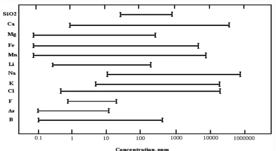
chemical analyses of the geothermal fluid in B-4 well in Balçova (Izmir, Turkey) geothermal district heating system as an representative and the chemical content of geothermal fluid and their avarage concentrations are also shown in Figure 1.6 (Serpen 1999). The chemicals dissolved in geothermal fluid may differ from well to well in the same field because of the geochemistry of the reservoir. However, geothermal fluid commonly contains seven chemical species; these are oxygen, hydrogen ion, chloride ion, sulfide species, carbon dioxide species, ammonia species and sulfide ion. These chemicals have important effect on the corrosion response of materials.

Table 1.2. Analyses of geothermal fluid in B-4 well in Balçova Geothermal District Heating System. T* _{(25) Li}EC + Na+ K+ Mg2+ Ca2+ B SiO2 HCO3- SO42- F- Cl- Name °C pH(25) µS/cm mg/l mg/l mg/l mg/l mg/l mg/l mg/l mg/l mg/l mg/l mg/l B-4 95,7 7,38 1914 1,5 371,4 31,1 12,5 28 8,7 148 634 180 3,9 206

(22)

Figure 1.6. Chemical content of geothermal fluid and their average concentrations

1.4. Scaling Problems Associated with Geothermal Fluid Chemistry

The mineral salts contained in water vary depending on the local geological characteristics and climate. The dissociation of mineral salts produces anions and cations and the most common form of these anions and cations are listed in Table 1.3. The carbonic system is basically derived from the dissolution of carbon dioxide and carbonate minerals in the water. The carbonate system is a weak acid-base system, which exists in aqueous solutions as dissolved carbondioxide (CO2aq), carbonic acid

(H2CO3), bicarbonate (HCO3-), carbonate ions (CO32-) and complexes of these ions such

as CaCO3. Natural water may also contain dissolved gases including oxygen,

carbondioxide and nitrogen and the suspended and colloidal materials such as quartz, organic particles, living organisms and vegetal fragments.

Table 1.3. Principal ions contained in water (Francy et al. 1998)

Cations Anions

Na+ _Sodium _HCO

3- Bicarbonate or Hydrogen carbonate

Mg2+ _Magnesium _CO 32- Carbonate Ca2+ _Calcium _OH- _Hydroxyl K+ _Potassium _Cl- _Chloride Fe2+_{, Fe}3+ _{Ferrous or Ferric} _SO 42- Sulphate H3O+ Hydronium NO3- Nitrate PO43-HPO4 2-H2PO4- Phosphates SiO32- Silicate

(23)

1.4.1. Calcite Scaling

Calcium and carbonates are present in most natural waters and can have potential to form calcium carbonate (CaCO3). The scaling problem is mostly derived

from the destruction of the calco-carbonic balance of the water, leading to the precipitation of calcium carbonate. The change of the parameters such as the pH or

concentration of the dissolved CO2 because of the increase of temperature for example

causes the destruction of calco-carbonic balance. Calcium carbonate precipates from water in one or more of three forms: calcite, arogonite and vaterite. The formation of these allotropes depends on the pressure, temperature, presence of foreign ions and the rate of the precipitation process (Loewental and Marais 1976). The calcite polymorph of calcium carbonate is the most commonly found scale-forming mineral. Vaterite is the solid phase forming first during the precipitation process. At higher temperature, though calcite is the most thermodynamically stable phase, aragonite has been reported to be the first phase to precipitate from the solution (Lippmann 1973). Usually, calcium carbonate precipitates as near cubic crystals of calcite at room temperature or as

needle-like crystals of aragonite at temperatures over 65 oC. The common starting processes of

the precipitation of calcium carbonate are (a) the addition of chemicals resulting in an increase of pH, which allows the dissociation of bicarbonates, (b) degassing or

ventilation, which reduced the concentration of dissolved CO2, thus increasing pH and

(c) increase of the temperature of the water, which makes CO2 less soluble and enables

it to escape by unbalancing the carbonic chain. The carbonic chain process is depicted schematically in Figure 1.7. Carbonate chemistry refers to the series of chemical reactions leading to the equilibria between these reactions. Dissolved carbon dioxide are hydrated according to the following reaction :

CaCO3_aq+H2O⇔CO2,H2O (1.1)

The H2CO3 refers to the composite form, which is the sum of the activities of

molecularly dissolved carbon dioxide CO2aq, and the hydrated form CO2,H2O. The

composite form is convenient due to the analytical difficulties of seperating out CO2aq

from CO2,H2O. The behavior of carbonic system is intimaley involved in the control of

(24)

3 2 3 2 2 3 3 3 3 2 CaCO CO Ca CO H HCO HCO H CO H ⇔ + + ⇔ + ⇔ − + − + − − + (1.2)

Figure 1.7. Schematic representation of carbonic chain (Francy et al. 1998).

The species involved react accordingly to the laws of mass action. When the amount of H2CO3 increases for some reason the equilibrium will move to dissolve the calcium

carbonate. When the quantity of H2CO3 is less than the quantity needed for the

equilibrium then CaCO3 precipates and scaling will occur (Hamrouni and Dhahbi

2002). Moreover; when the solution is heated, CO2 escapes, favoring the bicarbonate

decomposition reaction followed by CaCO3 precipitation by the following reactions

(Web_1 2005) : 3 2 3 2 2 2 3 2 3 ( ) 2 CaCO CO Ca O H CO dissolved CO HCO = + + + = − + − − (1.3)

The composition of the scale in geothermal plants is found to be very complex and depends on many parameters, including the temperature and pressure of the fluid, the history of water-rock relations and the operating conditions. Geothermal systems of low and moderate fluid temperature scale consisting of calcium carbonate as a rule but there are a few exceptions has been remarked untill now. Calcium carbonate scaling

(25)

layer may be in tenths of millimeter in thick as shown in Figure 1.8, which shows a thick scaling layer on a stainless steel taken from Balçova-Izmir geothermal system.

Figure 1.8. Stainless steel pipe scaling layer section

There are numerous methods in use to control scale formation in geothermal systems. Some of the most common measures are the proper design of the geothermal plant and selection of operating conditions, pH adjustment, use of chemical additives and the removal of deposits by chemical or mechanical means. For instance, carbonate deposits can be prevented by the use of scale inhibitors, but the use of inhibitors in preventing sulphide and silica scaling is met by limited success. These scales can be prevented through the decreasing of the pH with the addition of mineral acids. The least desirable method is however the removal of deposits because this technique can be used to clean some specific pieces of equipment like heat exchangers or valves (Andritros et al. 1998). For many years, the Ryznar Index has been used to estimate the corrosivity and scaling tendencies of potable water supplies (Rafferty 1992). However, the statistical study found no significant correlation (at the 95 percent confidence level)

between corrosion and Ryznar Index (Ellis 1985).But this has not been proofed yet for

many different environments and for different types of steels. However, it has been known for many years that indexes can only give a probable indication of the potential corrosivity of a water and generally accepted that if conditions encourage the formation of a protective calcium carbonate film, then corrosion will generally be minimized. Ryznar stability index (RSI) can be used to predict the scale formation and given as (Butlin et al 1951):

(26)

Where, pHs is the pH above which calcium carbonate precipitate. The Ryznar stability

index is interpreted as the indication for the scale formation as tabulated in Table 1.4. It should be noted that the accuracy of the Ryznar stability index is greater as a predictor of scaling than of corrosion.

Table 1.4. Interpretation of the Ryznar Stability Index (Carrier 1965).

RSI-index value Indication

<5.0 Heavy scale

5.0-6.0 Light scale

6.0-7.0 Little scale

7.0-7.5 No scale or Little corrosion

7.5-9.0 Light corrosion

>9.0 Heavy corrosion

Langelier saturation index (LSI) was derived from thermodynamic considerations similar to the Ryznar stability index and used to predict corrosion or scaling tendency of water. It is given with the following relation,

LSI = pH −pH_s (1.5)

The LSI is an equilibrium model and provides an indicator of the degree of saturation of water with respect to calcium carbonate. LSI is probably the most widely used indicator of cooling water scale potential; however it provides no indication of how much scale or calcium carbonate will actually precipate to bring water to equilibrium. In order to

calculate the LSI, it is necessary to know the alkalinity (mg/l as CaCO3) the calcium

hardness (mg/l Ca2+ as CaCO3), the total dissolved solids (mg/l TDS), the actual pH,

and the temperature of water (0_{C). Flentje and by Fujii (Flentje 1961) (Fujii et al. 1983)}

showed that water with a less negative LSI was less corosive. Waters with a slightly negative LSI index may deposit calcium carbonate because of pH fluctuations.

1.4.2. Silica and Carbonate Scaling

Silica and carbonate scales are the ones most extensively studied in connection with geothermal resource utilisation. The precipitated minerals cause ultimately

(27)

problems by restricting the fluid flow, preventing valves from closing, scaling turbine blades etc. Chan reviewed the chemistry of silica deposition and claimed that it was neither simple nor well understood (Chan 1989). Silica deposition depends primarily on the fluid kinetics and it can be delayed from minutes to hours after its saturation limit has been exceeded (Rimstidt and Barnes 1980). The solubility of silica polymorphs with temperature has been studied extensively. Solubilities of various silica polymorphs with temperature have proven useful as geothermometers. Hot water in the reservoir is in equilibrium with quartz and undersaturated with respect to amorphous silica. When a geothermal fluid is brought to the surface, the difference in solubilities between amorphous silica and quartz allows a considerable temperature drop before the solution becomes saturated with respect to amorphous silica. The silica saturation temperature is the temperature at which separated water reaches saturation with respect to amorphous silica. When steam separation takes place above this temperature, then silica scaling usually does not take place and could depend on other dissolved species in the fluid like the fluid salinity. If re-injection is being considered, the temperature is usually kept above the amorphous silica saturation temperature. The pH dependence of silica solubility was also investigated (Henley 1983). Investigations have shown that amorphous silica solubility increased markedly as the pH (temperature) increased. Also, the dissolved salts in geothermal fluid have found appreciable effects on silica solubility. At low salinities, there are no marked effects of dissolved species on silica solubility. But as the concentration of other dissolved species, e.g. NaNO3, MgSO4,

MgCl2, increases in solution the solubility of both quartz and amorphous silica

decreases. In highly concentrated solutions the cation influence on amorphous silica solubility decreases in the following order :

Mg2+ > Ca2+ > Sr2+ > Li+ > Na+ > K+ Anions also have an effect in the order: I- > Br- > Cl- (Kizito 2002)

1.3.3. Metal sulphide and oxide scales.

Criaud and Foulliac (1989) noted the dissolved sulphides of metals such as lead, zinc, copper and iron in geothermal fluids and the utilization schemes and flashing induce deposition of substantial metal sulphide scales. They found that the conditions of

(28)

temperature and salinity in a low-temperature environment such as in sedimentary basins, where bacterial action have occurred, resulted in high concentrations in the fluids. Magnesium silicate scaling was also reported in heating systems. The heating of groundwater depletes the magnesium in the water, and magnesium concentration of geothermal water is mostly below 0.1 mg/kg (Krismannsdottir 1989).

(29)

CHAPTER 2 CORROSION OF STEEL IN WATER : AN OVERVIEW

The word corrode is derived from the latin “corrodore”, which means “ to gnaw to pieces”. Corrosion can be defined in many ways. Some definitions are very narrow and deal with a specific form of corrosion, while others are quite broad and cover many forms of deterioration. As a general definition, corrosion can be defined as a chemical or electrochemical reaction between a material, usually a metal, and its environment that produces a deterioration of the material and its properties. Corrosion is a natural process and all natural processes tend toward the lowest possible energy states. In the case of iron and steel, they have a natural tendency to combine with other chemical elements like water and oxygen to return to their lowest energy states of oxides as illustrated in Figure 2.1 (Davis 2003).

Figure 2.1. The corrosion cycle of steel.

Corrosion can be classified as low temperature and high temperature corrosion or oxidation and electrochemical corrosion or wet and dry corrosion. Wet corrosion occurs when liquid is present. This usually involves aqueous solutions or electrolytes and accounts for the greatest amount of corrosion (Fontana 1987). There are also few

(30)

principal concepts in order to understand basic corrosion phenomena and there are as followings:

• Three possible behavior of a metal when immersed in a solution

• Electrochemical reactions of corrosion

• The many forms of corrosion

2.1 . Three possible behaviors of a metal immersed in a solution

When a metal is exposed to an environment, the metal can behave in three ways. One possibility is that metal can show immunity to the environment. Metals known to display this immunity are called noble metals like gold, silver and platinum. Immune behavior results from the metal being thermodynamically stable in the particular environment; that is, the corrosion reaction does not occur spontaneously. The change

in the free energy (∆G) is a direct measure of the work capacity or maximum electric

energy available from a system. If the change in free energy accompanying the transition of a system from one state to another is negative, this indicates the spontaneous reaction direction of the system, if not, this indicates the immune behavior of the metal to environment. The free-energy change accompanying an electrochemical reaction can be calculated using the following equation.

nFE

G

=

−

∆

(2.1)

Where, n is the number of electrons involved in the reaction, F is the Faraday’s constant, and E is the cell potential.

Another possible behavior is that the metal will corrode, when exposed to the environment. In a specific environment, If the metal corrodes, it is described as active. When active behavior is observed, the metal dissolves in the solution and forms soluble, nonprotective corrosion products. Active corrosion is characterized by the weight loss of the metal. If the metal sample is weighed before and after exposing to the environment, a significant weight loss is measured and thus free energy change is negative. In some cases, although the metal is active, a state of passive behavior is observed. When the metal is immersed into the solution, it corrodes until a thin protective film, also reffered to as a passive film, forms, leading to the slowing down

(31)

the reaction rate to very low levels. All metals and alloys have a thin protective corrosion product film present on their surface resulting from reaction with the environment. For example when an iron or steel is immersed in aqueous environment

hydrous ferrous oxide (FeO.nH2O) or ferrous hydoxide [Fe(OH2)] composes diffusion

barrier layer next to the iron surface through which O2 must diffuse, acting as protective

corrosion layer role on the iron surface. The color of Fe(OH2), although white when the

substance is pure, is normally green to greenish black because of incipient oxidation by air. At the outer surface of protective layer (oxide film), access to dissolved oxygen

converts ferrous oxide to hydrous ferric oxide or ferric hydroxide [Fe(OH3)]. Hydrous

ferric oxide is orange to red-brown in color and makes up most of ordinary rust. It exist as nonmagnetic αFe2O3-hematite or as αFe2O3, the α form having the greater free

energy of formation that means that the greater thermodynamic stability. A magnetic hydous ferrous ferrite, Fe3O4.nH2O, often forms a black intermediate layer between

hydrous Fe2O3 and FeO (Roberge 2000). Important iron-oxides and their colors that are

very important for visual inspection, are listed in Table 2.1 (Cornell and Schewertmann 1996). When a stainless steel is immersed in aqueous environment, for another example, passivity is caused by an ultra-thin surface protective film (1 to 2 nm thick). The passive film on stainless steel has its own composition that is strongly enriched in chromium. When the chromium content is above 10.5% the corrosion product film changes from an active film to a passive film. While the active film continues to grow over the time in the corroding solution until the base metal is consumed, the passive film will form and stop growing. For an alloy containing 15% Cr in its bulk composition, the chromium content in the top layer of passive film can be high as 80%.(Qiu 2002). An interesting observation for the nickel containing stainless steel is that nickel is actually depleted in the passive film and in some cases is found to be enriched in the metallic form immediately beneath the passive film (Cumpson 1993, Seah 1994). The principal constituents of the passive film include metal cations from the substrate with a high

affinity for oxygen. The most common cations are Cr+3_{and Fe}+3_{, although ferrous ions}

Fe+2 are also possible. The cations become associated with water molecules from the surrounding solution. Some of these water molecules lose protons into the solution to

balance the positive charges on the cations by the creation of hydroxyl (OH-) and oxide

(O2-). The passive film on stainless steel is of the “double layers” type, with an inner

(32)

Table 2.1. Iron oxides names, formula and colors (Cornell and Schwertmann 1996).

If such films did not exist on metallic materials exposed to the environment, they would revert back to termodynamically stable condition of their origin as indicated before. The phenomenon of passivity is therefore a critical element controlling corrosion process and usually four conditions are required for breakdown of passive film that initiates localized attack like pitting (Hoar 1967):

1) A certain critical potential must be exceed.

2) Damaging species like chloride or the higher atomic weight halides are needed in the environment to initiate breakdown.

3) An induction time exists, which starts with the initiation of the breakdown process by the introduction of breakdown conditions and ends when the localized corrosion density begins to rise.

4) The presence of highly localized sites where breakdown takes place.

2.1.1 Potential-pH Diagrams

Potential-pH diagrams present a map of the regions of the stability of a metal and its corrosion products in aqueous environments. The diagrams identify conditions under which the metal is stable and will not corrode, soluble reaction products are formed and corrosion will occur and insoluble reaction products are formed and passivity will occur. The diagrams are generated from thermodynamic calculations. These diagrams are also called Pourbaix diagrams in the honor of Marcel Pourbaix, a

(33)

Belgian scientist credited with the development and wide use of these diagrams (Davis 2003). For corrosion in aqueous media, two fundemental variables, namely corrosion potential and pH, are particularly important. Changes in other variables, such as the oxygen concentration, tend to be reflected by changes in the corrosion potential. To draw potential-pH diagrams for an system, it is necessary to determine the potential of a system in which the reactants are not at unit activity like almost all systems, the familiar Nerst equation can be employed for this; that is,

= + (2.2)

where, E is the half-cell potential (V), E0 the standart half-cell potential (V), R is the gas

constant (8.314 j.mol-1.K-1), T is absolute temperature (K), n is the number of electrons transferred, F is the Faraday constant (96487 C.mol-1), aoxid and ared are the

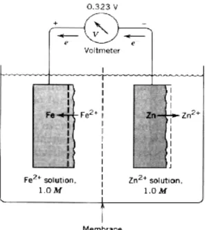
concentrations of oxidized and reduced species. Half-cell potential is not only used for drawing potential-pH diagrams, it is also used to calculate free-energy change for a system. As seen Nerst equation, standart haf-cell potential must be determined in order to calculate half-cell potential. In order to understand how an standart half-cell potential can be determined for example for an zinc and iron system, it can be constructed an electrochemical cell containing iron and zinc electrodes in equilibrium with their ions at

25 0C seperated by a porous membrane to retard mixing, as illustrated in Figure 2.2. For

purposes of simlicity, the concentrations of metal ions are maintained at unit activity; each solution contains 1 gram-atomic weight of metal ion per liter. These reactions will occur in that system for each cell;

Zn =Zn2+_{+2e ; Fe}2+_+2e=Fe

The reaction rates of metal dissolution and deposition in each cell must be the same; there is no net change in the system. These electrodes are called half-cell, and when the concentarions of all reactants are maintained at unit activity, they are termed standart half-cells. If a high-resistance voltmeter is connected to between the iron and zinc electrodes, a potential difference of appriximately 0.323 volts is measured. This is the cell potential that is used in determining free energy of the overall electrochemical reactions (Fontana 1987).

(34)

Figure 2.2. Reversible cell containing iron and zinc in equilibrium with their ions.

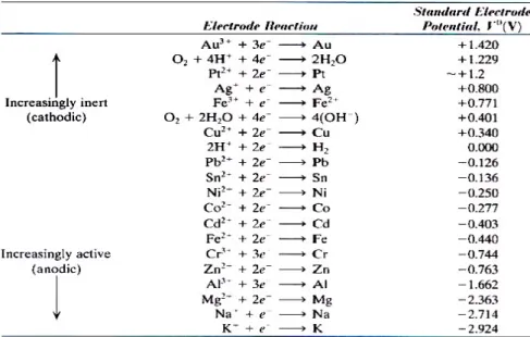
If a platinum inert electrode was used in 1M solution of H+ instead of zinc electrode,

standart half-cell potential would has been read at voltmeter as –0.440 volt for iron. Standart half-cell potentials are referenced against the hydogen electode, which is arbitrarily defined zero like platinum electrode are given Figure 2.3 for the 25 0C electrolyte temperature.

Figure 2.4 shows the potential-pH diagram of water with no metal involved. In between the two diagonal lines marked as a and b in this figure is the region of the stability of water as a function of potential and pH. At any conditions of potential and

pH below the line a, water is thermodynamically unstable with respect to the generation

of hydrogen gas and at any conditions of potential and pH above line b, water is thermodynamically unstable with respect to the evolution of oxygen. For potential and pH conditions between lines a and b, water is thermodynamically stable. Line a

represents the equilibrium for the reaction of hydrogen ions to evolve hydogen gas as, 2

2

2H++ e− →H

The electropotential of above reaction using the Nerst equation is ;

E=0.00−0.059pH (2.3)

The potential at pH=0 is 0 V, and the potential decreses by 0.059V for each unit increase in pH. At any potential and pH below this line, the hydrogen ion in water will react with electrons to evolve hydrogen gas.

(35)

Figure 2.3. Standart half-cell electrode potentials vs. normal hydrogen electrode at 25

o_C.

Figure 2.4. Potential-pH diagram for water (Davis 2003).

Line b represents the equilibrium of oxygen plus hydrogen ions and electrons to form

water as, O H e H O₂+4 ++4 − → ₂

The equation for electropotential is,

pH E=1.229−0.059

(36)

When pH=0, the potential is +1.229 V as seen Figure 2.3 and it decreases by 0.059 V for every unit increase in pH. Above the line b the oxidized species are stable, and water under those conditions reacts spontaneously to produce oxygen and hydrogen ions.

Thus, if a metal electrode is at a potential and pH below line a, hydrogen bubbles will

evolve on the metal surface and similarly, for any metalelectrode potential-pH conditions above line b, the oxygen gas will evolve. For any potential-pH condition between lines a and b, water is thermodynamically stable and no gas evolution will occur (Davis 2003).

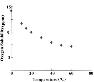
The observed corrosion behaviors of a particular metal or alloy can be superimposed on E-pH diagrams. Such a superposition is presented in Figure 2.5 for iron. The E-pH ranges of sea, natural and fresh waters derived from experimental data are also included in the same figure as a rectangular box. Many phenomena associated with corrosion damage to iron-based alloys in water at elevated temperature can also be rationalized on the basis of iron-water E-pH diagrams (Roberge 2000). Hot water heating systems like geothermal district heating systems for buildings are relevant practical examples. An excellent detailed account of corrosion damage to steel in the hot water flowing through the radiators and pipes has been published by Jones in 1993. He investigated the corrosion bevahior of iron in the pH range of 6.5 to 8 in main water, of which the E-pH diagrams are shown in Figures 2.6(a) and (b). It has been understood that minimal corrosion damage is expected if the corrosion potential remains below – 0.65V. As seen Figure 2.6, for a given corrosion potential, the hydrogen evolution is thermodynamically more favorable at low pH values. The position of the oxygen reduction lines indicates that the cathodic oxygen reduction reaction is thermodynamically very favorable. The oxygen content is an important factor in determining corrosion rates at kinetic considerations. The oxygen content of the water is usually minimal, since the solubility of oxygen in water decreases with increasing temperature as seen in Figure 2.7, and any oxygen remaining in the hot water is consumed over time by the cathodic corrosion reaction. The undesirable oxygen pickup is possible during repairs because of the additions of fresh water in order to prevent pressure loss at closed hot water pipelines and design faults that lead to continual oxygen pickup from the expansion tanks. The higher oxygen concentration shifts the corrosion potential to higher levels and Fe(OH)3 fields comes into play at these high

potential levels increasing the potential of severe or mild pitting as shown in Figure 2.5 (Roberge 2000) .

(37)

Figure 2.5. Thermodynamic boundaries of the types of corrosion observed on steel and E-pH ranges for water environments (Roberge 2000, Davis 2003)

(a) (b)

Figure 2.6. (a) E-pH diagram of iron in water at 25 0C, (b) E-pH diagram of iron in

(38)

Figure 2.7. Solubility of oxygen in water in equilibrium with air at different temperatures (Roberge 2000).

2.2. Electrochemical Reactions of Corrosion

Corrosion is either chemical or electrochemical in nature. The distinction between chemical and electrochemical corrosion is based on the corrosion causing mechanism. Chemical and electrochemical corrosion are not mutually exclusive and can occur simultaneously. Chemical corrosion is the direct result of exposure of a material to a chemical and is governed by the kinetics of chemical reactions. Chemical corrosion does not involve the generation of an electrical current. Direct chemical attack, such as the dissolutive of a material by an acid, and selective attack, such as leaching of a specific soluble compound from a material, are two common forms of chemical corrosion. Electrochemical corrosion is the dissolution of a metal through the oxidation process. Oxidation and reduction reactions occur simultaneously and are interdependent. Corrosion only occurs at the site of oxidation reactions (Degiorgi 2000).

Corrosion of metals in aqueous environment is almost always electrochemical in nature. Corrosion process requires anodes and cathodes in electrical contact and an ionic conduction path through an electrolyte, and corrosion occurs once electrons flow between the anodic and cathodic areas (Zheng 2000). The characteristics of an electrochemical reaction can be illustrated by considering the behavior of iron in hydrochloric acid. Iron reacts vigorously with HCl; hydrogen is evolved and iron gradually goes completely into solution. The reaction is:

(39)

2 2

2HCl FeCl H

F_e+ → +

This equation can be written as the following: 2

2 ₂ 2

2H Cl Fe Cl H

Fe+ + + − → + + −+

The solid iron gradually disappears and a gas is evolved. The iron converted to an iron with two positive charges. The iron is oxidized. On the other hand, the hydrogen ions have each gained an electron, thus, they have been reduced. The overall reaction can be considered as two seperate ones:

− +₊ →Fe e F_e 2 2 _(oxidation) 2 2 2H++ e− →H _(reduction)

The mechanism for the preceding case is shown schematically in Figure 2.8. The areas where oxidation occurs are defined as anode, and those where reduction takes place are defined as cathode. An electrical potential exists between the anode and cathode areas. A complete electrical circuit exists, and a current flows from anode to cathode. The faster the solid is converted to iron ions means that greater corrosion, the larger is the current flowing in this corrosion cell. Therefore, the possible anodic reactions in a system are relatively easy to predict. With cathodic reactions, there are more possibilities. The most common are:

2 2 2H+ + e→H _{...Hydrogen evolution.} O H e H

O₂+4 ++4 →2 ₂ _{...Oxygen reduction (acid solutions).}

_O ₊₂_H _O₊₄_e_→₄_OH−

2

2 ...Oxygen reduction (neutral solutions). (2.4)

+

+ ₊ _→ 2

3 _e _M

M ...Metal ion reduction.

M e

M++ → _{...Metal deposition.}

(40)

2.3. Many Forms of Corrosion

Corrosion problems can be divided into nine categories based on the appearance of the corrosion or the mechanism of attack. These are:

1-Uniform corrosion 2-Pitting corrosion 3-Crevice corrosion 4-Galvanic corrosion 5-Erosion-corrosion 6-Intergranular corrosion 7-Stress corrosion cracking 8-Dealloying

9-Biocorrosion

Many corrosion problems are due to more than one form of corrosion acting simultaneously. For instance, pitting corrosion may be caused by crevice corrosion, deposit corrosion, cavitation or fretting corrosion. Additionaly, in some metal systems where dealloying may occur, this form of corrosion may be a precursor to stress-corrosion cracking. Similarly, deep pits can act as stress raisers and serve as nucleation sited for corrosion fatigue failures.

2.3.1 Uniform Corrosion

Uniform corrosion, or general corrosion, is a corrosion process exhibiting uniform thinning that proceeds without appreciable localized attack. It is the most common form of corrosion and may appear initially as a single penetration, but with thorough examination of the cross section it becomes apparent that the base material has uniformly thinned. Uniform chemical attack occurrs in the atmosphere, solutions, and soil, frequently under normal service conditions. Excessive attack can occur when the environment has changed from that initially expected. Weathering steels, magnesium alloys, zinc alloys, and copper alloys are examples of materials that typically exhibit general corrosion. Passive materials, such as stainless steels, aluminum alloys, or nickel-chromium alloys are generally subject to localized corrosion. Under specific conditions, however, each material may vary from its normal mode of corrosion.