Indexing Multivariate Mobile Data through Spatio-Temporal Event Detection and Clustering.

UC Riverside Previously Published Works

Title

Indexing Multivariate Mobile Data through Spatio-Temporal Event Detection and

Clustering.

Permalink

https://escholarship.org/uc/item/6qr6b2ph

Journal

Sensors (Basel, Switzerland), 19(3)

ISSN

1424-8220

Authors

Rawassizadeh, Reza

Dobbins, Chelsea

Akbari, Mohammad

et al.

Publication Date

2019-01-22

DOI

10.3390/s19030448

Peer reviewed

eScholarship.org

Powered by the California Digital Library

Article

Indexing Multivariate Mobile Data through

Spatio-Temporal Event Detection and Clustering

Reza Rawassizadeh1,* , Chelsea Dobbins2 , Mohammad Akbari3 and Michael Pazzani4 1 _{Department of Computer Science, University of Rochester, Rochester, NY 14620, USA}

2 _{School of Information Technology and Electrical Engineering, University of Queensland, Brisbane 4067,} Australia; c.m.dobbins@uq.edu.au

3 _{Department of Computer Science, University College London, London WC1E 6BT, UK; m.akbari@ucl.ac.uk} 4 _{Department of Computer Science, University of California, Riverside, CA 92507, USA;}

michael.pazzani@ucr.edu

* Correspondence: rrawassizadeh@acm.org

Received: 12 December 2018; Accepted: 18 January 2019 ; Published: 22 January 2019

Abstract: Mobile and wearable devices are capable of quantifying user behaviors based on their contextual sensor data. However, few indexing and annotation mechanisms are available, due to difficulties inherent in raw multivariate data types and the relative sparsity of sensor data. These issues have slowed the development of higher level human-centric searching and querying mechanisms. Here, we propose a pipeline of three algorithms. First, we introduce a spatio-temporal event detection algorithm. Then, we introduce a clustering algorithm based on mobile contextual data. Our spatio-temporal clustering approach can be used as an annotation on raw sensor data. It improves information retrieval by reducing the search space and is based on searching only the related clusters. To further improve behavior quantification, the third algorithm identifies contrasting

eventswithina cluster content. Two large real-world smartphone datasets have been used to evaluate

our algorithms and demonstrate the utility and resource efficiency of our approach tosearch.

Keywords:spatio-temporal; clustering; event detection; mobile sensing: contrast behavior mining; human behavior

1. Introduction

The proliferation of mobile and wearable devices offers researchers opportunities to detect, identify, and classify human behavior. New computational paradigms, in combination with wearable sensors have powered the “quantified self” and “mobile health” movements, in addition to the renewal of interest in underutilized paradigms, such as “lifelogging” and “personal informatics” among other terms for self-tracking to improve personal performance. All of these systems benefit from sensor data that have been collected by mobile and wearable devices from the user’s environment and behavior.

These data aremultivariate(e.g., accelerometer and GPS), typicallysparseandtime-stamped[1].

However, despite the richness of this data, there remains a lack of appropriate searching and information retrieval mechanisms that are able to filter sensor data within the resource limitations of small mobile devices. Therefore, data analysis should be done on a remote host, such as on the cloud

or cloudlet [2]. However, this will raise network response time and privacy related issues [3].

We believe virtual assistance devices or applications with conversational agents could work in synergy with human memory, enabling users to recall previous life events through lifelogging.

For example, a user can ask her virtual assistant“How many times did I visit the gym last month?”or

“How long did I spend in traffic during my daily commute?”. In spite of the obvious utility of such a

system, such search and querying mechanisms for mobile health applications (e.g., Google Fit [4],

Samsung Health [5] and FitBit [6]) on personal assistants (e.g., SiRi [7] and Cortona [8]) do not yet

exist. Existing mobile health applications continuously collect data, but they only provide temporal browsing and graph based visualizations. Graph illiteracy is a major challenge among individuals,

even in developed countries [9], that has affected the usability of mobile health applications [10].

Any requirement for manual intervention in these systems is a barrier to adoption [11]. Therefore,

frequently annotating the data manually is not useful. However, manual annotation is inevitable and we cannot completely remove it. On the other hand, little work has addressed index creation frommultivariate temporal sensor data. An annotation/indexing mechanism can facilitate higher-level searching and querying of datasets composed of temporal sensor data.

In response to these challenges, this paper is aimed atspatio-temporal indexingof multivariate

temporal data to reduce the search space for facilitating human-centric searching of queries.

Our approach is toward enabling mobile devices to search their collected data in a reasonable time with less resource utilization. In particular, our contribution is a pipeline of three algorithms that improves search execution time and resource-efficiency, as follows:

• We describe aspatial event detectionalgorithm to detect daily life events from raw data (mobile

sensor data). Daily life events are typically grounded in specific times and locations, and this spatio-temporality can be extracted from sensor data. Converting daily activities into discrete spatial events is our first step toward annotating and indexing the raw data. Since location data from mobile devices are sparse and not always available, our algorithm should be able to cope

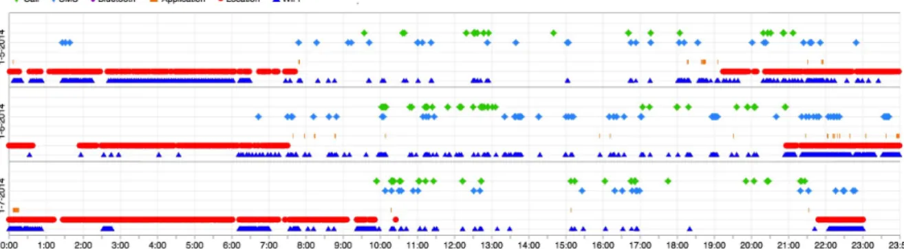
with uncertainty and sparsity. For instance, Figure1shows a visualization of three days of data

from a user. It shows that location data (•) and WiFi data (N), which could be used for location

estimation, are not always available.

• Given that human mobility behavior is known to be predictable, at least in the aggregate [12],

our second contribution is an unsupervised spatio-temporal clustering mechanism that

identifies similar daily life-events and annotates them based on their correlation withlocation

changesandtimes. In other words, life events during a routine behavior, e.g., commuting to a work at a specific time of the day, or going to the movies on weekends, will tend to map to the same cluster.

This spatio-temporal clustering provides a higher level of annotation (index), and in turn reduces the search space.

• Our third contribution is exploiting the content of each individual cluster to allow us to identify

contrasting events inside a cluster. The identification of contrasting events (behaviors) is a

major step toward the enrichment of sensor datainsidea cluster, and thus refining the described

spatio-temporal indexes. For example, consider a user who visits a coffee shop for two purposes, either to chat with friends or to work. Since both chatting and working take place in the same location, and, at the same time, spatio-temporal event detection alone may not suffice to distinguish between these two distinct user behaviors. However, data from the mobile or wearable device microphone can differentiate between working and chatting (at the same location/time).

Therefore, a contrast-set detection [13] method is better positioned to delve deeper into the content

of our spatio-temporal clusters. Furthermore, first searching clusters with fewer contrasting events could improve search execution time as well.

Figure 1.UbiqLog life log visualization of three days of data for a single user (best viewed in color).

To concretely ground these concepts, consider two application scenarios that would benefit from using our algorithms:

(i) User 1 goes to the gym on a regular basis, and maintains her diet. Nevertheless, she starts

gaining weight. Using the contrast event detection algorithm, she realizes that she recently began spending less time on cardio training in favor of weight training, which is a prime suspect for her weight gain.

(ii) User 2 has a flexible working schedule. Through the spatio-temporal event detection algorithm, he can estimate how much time he spends commuting to work on average, and then find out the best time/day to commute.

These two examples exhibit the utility of using the spatio-temporal annotation (indexing) within

higher-level applications. In other words, our algorithms facilitates searching throughreducing the

search spacebased onclusteringand analyzing clusters based on theircontrasting events. Furthermore, prioritizing the search based on clusters with a lower number of contrasting events could slightly improve the search execution time. There are promising approaches for analyzing mobile data to

extract behavioral patterns [1,14,15]. However, based on our knowledge, this is the first work that

relies on thespatio-temporalityof the mobile data for annotating other sensor data, clustering them and

ordering the clusters based on their contrasting events. In other words, this is the first work to employ

such a facility toward enabling on-device [3] search operations for end users.

Note that, except event detection, which does not have any new parameters, each of our algorithms has only one parameter to configure (in total two parameters, one for spatial clustering and one for contrast behavior detection) and, in the evaluation section, we report parameter sensitivity analysis in detail. Parameters for the event detection are either constant or they have been chosen based on optimal values from previous works. Each algorithm could be used separately as well. For instance, a user can choose another event detection method, not using contrast behavior detection and only use the temporal clustering algorithm.

Implementing the end-user application which hosts this search facility is not in the scope of this paper. The end-user query parsing is the task of the application that hosts our methods. Moreover, our algorithms are not able to completely remove the burden of manual location annotation, despite mitigating it significantly. They can be used inside applications (as middleware) that require searching mobile data or converting raw data to higher-level spatio-temporal information, and reducing the need for manual annotation.

2. Problem Statements

Daily events in a person’s life (e.g., going to the gym) can be recognized by mobile and wearable

devices. Here our focus is onspatio-temporaldaily life events, or in other words activities of daily life.

As such, this work does not directly support higher-level and longer term life events, such as getting married or attending graduate school. Moreover, life events contain nested events, which are not

covered in this work, e.g., being at work may be associated with nested events such as drinking coffee,

moving to different offices, etc. Our work can distinguishdiscretedaily life activities, based onlocation

changes, such as driving to work or going to a restaurant.

Notwithstanding these limitations, we believe this work is among the first toward quantifying spatio-temporal dynamics from sparse multivariate temporal data from smartphones.

2.1. Spatial Event Detection

Daily lifeeventsoccur in a specific locationata specific time, and can be understood as a set of

actionsfrom the device a user is carrying. Each action,a, can be modeled within a 4-tuple arrangement:

a=<S,D,T,L>.Sdenotes the context sensor name (or attribute name),Dis sensor data (or value of

the attribute),Tis the timestamp of the action, andLis location of the action. Geographical coordinates

in most real-world cases does not exist. Therefore, we focus only on location state and accurate

geographical coordinates, i.e.,L. Each user life event can be formalized within a specific timeT

and specific locationL. Previous works [14,16] have proposed using spatial changes as a primitive.

However, a single location can be associated with disparate actions, i.e., home, work, etc. Thus, we need to consider the finer granularity of actions used to model an event. In other words, an event

eis composed of a finite set of actions: e = {a1,a2,a3, . . . ,an}and all these actions have the same

location state (specific constant location). If the location has changed, it is the end of the current

event and the beginning of a new event. Lis the constant in the following definition of an event:

e = {< S1,D1,T1,L >,< S2,D2,T2,L >, . . . ,< Sn,Dn,Tn,L >}. Therefore, the event e can be

described as:

e={ai : l(ai)∈(Θ∨∅),∪l(ai) =l,Tmin≤t(ai)≤Tmax}, (1)

wherel(a)is the location, andt(a)is the time of the actiona, while each event is bounded by specific

temporal borders. By constant location, we do not mean the exact latitude and longitude of a location (For the sake of simplicity, we refer to the movement state, location changes, as ’location state’);

we mean a movement state i.e.,moving,stationaryandunknown. Unknown is used when a location

is not available, e.g., in Figure1between∼1:30 p.m. to∼3:00 p.m. on 1 July 2014, because there is

no WiFi and geographical coordination data available. Here, the process of location annotation is manually assigning labels to the identified location state, based on time of the day, which is used in

our evaluation section. The first question is to identifyl(a), which represents the location. Since it

is constant in each event, we useΘto denote the location, either “moving” or “stationary”. Due to

pervasive device restrictions, e.g., GPS does not work indoors, the user turns it off, etc., it is not possible

to continuously get location, thusl(a)is either null orΘ. In addition, the union of all locations of

actions inside an event are a single location state. At this point,Θis a geographical coordinates object

(if it exists). Later, it will be a location state, which we will describe it in this section.

2.2. Temporal Clustering

To index events, the second challenge is to identify and cluster similar events that occur (i) at about the same time interval in consecutive days and (ii) in the same location state (moving, stationary or unknown). For instance, events that include “daily commute to work” will be assigned to one cluster, and events that include “attending the gym in the evening” will be assigned to another cluster. Note that this clustering will be done for each user separately and no information will be shared between users.

Routine human behaviors do not usually occur at a fine temporal granularity [1], and there is a

temporal uncertainty. For instance, a person may go for a coffee break one day at 4:34 p.m., the next day at 4:31 p.m. and the day after that at 4:20 p.m.. Given this, any model of human behavior should be flexible enough to be invariant to such minor timing differences.

To handle this need for flexibility in our model, we define atemporal interval,λ. This interval will

be used for comparison between the start of events (lower bound) and also the end of events (upper

bounds). Later, in Section4, we will describe more about the use ofλ. With this notation, we formally

define the task of temporal clustering of events as the following:

Definition 1. Given a set of events C and a temporal intervalλ, the objective is to categorize events into

k different sub-groups, i.e., clusters,{Ci}ki=1. For each pair of events ex, eyin any cluster Cithe following constraint holds, where ex(a)presents an action a inside event ex.

∀(ex,ey)∈Ci: (

|min(t(ex(a))−min(t(ey(a))| ≤λ,

max(t(ex(a))−max(t(ey(a))≤λ,

(2)

In other words, for each pair of eventsexandey, the temporal difference between their lower

and upper bounds should not exceed theλtemporal interval. However, there are events that could

be routine, but they occur at very different times of the day. Those events cannot be handled by our approach.

2.3. Contrasting Events Identification

One can argue that simply clustering based on spatio-temporal properties of activities is too much of a generalization for human behavior. For instance, a user could go to the gym some times for cardio training and sometimes for weight lifting. In these instances, the spatio-temporality of both events are similar, i.e., they stay in the same cluster. However, they are different behaviors. This example shows that we need to have a deeper overview of behaviors.

After temporal clustering, we go one step further and compare/contrast the contents of each individual cluster. This is an important step toward augmenting cluster content. Consider the previous example in which a person regularly visits the same place each weekend. Sometimes, she performs

weight lifting and sometimes she performs cardio training. Figure2is a toy example that visualizes

a daily routine behaviors of a user. In this scenario, the spatial and temporal similarity failed to distinguish the contents of her activities inside the gym, and thus we need to examine more closely the activities that are happening “inside” the cluster.

D a y 1 D a y 2

Figure 2.A presentation of constrasting activities bewteen two evetns of the gym cluster (the cluster is marked with red dotted area), i.e., cardio training and weight lifting.

Traditionally, contrast-set mining is used to identify meaningful differences between groups by

finding predictors that discriminate between the groups [13]. Inspired by this concept, we define that

two eventsemandeninside a cluster are contrasting/dissimilar if they fail to share at leastωnumber of

common actions, whereωdenotes thedissimilarity thresholdcontrolling the flexibility of the algorithm.

For example, in Figure2, ifω=1 the events in the gym cluster are all considered similar. However,

ifω=2, then the two gym events in that cluster are considered to be dissimilar.

Contrasting events can be identified by the followingΓcfunction:

Γc(em,en) =    1, i f ∑ii≤,j=m1,j≤nem(ai)∩en(aj)≥ω, 0, otherwise, (3)

wheree(a)function denotes allactionsinside the evente. If the comparison between two events returns

fewer thanωactions, then theΓcoutput is false (0), otherwise this function returns true (1). False output

means these events are not significantly different (i.e., not contrasting behaviors). Our experiments mostly show that events inside a cluster have a similar number of actions; therefore, there is no need to use a Jaccard similarity, just relying on the intersection is enough. Going back to the example of User1,

ifωnumber ofactions(e.g., physical activities that can be measured via an accelerometer) that she

performs in her two gym sessions are different, then the two gym events are considered contrasting events, e.g., cardio versus free weights. Therefore, the problem of contrast event detection can be formalized as:

Problem 1. Given a cluster of events Ciand a dissimilarity thresholdω, the objective is to identify contrasting

events inside the Cicluster by detecting any pair of events emand en, which holdsΓc(em,en) =1.

This problem formulation exploits the intrinsic multivariety of the data. In particular,

our experimental datasets contain data objects from different resources (multivariate), but this model links them together via timestamps and converts different timestamped data as fine-grained units.

3. Datasets

Two smartphone datasets have been used for our experiments, UbiqLog [17] and Device

Analyzer [18]. We chose these two datasets because in the real-world there are many different makes

and models of smartphones, and each device has its own restrictions and specifications for hardware and software. This affects the quantity and quality of the data. As we are demonstrating our algorithms in a real-world setting, we have chosen these two datasets because both have collected data outside a lab setting in the real world.

UbiqLog[19]: An open source Android-based life logging tool [20] has been used to create the UbiqLog dataset. It includes 9.78 million records of users’ detected WiFi, Bluetooth, application usage, SMS, call, physical activity (based on Google Play Services) and geographical location. The capacity for location extraction varies based on availability and device status, e.g., GPS, Cell-ID and Google

Play Services Location API. Figure1shows a visualization of three days of a single user’s data in

the UbiqLog dataset. Thex-axis represents the time of the data, and each sensor has a different

color. Table1provides details about the UbiqLog dataset records, whilst another report [11] describes

more about the data collection experiment. All records are semantically rich and are human readable. Therefore, there is no raw sensor data, such as accelerometer data, in this dataset.

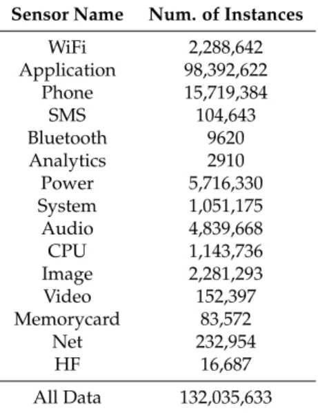
Device Analyzer[21]: This is the largest smartphone data-set created and is based on hardware status and device configuration of Android smartphones in which users have installed the Device Analyzer app. It contains raw sensor data for more than 30,000 users. However, our interest is only in the data that is common with the UbiqLog data. This is because UbiqLog is focused on human-centric data that can be collected via smartphones. Device Analyzer is a more hardware-oriented approach

and includes detailed information about device status changes. Table2shows the number of records

for the 35 random Device Analyzer users.

Although the real focus of our algorithms is on user-centric data, to demonstrate the versatility of our approach, we have performed our evaluations on both datasets. We have randomly selected 35 users from Device Analyzer and 35 users from UbiqLog, which means in total we have experimented on 70 users.

Table 1.Number and types of sensors in the UbiqLog dataset. Sensor Name Num. of Instances

WiFi 8,750,111 Location 725,560 SMS 28,849 Call 99,022 App. Usage 45,803 Bluetooth 117,236 Activity State 15,641 All Data 9,782,222

Table 2.Numbers and types of sensors for 35 random users’ data from Device Analyzer dataset. Sensor Name Num. of Instances

WiFi 2,288,642 Application 98,392,622 Phone 15,719,384 SMS 104,643 Bluetooth 9620 Analytics 2910 Power 5,716,330 System 1,051,175 Audio 4,839,668 CPU 1,143,736 Image 2,281,293 Video 152,397 Memorycard 83,572 Net 232,954 HF 16,687 All Data 132,035,633 4. Algorithms

The first step of our approach is to extract events based on the spatio-temporal properties of sensor data, for each user. To identify events from raw data, we introduce a spatial change point detection method. Then, based on both temporal borders and spatial state, we introduce temporal interval based clustering to group similar events together. As it has been described, spatio-temporal quantification alone may not suffice for all application scenarios. Therefore, elements of each cluster are further

analyzed to identify dissimilar events. Since privacy issues currently appear insurmountable [22,23],

all proposed algorithms are completed separately for each user, and information is not shared among users.

4.1. Spatial Change Point Detection

Event identification is based on location state changes. As described, location refers tomoving,

stationary or unknown. This notion of location is more limited than in other research efforts, which consider geographical locations. However, in the real world, we do not have access to the geographical coordinates 24/7. Therefore, this definition has the advantage of greater availability,

which is required in a real-world application. Furthermore, Figure1shows a small time shift in routine

human behavior. The displayed dots are not just GPS data but a combination of Cell-ID, GPS and

Google API. While a few research efforts [24,25] focus on extracting locations from acombinationof

different location data sources (fusion), several efforts focus on collecting and mining location traces

from asinglesource of information [26,27] and have demonstrated promising results.

Note that our approach is focused on the data that is being collected from the users’ device

be obtained from sources including Cell-ID, WiFi, wireless beacons, etc. Cell-ID is too imprecise to be used for location estimation, and, due to limited battery power, users often do not enable GPS. Therefore, a more reliable source, such as a combination of both WiFi and Cell-ID (which are more resource efficient in comparison to GPS alone), should be used for estimating location. In other words, a location estimation algorithm is assumed to extract location from a combination of sensors.

Our change point detection (location estimation) algorithm receives a set ofactionsandsignal type

as inputs and it returns a list ofevents. Actions are a 3-tuple of attribute (sensor name), value (sensor

data) and timestamp. Signal type can be WiFi only (e.g., Device Analyzer data) or a combination of sensors. An event includes a location state, start time, end time, and a finite set of actions. The following shows a simplified example of raw sensor data in a time slot, i.e., between 12:00 p.m. to 12:30 p.m. Since the WiFi is not repeated, we consider this time slot as “moving”.

{{name:"call",val:"1800xxx", time:"12:02-12:03"}}, {name:"WiFi",val:"BSSDID_1", time:"12:04"},

{name:"activity",val:"walk-910s.", time:"12:04-12:18"}, {name:"WiFi",val:"BSSDID_x", time:"12:26"}.

The following shows an example of an event with four actions, after change points have been identified and annotated, i.e., “location state”.

{location_state:"moving",time:"12:00-12:30", actions:{{name:"call",val:"1800xxx", time:"12:02-12:03"}, {name:"WiFi",val:"BSSDID_1", time:"12:04"}, {name:"activity",val:"walk-910sec.", time:"12:04-12:18"}, {name:"WiFi",val:"BSSDID_x", time:"12:26"} } }.

Note that the algorithm checks the signal type, either Wi-Fi or combination of all location signals. If both Wi-Fi and geographical location exist, the algorithm prioritizes the geographical location over Wi-Fi (due to its superior accuracy).

If it is only Wi-Fi, it searches for consecutive timestamped WiFi logs. If such a sequence exists,

and all its elements (i.e., BSSID of WiFi) are unique, this is a sign of amovingevent. For example,

a sequence of not repeated WiFi BSSID asWx,Wy,Wzis a sign of a moving event. Therefore, a moving

event (with its start time and end time) will be created and appended to theeventslist. Otherwise, if it

is not a moving event and there is a sequence of elements, but they are not unique (i.e., repeated BSSID),

the algorithm identifies them as astationaryevent. For instance, a 60 min sequence of repeated WiFi

BSSID asWx,Wy,Wa,Wx,Wb,Wypresents a stationary event. If in a time interval of 60 min no WiFi

signal exists at all, and all other location signals are not available either, the algorithm creates an

unknownevent. The algorithm uses a time interval of 60 min because it has been identified [1] that the temporal granularity of 60 min has the highest accuracy for routine behavior identification. In other words, this time interval could be assumed as a smoothing factor.

All events include a start time and end time. In short, when the algorithm finds a number of WiFi

BSSIDs (let us say names for simplicity) repeated together, it creates astationaryevent. However, if the

WiFi names changes and they are not repeated, it creates amovingevent. If none of the described cases

exist, the algorithm creates anunknownevent.

If the signal type is not just WiFi and it is a combination of GPS, Cell-ID and a 3rd party location service such as the Google Play service, the algorithm takes a different approach. If geographical coordinates exist (GPS or a similar 3rd party service), the location status is easily computed. To calculate this type of location state, it computes the difference between two consecutive geographical coordinates.

If two signals have a distance more than thedistance thresholdδdand are equal to or more than the temporal thresholdδt, then the algorithm marks the target time frame (event) asmoving. Otherwise, if the

distance is less thanδdand more thanδt, it marks them asstationary. If no location signal appears after

δttime, then the algorithm creates a new event and marks the event asunknown. This event continues

until a new location change appears. When a new location signal appears (that creates a different location state), it ends the previous event. Ending an event means the algorithm closes the event with the timestamp of the last element in the dataset. Then, a new event is created with the timestamp of the new location element that has been most recently read.

Note thatδd is a fixed number and varies between 800 to 1000 m in cell tower installations;

e.g., in the city of the UbiqLog experiment, it is fixed to 800 m.

The UbiqLog dataset shows that most of the time GPS is turned off (based on its real-world nature), there are very few GPS logs and they occur mostly when users are navigating. Most location logs are from Cell-ID; and thus it is not possible to precisely estimate location (because of relying on

Cell-ID instead of precise coordinate) [25]. In particular, when the location change is noted, there is an

ambiguity as to whether the location has truly changed or just the cell tower has changed (i.e., handoff). Nevertheless, there is a fixed precision associated with the location extracted from the Cell-ID. Let us

assume the precision distance isδd, (in the city of the UbiqLog experiment, the precision distance

between Cell towers was 800 m) and a temporal precisionδt. To understand this problem, consider the

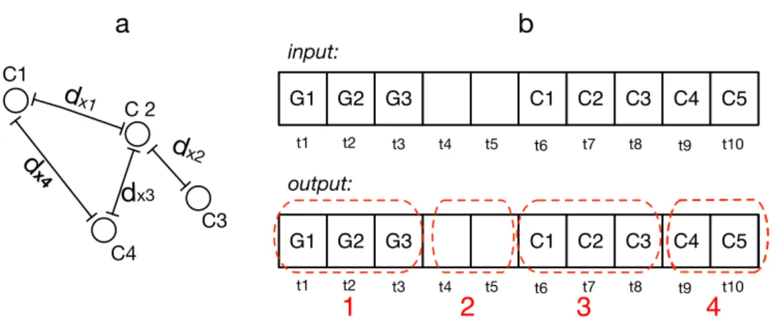
example in Figure3a. There we haveC1,C2,C3,C4. Ifdx1+dx2 > δd, this means that the user is

moving. Ifdx1+dx3>δdbut the distance betweenC1andC4:dx4<δd, then the user is inferred to

be stationary and not moving. Therefore, when the algorithm calculates only the distance between two consecutive points, it might face a problem. To resolve this issue, when the location is based on

Cell-ID, the algorithm calculates the location distance betweenthreeconsecutive points rather thantwo.

Figure3b shows a trace, which has a combination of GPS(G) and Cell-ID(C) locations. It shows that

four Cell-IDs have been recognized and C4 has not been categorized as the same event. Based on cell

tower distribution [26],δdmust be 800 to 1000 m (cell tower distances) to check whether or not there is

a location change or not, and five minutes has been assigned toδt.

C1 C 2 C3 C4

d

d

d

d

1

2

3

4

a

b

Figure 3.(a) Four consecutive locations from Cell-ID; (b) four events have been detected, the first three elements contain GPS, and then with two elements marked as unknown. Three later elements, C1, C2, C3 contain cell IDs and show another movement until the point C4. The geographical distance between C4 and both C3 and C2 is less thanδd.

Setting δt to five minutes is extracted from the evaluation conducted in the data collection

experiment [11]. Therefore, in this paper, we do not evaluate the parameter sensitivity ofδt,δdand the

time intervals.

The computational complexity of the this spatial change point detection algorithm is linear because, even if we assume all locations are Cell-ID, there is a need for a comparison of each element

4.2. Temporal Clustering

The second step is to cluster similar user events of a person based on theirspatialandtemporal

similarity. Events inside a cluster have the (i) same start time, (ii) same end time and (iii) same location state, which was identified in the previous stage.

We interpret similar spatio-temporal events as an indicator for a routine behavior, e.g., commuting to work, going to the park on weekends, etc. Similar events are collected in clusters. As it has been

described in Section2, we need to handle the slope of human timing of similar events and thus useλ.

λcan be interpreted as a reasonable “slope interval” to calculate similarities between events. Figure4

shows aλinterval that covers the start times (lower bound) of two (visually) similar eventsS1-3and

S2-3from two consecutive days. Clusters are not overlapped.

S1-3 S1-2 S2-3 tn Day 1 t0 S1-1 ti ti+2 S2-4 S2-2 S 2-1 S4-3 S4-2 S4-1 S4-4 S3-1 S1-4

Day 2 Day 3 Day 4

Not Covered by λ

Time of day

λ

Figure 4.An example of four days with spatio-temporal change points, Day 3 is on a weekend. The fix λdisables the algorithm from recognizing Day 4 events properly in their cluster. In particular,S1-3, S2-3andS4-3should belong to the same cluster. However, by not movingλ,S4-3can not fit into the cluster ofS1-3andS2-3.

Algorithm1describes our temporal clustering approach.λand a list of events,inEvents, which are

ordered based on timestamps, are inputs. The algorithm iterates through all events; then, it selects

the first two days through theinitiatemethod, line 3.ebaseis the event list of the first day andesecond

is the event list of the next day. On line 5,similarSTmethod compares the spatial and temporal data

of two events from each day. If they are similar, and a cluster with their spatio-temporal properties

exists (checked byexistsSim) then the algorithm adds both events into their respective cluster, on line 7.

Otherwise, if they have similar spatio-temporal properties but no cluster exists with the similar spatio-temporal properties, the algorithm creates a new cluster on line 9 and adds both events into this

new cluster. If none of the above conditions are met, both events will be added totmpNSlist (list of

orphan events), line 11.

Days are compared sequentially, but there are events that do not occur every day but occur frequently, such as going to the gym twice a week or events originating from weekend activities,

e.g., going to the movies. To cluster these events, dissimilar events will go into thetmpNSlist (line 11).

After the first loop, which compares all events and assigns them to their cluster, the algorithm orders

the content oftmpNSbased on time, on line 14. Then, it starts iterating through them on line 15. If two

consecutive events insidetmpNSare similar, and their spatio-temporal properties are similar to one of

the exiting clusters (existSimmethod on line 15 checks this condition), then these two events will be

added to that existing cluster, on line 18. Moreover, these events will be removed fromtmpNSbecause

now they have a cluster. If they are not passed to any cluster but their spatio-temporal properties are similar, a new cluster to host them will be created on line 20 and collect them. Nevertheless, if none of these conditions apply, these events do not have any similar events and they will be added to a list of

Algorithm 1: Temporal clustering of events. Data:inEvents,λ

Result:ClustList,nonsimilar 1 while(!inEvents.isNull)do

2 // create 2 event lists (base,second) from current 2 days.

3 e_base[_],e_second[_]←initiate(inEvents.currentDay,inEvents.nextDay);ct←0; //ct is a counter

4 forall events in e_basedo

5 if(similarST(e_base[ct],enext[ct],λ) =t)

6 AND (existsSim(e_base[ct],ClustList) =t))then 7 ClustList.update(e_base[ct],enext[ct]);

8 else if(similarST(e_base[ct],enext[ct],λ) =t)then 9 ClustList.addNew(e_base[ct],e_next[ct]); 10 else 11 tmpNS.add(e_base[ct]); 12 ct+ +; 13 ct←0 ; 14 tmpNS.order(); 15 forall events in tmpNSdo 16 if((similarST(tmpNS[ct],tmpNS[ct+1],λ) =t) 17 AND (existsSim(tmpNS[ct],ClustList) =t))then

18 ClustList.update(tmpNS[ct],tmpNS[ct+1]);tmpNS.remove(tmpNS[ct],tmpNS[ct+1]); 19 else if((similar(tmpNS[ct],tmpNS[ct+1],λ) =t)then

20 ClustList.addNew(tmpNS[ct],tmpNS[ct+1]); tmpNS.remove(tmpNS[ct],tmpNS[ct+1]); 21 else 22 nonsimilar.add(tmpNS); 23 ct+ +; 24 return(ClustList);

Human behavior slowly evolves over time [1], which means, among other phenomena,

similar events and their timings will change over time. To resolve this issue,λwill be moved between

days, but it is a fixed variable. In particular, the algorithm will not use one day as a benchmark and

then compare the other days to that single day. Figure4neglects the spatial property of an event for

the sake of readability, and visualizes the problem of not movingλ. The example shows four days

within their temporal events identified.S1-3andS2-3could stay in the same cluster, butS4-3is not

covered by theλthreshold, despite the fact that we can see it belongs to the same cluster. In addition,

S1-2andS2-2have a similar end time, but if we do not moveλ,S4-2also lacks a similar end time.

Because of a minor time variety of daily routine behaviors, theλis changing. If two events are

similar, which means their upper bound and lower bound are≤ λ, thenλwill be updated as the

averageof upper bound or lower bound between two similar events. Otherwise,λwill be not changed.

Each day will be compared with another day, which requiresnnumber of comparisons. In the

worst case, the content of orphan event list (nsimilar) is equal ton−1 and again we have about

2(n−1)number of comparisons. This means that the complexity of this algorithm isO(2(n−1)),

which is linear.

4.3. Detecting Contrasting Events

An individual’s frequent presence in the same location state at the same time does not mean she necessarily engages in exactly the same behavior. In addition, an event may be too prolonged to quantify its content. For instance, a user could stay at home for a day but have significantly different

activities, such as recuperating from an illness or working from home. To identify such differences,

we propose a novel contrast behavior (CB) detection approach for eventsinside a cluster. Our CB

detection algorithm is inspired by contrast-set mining algorithms [13]. Some research considers

contrast-set mining as a rule discovery [29], but we have a different interpretation, tailored for mobile

data that are multivariate temporal data.

Algorithm2presents a method to compare the actions of each eventinsidea cluster. The algorithm

receives a cluster,inC, andω. As previously described,ωis the threshold for uncommon actions in

each event. The algorithm identifies the contrasting events in each cluster and at the end reports for each cluster how many of its members (events) are contrasting and how many of them are similar. The result of this algorithm is useful for searching because it enables the search algorithms to prioritize the clusters, based on the number of similar events.

Algorithm 2:Contrast behavior identification from events inside a cluster. Data:inC,ω

Result:eventList

1 ct←0; //ct & 2ct are counters 2 forall(events in inC)do

3 //get an event and compare it with others 4 eventM←inC.event[ct]; 2ct←0 ; 5 forall (events in inC)do

6 if(eventM.actions!=inC.event[2ct])then

7 if(di f f(eventM.actions,inC.event[2ct])>ω)then 8 result.add(eventM.actions,inC.event[2ct]); 9 2ct+ +;

10 ct+ +; 11 return(Result);

On line 2, the algorithm iterates through the number of events in a cluster (line 5) and compares

each event (eventM) actions with other events inside that cluster, on line 6. Thedi f f method (line 7),

compares two events and, if the number of different actions is larger than theωthreshold, then those

events are counted as contrasting behaviors. This comparison is measuring theexact similarity

between each action. We did not use other similarity metrics such as Jaccard coefficient because our empirical experiments show that the number of actions of events inside the cluster are either equal

or the difference is very insignificant. At the end, they are collected in theResultset and returned.

This comparison is measuring theexactsimilarity between each action.

A large number of dissimilar events indicates that the user’s activities are not routine. Theω

value is application dependent. It also depends on the temporal event size, the purpose to which outputs are used, and how that benefits from our approach. For instance, if an event size is about a day (e.g., a device is stationary during the day) contrasting behaviors do not reveal much about the

underlying semantics of the data. Assumingnnumber of events are inside a cluster, each event inside

a cluster is compared with other events in the cluster. Therefore, the algorithm hasn2comparisons and

its complexity will beO(n2). However, the number of comparisons is limited to only the number of

events inside a cluster. Therefore, the number of comparisons is small (e.g., two to eight in a UbiqLog

dataset) and thus the performance overhead is insignificant. Section5.3reports this cost in detail.

Note that the contrast behavior detection provides a minor semantic improvement, i.e., annotation, on the actions inside a cluster and still more knowledge extraction is required on the data. In particular, contrast behaviors will be used mainly to order clusters for the search. The implementation of the annotation, such as geo-fencing, drives the conversion of sensor data to a higher level of information in the task of the application that uses our algorithms. Therefore, there is still a need for manual annotation, but our approach significantly reduces it. For instance, for the ground truth dataset,

we have implemented a simple annotation, based on users’ manual labels, e.g., home, gym, work, etc. Users annotate one event only once in a cluster, and then it will be distributed among other events in that cluster.

5. Experimental Evaluation

This section demonstrates the utility and efficiency of the proposed algorithms in detail. In addition, we report about the spatio-temporal clustering impact on search execution time reduction and battery utilization, which is our main objective. Firstly, we begin by evaluating the event detection. Then, we demonstrate our experiment for cluster detection, its impact on search time and energy use. Afterwards, we demonstrate the contrast behavior detection accuracy and its impact on searching.

5.1. Event Detection

To evaluate the efficiency of the event detection algorithm, first we have built a ground truth dataset. This dataset will help us to analyze the accuracy of detected events and finding the optimal

value forλ.

5.1.1. Ground Truth Dataset

We have created a ground truth dataset that includes manual labels. In particular, 10 participants have used UbiqLog, and 10 other participants have used a Device Analyzer for two weeks. Participants included 7 females and 13 males, (mean age = 27.3, SD = 4.5). Participants have manually labeled their location state changes. They label only one event in each cluster, i.e., first event, and the rest of the labels will be distributed automatically to the other events in each cluster.

Participants can choose between one of these predefined labels [30]: “Commute”, “Sport”, “Home”,

“Work”, “Leisure” and “Other”. They have installed a simple tool that enables them to choose their location state changes manually from the given list.

The resulting dataset, with λ=30’, contains 34 distinct clusters (not shared between users).

Our algorithms have extracted 237 events, 69 of them were contrasting events, ω = 2. Later in

the evaluation section, we describe the policy of choosingω=2.

5.1.2. Accuracy of Detected Events

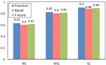
The first question for the event detection evaluation is whether the identified location state of the event is correct. Based on real-world settings, the location state could be detected from three different states: (i) there are no geographical coordinates, and only WiFi data can be used, i.e., WiFi Location (WL); (ii) WiFi combined with geographical coordinates, i.e., WiFi/Geographical Location (WGL); (iii) the GPS sensors on the phone are always on, and location is stored using only geographical coordinates, i.e., Geographic Location (GL). It is unrealistic to assume uninterrupted 24/7 sensing of geographical coordinates. Nevertheless, participants were asked to implement all three statuses during the experiment and never turn off their phone or use airplane mode. Their labels have been used to calculate “precision”, “recall” and “F-score” for the evaluation. In particular, “true positives” are location states that are similar both in user labels and the system, and they are not “unknown”. “False positives” are location states that are identified by the system and not “unknown”, but users have labeled them differently. “False negatives” are location states that have been identified by the system as “unknown” and the users have labeled them either as “moving” or “steady”. Clearly,

they did not use the “unknown” as a label. Figure5reports about the accuracy of these three described

states. The low number of false positives leads precision to be higher than recall in WGL and GL. Due to several false negatives, WL has a lower recall than other methods, which is due to the WiFi sensor that is mostly turned off to preserve the smartphone battery. In other words, in the absence of WiFi and GPS, the system marks these data as “unknown”, but clearly participants have provided labels.

0.63 0.82 0.9 0.6 0.8 0.88 0.61 0.81 0.89 0 0.2 0.4 0.6 0.8 1 WL WGL GL Precision Recall F-Score

Figure 5.Accuracy of the three different location state estimation approaches based on available data type(s); Wifi Location (WL), Wifi/Geographic Location (WGL) and Geographic Location (GL).

Furthermore, Table3reports the accuracy of location states based on the type of location state

(stationary vs. moving). In other words, Figure5presents the accuracy of different sensor settings,

whilst Table3presents how accurate each sensor setting can measure the location state (moving vs.

stationary). It shows that using GPS significantly increases the accuracy of detecting moving events. As expected, WiFi alone (WL) has the lowest accuracy because of the lack of geographical coordinates. Note that, since the number of movement and steady (stationary) events are not always equal, we can

not average results of Table3to get the result of Figure5. Therefore, we have asked participants to

label each event individually.

Table 3.Average accuracy of different sensor settings for each location state.

WL GL WGL

Moving Steady Moving Steady Moving Steady F-score 0.26 0.91 0.90 0.78 0.90 0.92 Precision 0.48 0.88 0.85 0.74 0.93 0.94 Recall 0.11 0.93 0.96 0.79 0.92 0.92 5.2. Clustering

To evaluate the utility of the proposed clustering algorithm, first we compare scalability with other clustering methods along with a comparison of quality. To compare our algorithm with representative algorithms, we have converted the combination of sensor name and its value to the number, and we

have normalized time of day with five minutes precision (temporal granularity [1]) and converted it to

a number.

Through parameter sensitivity analysis, we get the most accurate results with the following parameters for clustering algorithms: K = 9 for k-mean, minPts = 3, eps = 5 for DBSCAN and k = 8 for the hierarchical clustering.

Moreover, to demonstrate the capability of the clustering algorithm to handle non-daily routines, we analyze the accuracy of our clustering algorithm in two different modes (neglecting orphan events

versus using them). Then, we report about the parameter sensitivity ofλ. Afterwards, we demonstrate

5.2.1. Scalability of Clustering Algorithm

The execution time and maximum memory usage are indicators of the scalability of an algorithm. Here, we compare our clustering execution time and memory usage to well-known clustering algorithms, i.e., K-means, Hierarchical clustering (HCA) and DBSCAN. We have chosen these algorithms because most existing works on mining mobile data were focused on using one of these representative algorithms.

Note that there is no state-of-the-art spatio-temporal clustering developed for smartphone data, i.e., to extract location from WiFi and geographical coordinates. Therefore, we have chosen to compare our clustering approach with well-known methods.

Since the algorithm should run on small devices, this experiment ran on a smartphone using

an SPMF library [31] to implement the clustering algorithm. The test device was a Moto G 2nd Gen.

(Motorola, Chicago, IL, USA) with a quad-core 1.2 GHz CPU and 1 GB RAM. Our clustering algorithm

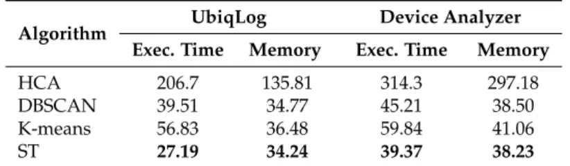
is abbreviated as ST ( Spatio-Temporal) in Table4. This table summarizes the execution time and the

maximum memory used for each clustering algorithm. Table4reports the average numbers from both

datasets. Theλwere set to its optimal value, i.e., 30 min, which will be analyzed later.

Results in Table4show significant improvements over other algorithms in both maximum

memory use and execution time, for both datasets.

Table 4.Execution time (in seconds) and maximum used memory (in MB) comparison between our clustering algorithm ( ST) and other algorithms.

Algorithm UbiqLog Device Analyzer

Exec. Time Memory Exec. Time Memory

HCA 206.7 135.81 314.3 297.18

DBSCAN 39.51 34.77 45.21 38.50

K-means 56.83 36.48 59.84 41.06

ST 27.19 34.24 39.37 38.23

5.2.2. Quality of Clustering Results

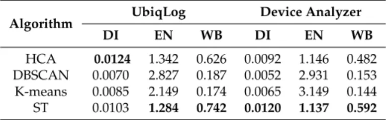
In order to measure the quality of our ST clustering algorithm, we have used the Dunn Index

(DI) [32], entropy (EN) [33] and distance comparison (WB). To calculate the WB, we have divided the

average distancewithinthe clusters to the average distancebetweenthe clusters. Table5reports data

for all users in both datasets.

Table5shows that our clustering algorithm (ST) outperforms others in WB and EN, on both

datasets. Only the DI, with the HCA algorithm in the UbiqLog dataset, returns a higher value (better) than ST. As previously stated, our clustering algorithm handles nondaily routines as weekend

behaviors. Table6compares the quality of our clustering algorithm in two modes (i.e., ST1 and ST2).

ST1 neglects the orphan events analysis in the clustering algorithm. ST2 takes into account orphan

events and thus its accuracy should be higher. Table6shows the higher accuracy in ST2 compared to

ST1 and thus demonstrates the ability of our algorithm to correctly identifying non-daily behaviors. In particular, at the first iteration of clustering 33% of events were orphan events, which do not stay in a cluster. During the next iteration, only 11% of events remained as anomalous events, and 22% were assigned to existing clusters. Calculating orphan events does not have any impact on quantitative results, including execution time and battery utilization. Its only impact is on the quality of clustering.

Table 5.Quality comparison between ST and representative clustering methods in two datasets.

Algorithm UbiqLog Device Analyzer

DI EN WB DI EN WB

HCA 0.0124 1.342 0.626 0.0092 1.146 0.482

DBSCAN 0.0070 2.827 0.187 0.0052 2.931 0.153 K-means 0.0085 2.149 0.174 0.0065 3.149 0.144 ST 0.0103 1.284 0.742 0.0120 1.137 0.592

Table 6.Comparision of the clustering approach by analyzing orphan events (ST1) and not analyzing them (ST2).

Clustering Algorithm Precision Recall F-Measure

ST1 0.78 0.72 0.75

ST2 0.81 0.74 0.78

Analysis in Tables4and5has been conducted on all 70 users. However, results of Table6require

subjective annotation. Therefore, we have conducted this experiment on 20 ground truth users and not on all users.

5.2.3. Parameter Sensitivity of Lambda

λis the configurable parameter that has been used as a boundary for identifying similar events

and clustering them together. In order to analyze the sensitivity ofλ, we report on four different values

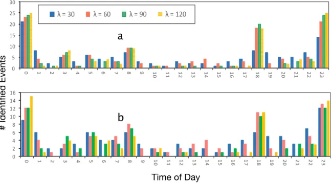
forλ: 15, 30, 60 and 90 min. Figure6reports about the number of events that have been identified in

each dataset, based on differentλvalues and time of the day (from 12:00 a.m. to 11:59 p.m.). This figure

reports on all users as well.

In particular, increasingλresults in a fewer number of clusters because of short time events,

which are neglected (less than 600or 900). However, at some specific times, a largerλcan identify more

events, which appears as spikes in Figure6. For instance,λwith large values, i.e., 600, 900and 1200,

can identify more events near bed time and commuting times. There are three main spikes in both datasets including leaving for work/school, arriving home and near bed time. The first spike, which is

bedtime around 00:000, is connected to the last spike, which started around 11:00 p.m. Therefore,

we can observe three major spikes and not four spikes.

Based on Figure6, different values ofλ(except 15 min) do not have significant differences on the

number of events. Setting lambda to 15 min leads to a fewer number of events in a cluster. Otherλ

have approximately similar results. On the other hand, the ground truth dataset users have evaluated

the precision of differentλsettings. Table7reports the WGL settings with differentλ. In particular,

30 and then 60 min have the highest accuracy, followed by 90 and 15 min. Therefore, based on the

identified accuracy in Table7, we identify that the optimal value of lambda is 30 min, followed by

60 min. Note that all routine events are not associated with 30’ temporal differences. For instance, calling a friend every day is not precise to fit into a 30’ slope. Nevertheless, there are more precise

events, such as arriving at work, which neutralizes the impact of those imprecise routine events.λis a

parameter that reports a single best estimator for all behaviors.

Results in Figure6were based on using all users’ data. However, results in Table7are from

0 2 4 6 8 10 12 14 16 0 1 2 3 4 5 6 7 8 9 10 11 12 13 14 15 16 17 18 19 20 21 22 23 0 5 10 15 20 25 30 0 1 2 3 4 5 6 7 8 9 10 11 12 13 14 15 16 17 18 19 20 21 22 23 λ = 30 λ = 60 λ = 90 λ = 120

a

b

Time of Day

# Identified Events

Figure 6. Impact of differentλvalues on the number of events detected during the day. (a) is the UbiqLog dataset and (b) is the Device Analyzer (best viewed in color).

Table 7.Accuracy of different values forλ. Lambda Values 150 300 600 900 F-Score 0.77 0.91 0.85 0.78 Precision 0.77 0.90 0.87 0.83 Recall 0.78 0.92 0.85 0.82

5.2.4. Search and Battery Impact

The cluster-based search mechanism can be understood as a one-dimensional ‘index’ that has been used to accelerate searching. Clustered data are amenable to further indexing (e.g., bitmap, B-trees, etc.), but here we confine our attention just to the improvements obtained by our re-representation of the data. As previously noted, the problem of searching sensor data has not been widely explored for mobile and wearable devices. Mobile/wearable sensing applications can collect large amounts of data; however, searching them is a resource intensive process and thus a simple brute force search on raw data is not feasible.

Since all 70 users can not annotate their data, we only use our ground truth users. Participants of the ground truth dataset manually segmented their daily events with the following words: “Commute”, “Home”, “Work”, “Leisure” and “Other”. We have implemented a Wi-Fi and location geo-fencing component to automatically replicate labels to the other events in the same cluster. Then, we assign the described labels to all 70 users (based on labels’ distribution in the time of day) by using our ground truth labels as a template, e.g., morning events are usually ‘commute’ or ‘work’, evening events are ‘Home’ or ‘Leisure’. Label assignments are not necessarily correct, but the objective here is to prepare

them for searching by disregarding their semantics.

To test searching on the labeled data, we have considered two search algorithms. One is brute force, used as a baseline, which has been compared to our clustering algorithm. These experiments

Analyzer dataset and the UbiqLog dataset. We have considered four types of search for each user sample, which includes both time and location (due to spatio-temporality of clusters):

(i) search with time (T), location state (L), sensor name (S) and sensor data (D) (Figure 7a,

e.g., How long on average do I spend playing games, while at home, after 9:00 p.m.?

(ii) search with L, S, D, Figure7b, e.g.,How many SMS do I receive, on average, while at work?

(iii) search with T, S and D Figure7c, e.g.,When was the last time I went running?

(iv) search with S, D, Figure7d, e.g.,How often did I call my parents?

To parse the user input, we have used a light query engine [34] that can parse Quantified-Self

queries on mobile and wearable devices. Numbers presented in Figure7are averaged among all

users in each dataset, i.e., they present an average user time required for queries on the smartphone.

However, Figure7d has no notion of time or location. Figure7demonstrates the significant impact of

the clustering algorithm on search execution time for both datasets. The improvement increases with the size of the data. However, query (d) that does not include either a notion of time or location does not have any significant difference with the brute force method.

0 5000 10000 15000 20000 25000 10 20 30 40 50 60 0 5000 10000 15000 20000 10 20 30 40 50 60 0 5000 10000 15000 20000 10 20 30 40 50 60 a b c 0 5000 10000 15000 20000 10 20 30 40 50 60 # days d 0 5000 10000 15000 20000 25000 10 20 30 40 50 60 Clustering Brute3 Force 0 5000 10000 15000 20000 25000 10 20 30 40 50 60 0 5000 10000 15000 20000 25000 10 20 30 40 50 60 a b c

Execution Time (millisecond)

0 5000 10000 15000 20000 25000 10 20 30 40 50 60 # days d

UbiqLog Device Analyzer

Figure 7.Four different search execution time samples for UbiqLog and Device Analyzer. They-axis shows execution time in milliseconds and thex-axis shows the number of days that will be searched.

Note that there is no space overhead, since the clustering merely changes the storage file structure. The only overhead is the time required for the cluster calculation, which can be done at off-peak times, e.g., when the device is charging. Moreover, the improvements in speed do not come at a cost of

accuracy; the search of our condensed data isadmissible, producingidenticalresults to the search over

the original raw data.

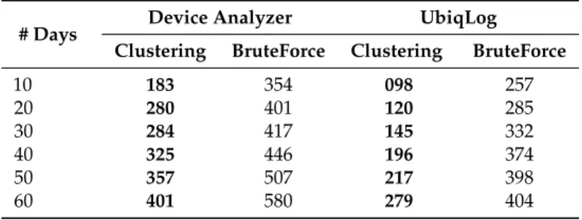
As noted previously, battery utilization is a major challenge in small devices [35]. Here, we also

demonstrate the battery utilization differences between our cluster-based search versus the brute

force search (baseline). Table8shows the impact of our cluster based search on battery efficiency,

as measured in microWatts (mW) and significant improvements over brute force search. This table reports the averaged battery utilization among all four types of aforementioned queries.

Table 8.Energy use in micro-Watt (mW) comparing brute force and our cluster based search operations.

# Days Device Analyzer UbiqLog

Clustering BruteForce Clustering BruteForce

10 183 354 098 257 20 280 401 120 285 30 284 417 145 332 40 325 446 196 374 50 357 507 217 398 60 401 580 279 404

5.3. Contrast Behaviors

Three experiments have been used to evaluate our Contrast Behavior (CB) detection approach.

First, the parameter sensitivity ofω and its impact on the quantity of CBs was analyzed. Second,

characteristics of CBs were determined by analyzing the correlation between time of the day and event duration. The third experiment examined the search execution time based on prioritizing clusters ordered by their number of CBs.

5.3.1. Parameter Sensitivity of Omega

It is notable that the Device Analyzer dataset contains only hardware configuration or changes in the hardware properties, thus its data objects are not necessarily correlated with human behaviors.

Therefore, the second evaluation used the UbiqLog dataset (35 users).ωis a configurable parameter

we have introduced to be used for CB identification. Similar to that for other clustering algorithms,

such as K-means, there can not be an optimal value for ω. This variable is open to settings by

developers using this algorithm. For instance, a user might frequently go to a coffee shop in the evenings (similar spatio-temporal event, assigned to the same cluster) either for work, or chatting with friends. Both scenarios take place in the coffee shop at about the same time, but her other actions could be different. If the goal of the target application is to detect only appearances in the coffee shop,

and not other actions,ωcould be set to zero. However, if the goal of the target application is to detect

reasons for being in a coffee shop,ωshould be set to more than zero, to detect dissimilar actions.

As another example, a user either goes bird watching or golfing to a golf course. These activities could

be identified via a comparison between wrist movement data, in which caseωcan be equal to one.

To gain a deeper understanding about the events inside each cluster, we have tested five different

variables forω: 1,2,3,4 and 5. Figure8a reports about the number of detected events among all users

in the UbiqLog dataset and Figure8b reports on the Device Analyzer dataset. As it has been shown,

increasing the value ofωdecreases the number of similar events, thus resulting in more events from

each cluster being considered as CBs. Figure8shows that the boundary for settingω is different

between two datasets. For instance, settingωto three and larger creates more CBs than similar events,

in the Device Analyzer dataset. Nevertheless,ωis not dataset dependent, increasing it simply reduces

the chance of having more similar entities and vice versa.

85 74 ₇₁ 68 35 51 54 57 0 20 40 60 80 100 1 2 3 4 Similar0Events Contrast0Behaviors ₁₀₂ 96 ₉₂ 84 73 84 88 92 0 20 40 60 80 100 120 1 2 3 4

#

a

_b

Figure 8.Parameter sensitivity ofωin (a) UbiqLog dataset and (b) Device Analyzer dataset.

5.3.2. Characteristics of Contrasting Events

Our CB identification algorithm is capable of identifying dissimilar actions for routine behaviors. We begin with the observation that for most people, their range of behaviors is very limited between 12:00 a.m.–8:00 a.m. (while sleeping), more varied between 8:00 a.m.–4:00 p.m. (during work or school) and highly varied after 4:00 p.m. (during leisure time). To show this, we use an approach similar

and 4:00 p.m.–11:59 p.m. We consider only events shorter than 16 h. Figure9b which is done for

ω= 3, shows the average distribution of the ratio between similar and dissimilar actions belonging

to events from a single cluster. Morning events have the fewest number of CBs, perhaps because behaviors following sleep tends to be routine. In contrast, evening events have a higher number of CBs, supporting our initial hypothesis.

0 200 400 600 800 1000 0.00 3.00 6.00 9.00 12.00 15.00 0 200 400 600 800 1000 0.00 3.00 6.00 9.00 12.00 15.00 Event Duration # Actions

a

b

c

Figure 9.(a) distribution of similar actions (not events); (b) distribution of dissimilar actions; both (a,b) were based on event duration usingω=3; (c) ratio of similar actions inside events of each cluster, distributed among different temporal segments.

In order to evaluate these findings, we have created a contingency table of temporal segments

(8 h and 16 h segments) and dissimilar and similar actions. Similar to [13], we use the chi-square test

to statistically evaluate our interpretation. The result (p<0.05) supports our assumptions about the

distribution of contrasting behaviors among different temporal segments.

Another interesting finding (Figure9a) shows that the distribution of dissimilar actions is highly

concentrated on short temporal events. In contrast, events longer than three hours have far fewer dissimilar actions. This maps to our intuition that routine spatio-temporal behaviors are longer by their nature, e.g., staying 9 h at work, sleeping 7 h per day, etc. To validate this observation, we have calculated the odds ratio of the number of similar actions versus dissimilar actions, and the number of actions, which have less than three versus more than three hours duration. The result of the odds ratio calculation indicates clusters that last less than three hours are 8.2 times more likely to have contrasting behaviors than clusters with events longer than three hours.

5.3.3. Contrast Behavior Impact on Search

Understanding the characteristics of contrasting behaviors could improve the search execution time by prioritizing clusters, i.e., first, the system searches clusters with a lower number of CBs and then searches clusters with a higher number of CBs. In order to evaluate this hypothesis, we have ordered the clusters based on the number of their CB ratio to similar events, i.e., a cluster with a higher number of CBs gets a lower rank. There is a small cost of ordering clusters, but, due to the small

number of clusters, it is insignificant. In Section5.2.4, we execute two different search commands for

each of the described search conditions. The first search command gets the data from the cluster with the largest number of CBs, and the second command, in contrast to the first one, gets the data from the cluster with the highest number of similar events.

Figure10shows the differences between searching clusters ordered by number of CBs versus not ordered. As it has been shown, there is a slight improvement in the search execution time, especially when the number of days increases. This result is in line with our initial hypothesis, and thus ordering clusters based on their CBs can reduce the search execution time.

0 1000 2000 3000 4000 5000 10 20 30 40 50 60 Ordered,Cluster not,Ordered 0 1000 2000 3000 4000 5000 10 20 30 40 50 60

Execution Time (millisecond)

#days

a

b

Figure 10.Improvement of search execution time (in milliseconds) by ranking clusters based on their number of contrast behaviors. (a) UbiqLog and (b) Device Analyzer dataset.

6. Related Work

Based on our contributions reported in this paper, we categorize related works into three different categories. First, we review works that focus on spatio-temporal segmentation or clustering from mobile devices and their sensors, i.e., WiFi, GPS and Cell ID. Then, we review works that focus on detecting patterns of location changes or location of interests. Afterward, we review works that try to extract events from daily life events. These works either rely on sensor data or are user-centric and focus on daily activities of users. There are several works that attempt to estimate users’ behavior from cell tower data, but since our approach is focused on data from users‘ devices, we do not list

them here. For example, Ghahramani et al. [37] focuses on identifying geographical hotspots based

on smartphone concentrations, by analyzing spatial information of cell IDs collected from a telecom provider. In addition, there are some works that employ other mediums for location information

mining, such as social media [38], which we do not list them here.

6.1. Spatio-Temporal Segmentation

Zhou et al. [26] provide one of the earliest works in spatio-temporal clustering of daily location

changes. To address sparse and noisy GPS data, they provide a density-based algorithm for clustering because density based algorithms can remove noise in the final clustering results. There are several

works that have focused on geographical location. For instance, Mokbel et al. [39] propose a

three-phase algorithm (hashing, invalidating and joining) to parse continuous spatio-temporal queries.

Zhang et al. [40] use text as a raw material for location with an index structure that reduces the search

space using spatial and keyword base pruning. A recent example is introduced by Christensen et al. [41]

which focuses on facilitating accessing spatio-temporal through interactive spatial online sampling

techniques. There are other indexing methods that operate on multi-metric characteristics of data [42],

such as location or time. However, our work uses spatio-temporal similarity of data for indexing.

6.2. Location and Spatial Information Mining

There are several examples of research that benefit from smartphone location logs, i.e., GPS, WiFi,

Cell ID, to identify locations of interest and daily movement patterns. Reality mining [16], is one of the

first efforts toward identifying behavior from smartphone sensor data and so created a benchmark

dataset that is still in use, e.g. [14]. For instance, Farrahi et al. [14] use distant n-gram topic modeling

to mine latent location data and avoid parameter dimension explosion. Recently, the uncertainty of a realistic deployment has been taken into account and there are some works that try to support