Abstract—It is challenging to acquire satellite sensor data with both fine spatial and fine temporal resolution, especially for monitoring at global scales. Amongst the widely used global monitoring satellite sensors, Landsat data have a coarse temporal resolution, but fine spatial resolution, while MODIS data have fine temporal resolution, but coarse spatial resolution. One solution to this problem is to blend the two types of data using spatio-temporal fusion, creating images with both fine temporal and fine spatial resolution. However, reliable geometric registration of images acquired by different sensors is a prerequisite of spatio-temporal fusion. Due to the potentially large differences between the spatial resolutions of the images to be fused, the geometric registration process always contains some degree of uncertainty. This paper analyzes quantitatively the influence of geometric registration error on spatio-temporal fusion. The relationship between registration error and the accuracy of fusion was investigated under the influence of different temporal distances between images, different spatial patterns within the images and using different methods (i.e., spatial and temporal adaptive reflectance fusion model (STARFM) and Fit-FC; two typical spatio-temporal fusion methods). The results show that registration error has a significant impact on the accuracy of spatio-temporal fusion: as the registration error increased, the accuracy decreased monotonically. The effect of registration error in a heterogeneous region was greater than that in a homogeneous region. Moreover, the accuracy of fusion was not dependent on the temporal distance between images to be fused, but rather on their statistical correlation. Finally, the Fit-FC method was found to be more accurate than the STARFM method, under all registration error scenarios.
Index Terms—Remote sensing data, Landsat, MODIS, spatio-temporal fusion, registration error.
I. INTRODUCTION
In recent years remote sensing has developed rapidly and has been applied widely, for example, in land use and land cover Manuscript received November 13, 2019; accepted 6 January, 2020. This work was supported by National Natural Science Foundation of China under Grant 41971297, Tongji University under Grants 0250141304 and 02502350047, and the Project Supported by the Open Fund of Key Laboratory of Urban Natural Resources Monitoring and Simulation, Ministry of Natural Resources under the Grant KF-2019-04-003 (Corresponding author: Qunming Wang.).
Y. Tang and Q. Wang are with the College of Surveying and Geo-Informatics, Tongji University, 1239 Siping Road, Shanghai 200092, China (e-mail: [email protected]).
K. Zhang is with the School of Geography and also with Jiangsu Center for Collaborative Innovation in Geographical Information Resource Development and Application, Nanjing Normal University, 1 Wenyuan Road, Nanjing 210023, China.
P.M. Atkinson is with the Faculty of Science and Technology, Lancaster University, Lancaster LA1 4YR, UK; School of Geography, Archaeology and Palaeoecology, Queen’s University Belfast, BT7 1NN, Northern Ireland, UK; Geography and Environment, University of Southampton, Highfield, Southampton SO17 1BJ, UK; State Key Laboratory of Resources and Environmental Information System, Institute of Geographical Sciences and Natural Resources Research, Chinese Academy of Sciences, Datun Road, Beijing 100101, China.
change monitoring [1], vegetation monitoring [2], carbon sequestration monitoring [3], revealing ecosystem climate feedbacks [4], evaluating forest and ecological environments [5], and urban monitoring [6]. With rapid changes on the Earth’s surface, it is becoming increasingly important to perform monitoring at finer spatial and temporal resolutions. Such fine resolution monitoring sometimes cannot be performed with a single sensor due to the trade-off between spatial and temporal resolution. Spatio-temporal fusion is one solution to this problem, which creates time-series images with fine temporal
and spatial resolutions by blending images with fine temporal resolution (e.g., MODIS) and fine spatial resolution (e.g., Landsat) through computer processing. Great progress has been achieved in developing spatio-temporal fusion techniques [7], which can be divided into two main groups: weighting function-based and spatial unmixing-based methods.
The basic principle of weighting function-based methods is to calculate the reflectance of the center fusion pixel through a weighting function which takes full account of the spectral, temporal and spatial information in similar pixels. Such methods have been used widely. Gao et al. [8] proposed the spatial and temporal adaptive reflectance fusion model (STARFM), which includes comprehensive consideration of the spectral difference between MODIS and Landsat ETM+ data, the temporal difference between MODIS data of the same pixel location, and the distance between the center pixel and similar pixels. Thus, different weights are applied to different pixels to predict the reflectance of the center pixel. Hilker et al. [9] proposed the spatial temporal adaptive algorithm for mapping reflectance change (STAARCH) to solve the problem of rapid land cover change that is not resolved by STARFM. Tasseled cap transform results were introduced to calculate the change sequence, which can increase the prediction accuracy effectively. To deal with low accuracy in heterogeneous regions, Zhu et al. [10] proposed the enhanced spatial and temporal adaptive reflectance fusion model (ESTARFM). The hypothesis made was that there is a linear relationship between the changes in the MODIS and Landsat reflectances during a given period. A conversion coefficient was introduced to express this relationship quantitatively, which ensures more accurate prediction of the reflectance of small and linear targets. Wang and Atkinson [11] proposed the Fit-FC model, which realizes spatio-temporal fusion through three steps; regression model fitting (RM fitting) spatial filtering (SF) and residual compensation (RC). It was found that the accuracy of the algorithm was greater than all the comparator methods, and the model can be implemented with only one pair of coarse-fine images. Weighting function-based methods can also be applied to predict land surface temperature with both fine spatial and temporal resolution [12].
Spatial unmixing-based methods calculate the reflectance of corresponding classes at the fine spatial resolution by unmixing
pixels in the coarse spatial resolution image, where the coarse proportions are available (i.e., simulated from temporally close fine spatial resolution data) [13]. This is in contrast to the well-known spectral unmixing technique where the reflectance of class is known and the target is to predict coarse proportions. Zhukov et al. [14] developed a multisensor multiresolution technique (MMT). The first step of MMT is to classify the fine resolution image and upscale the thematic map to the coarse spatial resolution, such that the proportions of each class in each of the coarse pixels can be calculated. Then, the reflectance of each class is estimated by fitting a model using the coarse reflectance in a local window. Considering the variation of reflectance within a specific class, Maselli et al. [15] proposed a LAC-GAC NDVI integration method. It corrects pixels whose residuals exceed a certain threshold among all neighboring pixels. The weight of each neighboring pixel is calculated according to their distance to the center pixel to be corrected. However, abrupt changes in reflectance between neighboring pixels always cause uncertainty. To cope with this problem, Busetto et al. [16] took the spectral similarity and Euclidean distance between neighboring pixels and the target pixel into consideration simultaneously when correcting the target pixel. Specifically, spectral similarity between pixels was calculated using spectral information in fine spatial resolution images, to split out pixels that are spatially close to the target pixel, but spectrally far from the target pixel. Wu et al. [17] proposed a spatial-temporal data fusion approach (STDFA) to cope with the heterogeneity of the ground object distribution. STDFA accounts for the spectral difference between pixels of the same land cover class and also the non-linear temporal change in the reflectance of each class over a period. This method used the surface reflectance calculation model (SRCM) to calculate the reflectance change of each fine pixel during the time of interest. The final prediction is the combination of the reflectance of the fine spatial resolution pixels at the known time and the reflectance change over the period. Wu et al. [18] then proposed the Modified Spatial and Temporal Data Fusion Approach (MSTDFA) method to increase the accuracy of STDFA by correcting for sensor differences and introducing an adaptive window size.
The Flexible Spatiotemporal DAta Fusion (FSDAF) method proposed by Zhu et al. [19] combines the advantages of unmixing-based and weighting function-based methods. Liu et al. [20] proposed an Improved Flexible Spatiotemporal DAta Fusion (IFSDAF) method, which employs information from multi-time predictions, making full use of all available images. Besides the above two main groups of methods, learning-based and Bayesian-based methods have also been developed for spatio-temporal fusion. The SParse-representation-based SpatioTemporal reflectance Fusion Model (SPSTFM) proposed by Huang [21] selects plenty of patches for dictionary-pair learning and, thus, the correspondence between the coarse and fine spatial resolution images can be established. Song and Huang [22] developed a method using only one pair of coarse and fine images for prediction. In this method, the sparse representation is utilized to realize the super-resolution of fine temporal resolution images and a high-pass modulation is applied for fusion. Wei et al. [23] included prior knowledge to increase the accuracy of the sparse representation-based method. This method builds a model containing semi-coupled dictionary
learning and structural sparsity. Recently, some learning-based methods applying deep convolutional neural networks (CNN) have also been developed. The method proposed by Song et al.
[24] established two five-layer CNNs to achieve spatio-temporal fusion. As for Bayesian-based methods, Bayesian estimation theory was applied to spatio-temporal fusion [25]. Moreover, based on nonlinear geostatistical theory, Bayesian Maximum Entropy (BME) [26] was also developed to fuse data acquired by different sensors.
No matter which spatio-temporal fusion method is adopted, reliable geometric registration of the images acquired by different sensors is a prerequisite. However, there exist unavoidable differences between the coarse (e.g., MODIS) and fine spatial resolution (e.g., Landsat) time-series images to be fused that make registration challenging [27]. The most obvious challenge is due to spatial resolution (e.g., zoom factor of around 16 between Landsat and MODIS images). Moreover, additional factors exist, for example, differences in sensor characteristics and the Bidirectional Reflectance Distribution Function (BRDF) effect due to differences in viewing angles, Sun elevation and atmospheric conditions at the time of imaging. Furthermore, owing to the different observation scales, images acquired from various satellite sensors may also differ in projection distortion, especially for the pixels at the edge of the acquisition. The pre-processing of reprojection of images contributes to the registration error to a great extent. Thus, the geometric registration process for two or more types of observations always contains large uncertainty.
Recent studies showed that geometric registration error has a significant influence on land cover classification and change detection [28]-[33]. Furthermore, in recent reviews of the literature on spatio-temporal fusion, it was acknowledged that the registration error between multi-source images plays an important role in spatio-temporal fusion, and it remains an open problem [34]-[37]. To the best of our knowledge, however, very few studies have focused on the extent to which geometric registration error can affect spatio-temporal fusion results. Based on existing typical and accurate spatio-temporal fusion methods (i.e., STARFM [8] and Fit-FC [11]), this paper investigated the influence of registration error between MODIS and Landsat images on spatio-temporal fusion under the conditions of varying temporal distance, spatial patterns and methods. Note that the spatial unmixing-based methods were not considered in this paper. The reason is that this type of methods assumes that within a coarse pixel, all pixels of the same land cover class share the same reflectance. Thus, the method cannot reproduce the intra-spectral variation. Moreover, it always results in visually obvious blocky artifacts.
The remainder of this paper is organized into four sections. Section II quantifies the uncertainty of MODIS data due to registration error and briefly introduces two spatio-temporal fusion methods, STARFM and Fit-FC. Section III introduces the data including the simulation of MODIS data with registration errors. Then, the experimental results are provided, including the quantitative analysis of the influence of registration error on spatio-temporal fusion, and the influences of temporal distance, spatial patterns and methods. Section IV further discusses the findings from the experiments and potential future research, followed by a conclusion in Section V.
y
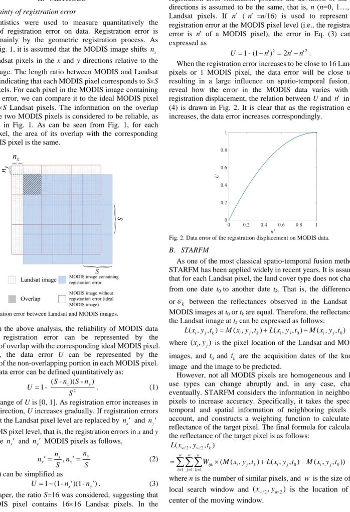
Landsat image. The length ratio between MODIS and Landsat pixels is S, indicating that each MODIS pixel corresponds to SS
Landsat pixels. For each pixel in the MODIS image containing registration error, we can compare it to the ideal MODIS pixel covering SS Landsat pixels. The information on the overlap between the two MODIS pixels is considered to be reliable, as represented in Fig. 1. As can be seen from Fig. 1, for each MODIS pixel, the area of its overlap with the corresponding ideal MODIS pixel is the same.
Fig. 1. Registration error between Landsat and MODIS images.
Based on the above analysis, the reliability of MODIS data containing registration error can be represented by the proportion of overlap with the corresponding ideal MODIS pixel. Meanwhile, the data error U can be represented by the proportion of the non-overlapping portion in each MODIS pixel. Thus, the data error can be defined quantitatively as:
2 ( )( ) 1 S - nx S - ny U - S . (1) The value range of U is [0, 1]. As registration error increases in the x or y direction, U increases gradually. If registration errors
x
n andny at the Landsat pixel level are replaced by nx and ny at the MODIS pixel level, that is, the registration errors in x and y
direction are nx and ny MODIS pixels as follows,
, y x x y n n n n S S (2) then Eq. (1) can be simplified as
1 (1 x)(1 y)
U - n - n . (3) In this paper, the ratio S=16 was considered, suggesting that each MODIS pixel contains 1616 Landsat pixels. In the
When the registration error increases to be close to 16 Landsat pixels or 1 MODIS pixel, the data error will be close to 1, resulting in a large influence on spatio-temporal fusion. To reveal how the error in the MODIS data varies with the registration displacement, the relation between U and n in Eq. (4) is drawn in Fig. 2. It is clear that as the registration error increases, the data error increases correspondingly.
Fig. 2. Data error of the registration displacement on MODIS data.
B. STARFM
As one of the most classical spatio-temporal fusion methods, STARFM has been applied widely in recent years. It is assumed that for each Landsat pixel, the land cover type does not change from one date t0 to another date tk. That is, the difference
0or
k between the reflectances observed in the Landsat and MODIS images at t0 or tk are equal. Therefore, the reflectance of the Landsat image at tk can be expressed as follows:0 0
( ,i j, )k ( ,i j, )k ( ,i j, ) ( ,i j, ) L x y t M x y t L x y t M x y t (5) where ( ,x yi j) is the pixel location of the Landsat and MODIS images, and
t
0 andt
k are the acquisition dates of the known image and the image to be predicted.However, not all MODIS pixels are homogeneous and land use types can change abruptly and, in any case, change eventually. STARFM considers the information in neighboring pixels to increase accuracy. Specifically, it takes the spectral, temporal and spatial information of neighboring pixels into account, and constructs a weighting function to calculate the reflectance of the target pixel. The final formula for calculating the reflectance of the target pixel is as follows:
/ 2 / 2 0 0 1 1 1 ( , , ) ( ( , , ) ( , , ) ( , , )) w w k w w n ijk i j k i j i j i j k L x y t W M x y t L x y t M x y t
(6)
where n is the number of similar pixels, and
w
is the size of the local search window and(
x
w/ 2,
y
w/ 2)
is the location of the center of the moving window.The performance of STARFM depends greatly on the size of the characteristic patch, the spatial heterogeneity of the region, and more importantly, the magnitude of the land cover changes in the temporal domain.
C. Fit-FC
The Fit-FC method was proposed as a response to several problems faced in practical situations such as the difficulty in obtaining sufficient, high-quality images on dates close to the date to be predicted and strong phenological changes between the known and prediction dates. A local regression model is used to enhance the connection between the coarse image on the known date and the date to be predicted, thus, increasing the accuracy of the prediction. The methodology of Fit-FC is divided into three main steps; regression model fitting (RM fitting), spatial filtering (SF) and residual compensation (RC).
1) RM fitting. Regression model fitting is performed based on the local spatial variation in land cover. In a local window, the coarse band pixel reflectances acquired on different dates are expressed as a linear relationship. The moving window is applied to all pixels and all coarse bands. This coefficient set calculated from the regression model constructed for the coarse data can be applied to fine spatial resolution images to obtain the initial prediction result, as shown in Eq. (7):
RM ( 0, ) ( , )b 1 0 b ( 0, )b
F a X l F x l b X l . (7) In Eq. (7),
x
0 is the location of the center Landsat pixel of the window, and X0 is the location of the center MODIS pixelwhere
x
0 falls withinX0 . a X l( 0, )b and b X l( 0, )b are local linear regression coefficients estimated based on the regression model constructed for the MODIS data, and F x l1( 0, )b is the reflectance of the Landsat pixel located atx
0 in band lb of theknown fine spatial resolution image.
2) SF. To reduce the brick effect in the prediction of the first step, a spatial filter is used where different weights are assigned to neighboring pixels to correct the reflectance of the center pixel, as shown in Eq. (8):
SF 0 RM 1 ( , ) ( , ) m b i i b i F x l W F x l
. (8) In Eq. (8), m is the number of similar pixels, Wi is the weight, andFRM( , )x li b is the result of step 1.3) RC. Residuals inevitably exist in the regression model, and need to be considered in the final prediction results. Based on the assumption that similar pixels share similar residuals, the residuals of the center pixel can be corrected using the residuals of neighboring pixels. The calculation is in the same way as that in Eq. (8).
The final prediction is the sum of the above SF and RC predictions. Fit-FC can be conducted using only one pair of MODIS-Landsat images, and is especially suitable where strong phenological changes exist.
D. Accuracy evaluation indices
Quantitative evaluation was conducted using the indices of Root Mean Square Error (RMSE), Correlation Coefficient (CC) and Universal Image Quality Index (UIQI). They were calculated for each band separately and the values for all bands
were then averaged. The calculation for a single band image is introduced below.
(1) Root Mean Square Error (RMSE)
RMSE measures the difference between the fusion image and the reference image [39], and its ideal value is 0. That is, the smaller the RMSE, the more accurate the prediction. RMSE is defined as ( , ) ( , ) 1 1 1 M N i j i j i j RMSE MN
F X (9) where F and X represent the fusion prediction and reference image (with the same spatial size of MN), respectively.Reflectance varies in magnitude across bands. To reduce the influence of the magnitude of reflectance, it is more appropriate to use the Relative Root Mean Square Error (RRMSE) [40]. RRMSE is defined as
( , )i j
RMSE RRMSE
X (10) where X( , )i j is the mean value of the reflectance of the reference image.
(2) Correlation Coefficient (CC)
CC is an objective evaluation index reflecting the correlation between the fusion image and the reference image [41]. The ideal value is 1. The more similar the two images, the closer the CC is to 1. CC is defined as ( , ) ( , ) 1 1 2 2 ( , ) ( , ) 1 1 1 1 M N i j F i j X i j M N M N i j F i j X i j i j CC
F X F X (11)where
F and
X represent the mean values of F and X. (3) Universal Image Quality Index (UIQI)The UIQI proposed by Wang et al. [42] was applied to evaluate the similarity between the fusion image and the reference image. The closer the UIQI is to 1, the more accurate the prediction. UIQI is defined as
2 2 2 2
2
2
FX F X F X F X F X F XUIQI
(12)where
FX represents the covariance between F and X, and F
and
X are the standard deviations of F and X.III. EXPERIMENTAL RESULTS
A. Data
Two datasets were used in this paper. The first dataset covers an irrigation area in Coleambally, New South Wales, Australia (called Region 1 hereafter), while the second dataset covers the southern research area of the Boreal Ecosystem-Atmosphere Study (BOREAS) with short growing season and extreme phenological changes (called Region 2 hereafter). Four Landsat 8 OLI images with a spatial size of 942942 pixels were used for Region 1. The Landsat images contain six bands (blue, green, red, NIR, SWR1 and SWR2 bands). For Region 2, three Landsat 7 ETM+ images with a spatial size of 815815 pixels were used. As shared by Gao et al. [8], the images contain three bands,
(a) (b) (c) (d)
(e) (f) (g) (h)
Fig. 3. Region 1 data (NIR, red, and green bands as RGB). (a)-(d) are Landsat images at t1, t2, t3 and t4, respectively. (e)-(h) are the corresponding MODIS images.
(a) (b) (c)
(d) (e) (f)
Fig. 4. Region 2 data (NIR, red, and green bands as RGB). (a)-(c) are Landsat images at t1, t2, and t3, respectively. (d)-(f) are the corresponding MODIS images.
Table 1 Summary of the experimental data
Region Acquisition date
Region 1 t1: 2013.07.06 t2: 2013.08.14 t3: 2013.09.08 t4: 2013.11.18 Region 2 t1: 2001.05.24 t2: 2001.07.11 t3: 2001.08.12
(including green, red and NIR bands). Table 1 lists the properties of the images.
Among the set of images, we chose the Landsat data at t1 in
Regions 1 and 2 as the known image with which to predict the Landsat images on the other dates in the two regions. The Regions 1 and 2 data are shown in Figs. 3 and 4, respectively. It is seen that the two regions differ significantly in spatial variation. The local spatial heterogeneity in Region 1 is visually greater than that in Region 2, where spatial heterogeneity refers to the spatial complexity and variability of the system or system
attributes [38].
B. Experimental setup
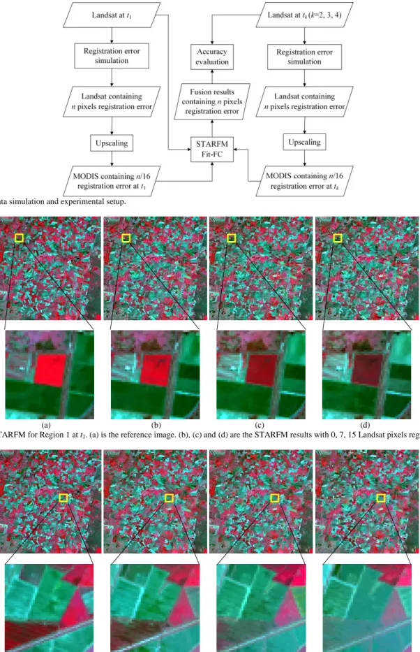
Fig. 5 shows the methodology and experimental design. It should be stressed that we simulated MODIS data that have a registration error with Landsat data, as this allows greater control on the analysis of the performance where the registration error and reference are known perfectly. Specifically, based on the Landsat images at t1 and tk(k=2, 3, 4), Landsat images with n (n=0, 1…, 15) pixels registration error were produced by
registration error simulation. That is, the simulated images were produced by shifting n Landsat pixels both horizontally and vertically. MODIS images on two dates were then synthesized by upscaling the Landsat images (the ratio is 16, i.e., each block of 16 by 16 Landsat pixels was aggregated to a MODIS pixel) with registration error on two dates. Fig. 3(e)-(h) and Fig. 4(d)-(f) show the simulated MODIS data without registration error for Regions 1 and 2, respectively. STARFM and Fit-FC were
Fig. 5. Process of data simulation and experimental setup.
(a) (b) (c) (d)
Fig. 6. Results of STARFM for Region 1 at t2. (a) is the reference image. (b), (c) and (d) are the STARFM results with 0, 7, 15 Landsat pixels registration error.
(a) (b) (c) (d)
Fig. 7. Results of Fit-FC for Region 1 at t2. (a) is the reference image. (b), (c) and (d) are the Fit-FC results with 0, 7, 15 Landsat pixels registration error.
implemented to fuse the Landsat and MODIS (containing registration error) images at t1, and MODIS image (containing
registration error) at tk. The fusion results under the condition of
n Landsat pixel(s) registration error were produced, and the accuracy was evaluated by comparing with the real Landsat image at tk. Note that the case of n Landsat pixels registration
(a) (b)
(c) (d)
(e) (f)
Fig. 8. Accuracy evaluation of the STARFM and Fit-FC predictions for Region 1 at t2. (a), (c) and (e) are RRMSE, CC, UIQI, respectively, of the STARFM result. (b), (d) and (f) are RRMSE, CC, UIQI, respectively, of the Fit-FC result.
error is equivalent to n/16 MODIS pixel registration error (at sub-pixel level relative to a MODIS pixel). Only sub-pixel level misregistration errors were considered in this paper as reported misregistration errors are typically one-pixel or less [31].
Five sub-sections (Sections III-C-G) are included in the remainder of Section III. Sections III-C and III-D provide the predictions (taking the predictions at t2 as an example) and
quantitative assessment results for Regions 1 and 2, respectively.
SectionsIII-E-G analyzes the influences of three factors on the prediction accuracy of spatio-temporal fusion. Specifically, Section III-E focuses on the influence of temporal distance. SectionIII-F defines a metric to quantify the heterogeneity of spatial patterns and discusses its impact on spatio-temporal
fusion. Section III-G investigates the differences in prediction accuracy caused by different methods.
C. Region 1
The STARFM and Fit-FC methods were implemented to predict Landsat images at t2, t3, and t4 for Region 1. The
prediction of the Landsat image at t2 was taken as an example for
detailed description. STARFM and Fit-FC were applied to fuse the Landsat and MODIS (containing registration error) images at
t1, and MODIS image (containing registration error) at t2. The
STARFM predictions of the Landsat images at t2 and the
corresponding subareas are shown in Fig. 6. With an increase in the registration error, the hue of the red target at the center of the first sub-area changes gradually. Specifically, the target in the
(a) (b) (c) (d) (e)
Fig. 9. Results of STARFM and Fit-FC for Region 2 at t2. (a) is the reference image. (b) and (c) are the STARFM results produced with 0 and 15 Landsat pixels registration error. (d) and (e) are the Fit-FC results produced with 0 and 15 Landsat pixels registration error.
Table 2 The CC between the image at the known time (i.e., t1) and prediction time (i.e., t2,t3or t4)
t2 t3 t4 Region 1 Blue 0.7969 0.5051 -0.0615 Green 0.7502 0.4464 0.1130 Red 0.7659 0.4756 -0.0524 NIR 0.7952 0.5813 0.3601 SWR1 0.7135 0.4444 0.1293 SWR2 0.6965 0.4970 0.1415 Mean 0.7531 0.4916 0.1050 Region 2 Green 0.7036 0.7735 Red 0.6828 0.7182 NIR 0.7823 0.7913 Mean 0.7229 0.7610
reference image is bright red, and the STARFM result is relatively similar to the reference image when there is no registration error. When the registration error increases to 15 Landsat pixels, however, the target turns to be dark red, which deviates greatly from the reference. The Fit-FC predictions at t2
for another area are shown in Fig. 7. It can still be noticed that with an increase in image registration error, the hue of the two triangle targets changes gradually. The color of the reference image is magenta and dark red. The color fades gradually as the registration error increases. When the registration error increases to 15 Landsat pixels, the color is quite different from the reference.
From the visual perspective, with an increase in registration error, the difference between the fusion image and the reference image increases. As shown in Fig. 8, three indices were used to evaluate quantitatively the accuracy of the fusion predictions. The conclusion is consistent with that drawn from visual analysis. That is, the accuracy decreases obviously when the registration error increases. Moreover, the accuracy changes for all six bands, which share the same trend. Taking the red band as an example, when the registration error increases from 0 to 15 Landsat pixels, the RRMSE predicted by STARFM increases by 0.0800 from 0.2277 to 0.3077. The CC decreases from 0.8772 to 0.7810 and the UIQI decreases by 0.0923.
D. Region 2
STARFM and Fit-FC were implemented for Region 2. Fig. 9 is the prediction at t2 for both methods under different
registration errors. By intra-comparison, no matter whether STARFM or Fit-FC was applied, as the registration error changes from 0 to 15 Landsat pixels, the fusion results change accordingly. The white patch in the STARFM result expands gradually, as for the pink patch in the Fit-FC result.
Quantitative evaluation of the fusion results for Region 2 at t2
is shown in Fig. 10. It is clear that the accuracy for all three bands decreases when the registration error increases. For example, for the NIR band, with the registration error increasing from 0 to 15 Landsat pixels, the RRMSE of STARFM and Fit-FC increases by 0.0138 and 0.0120, respectively. The CC and UIQI decrease by 0.0400 and 0.5140 for STARFM, and 0.0333 and 0.0349 for Fit-FC.
E. The influence of temporal distance
Intuitively, the spatio-temporal fusion prediction will be more accurate if the temporal distance between the prediction time and the known time is smaller. To test this, the accuracies of STARFM and Fit-FC were evaluated according to different temporal distances, and the results are shown in Fig. 11. The temporal distances between t2, t3, t4 and t1 are 39, 64, 135 days,
respectively. No matter which method was used, the RMSE, CC and UIQI at t2 are closer to the ideal value, revealing more
accurate prediction.
For Region 2, the same method was applied for the comparison of fusion results of different dates, as shown in Fig. 12. The temporal distance between t2 and t1 is 48 days, while that
(a) (b)
(c) (d)
(e) (f)
Fig. 10. Accuracy evaluation of STARFM and Fit-FC for Region 2 at t2. (a), (c) and (e) are RRMSE, CC, UIQI of the STARFM result. (b), (d) and (f) are RRMSE, CC, UIQI of the Fit-FC result.
STARFM or Fit-FC, the fusion result at t3 is more accurate on
the contrary. It can be concluded that the accuracy of fusion is not directly related to the temporal distance between the dates of the prediction and the known image.
To further investigate the factors affecting the predictions at different times, we compared the relations between the Landsat data at known and prediction times statistically. The CC between the image at the known and prediction time for the two regions is listed in Table 2. As can be seen from Table 2, the CC decreases from t2 to t4 for Region 1. The CC of t2 is the closest to the ideal
value, and correspondingly, the prediction of t2 is the most
accurate among the three periods. For Region 2, although the temporal distance between t3 and t1 is physically longer, the
statistical correlation between the images on the two dates is
greater, resulting in more accurate prediction. Therefore, the accuracy of spatio-temporal fusion is not related directly to the temporal distance between the prediction and known time, but to the correlation between the two images instead which can be quantified statistically. For either STARFM or Fit-FC, no matter how the registration error changes, the prediction accuracy will be greater when the correlation between the images on the two dates is greater.
F. The influence of spatial patterns
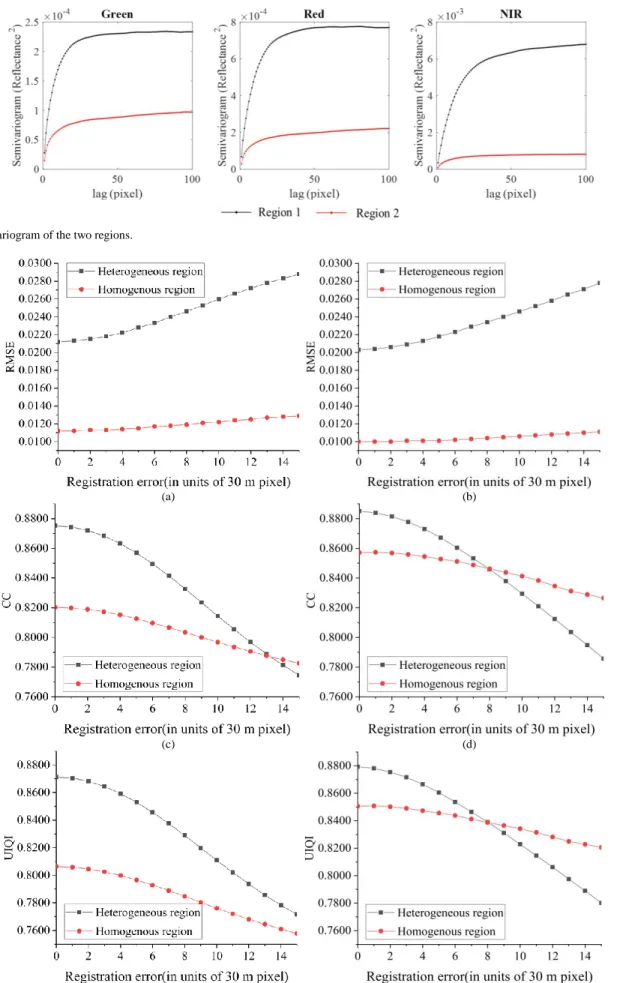
The spatial patterns of the two studied regions were characterized using the semivariogram. Specifically, the semivariograms of the green, red and NIR bands of the two known images (images at t1) were calculated. The lag varies
(a) (b)
(c) (d)
(e) (f)
Fig. 11. Accuracy evaluation result for different temporal distance in Region 1. (a), (c) and (e) are RMSE, CC, UIQI of the STARFM result. (b), (d) and (f) are RMSE, CC, UIQI of the Fit-FC result.
Table 3 The variances of the two regions, the unit of variance is 10-4 (the square of the surface reflectance)
Green Red NIR
Region 1 2.38 8.07 70.21
Region 2 1.05 2.48 8.65
from 0 to 100 Landsat pixels. The results for the three bands in the two regions are shown in Fig. 13.
It is obvious that the overall semivariogram of Region 1 is larger than that of Region 2, indicating that there is greater local variance and greater local heterogeneity in reflectance in Region 1. Meanwhile, the sample variances of the corresponding bands in the two regions were calculated to quantify the magnitude of variation, as shown in Table 3.
The sample variance of the image in Region 1 is much larger than that of Region 2, especially for the NIR band, which is as to be expected given the semivariograms. To investigate how the spatial pattern affects the accuracy of spatio-temporal fusion when registration error exists, it is necessary to fix other factors such as temporal distance between the known and prediction times. The above analysis of the influence of temporal distance showed that the correlation between the images on two dates can influence the image fusion results. Therefore, to exclude the influence of temporal distance, we selected images in the two regions that had similar between-date correlations. The mean CC of the green, red and NIR band at t2 is 0.7704 in Region 1, while
the mean CC of the three bands at t3 in Region 2 is 0.7601. Since
(a) (b)
(c) (d)
(e) (f)
Fig. 12. Accuracy evaluation result for different temporal distance in Region 2. (a), (c) and (e) are RMSE, CC, UIQI, respectively, of the STARFM result. (b), (d) and (f) are RMSE, CC, UIQI, respectively, of the Fit-FC result.
two groups of results were used for comparison. Fig. 14 shows the accuracies for the heterogeneous region (Region 1) and the homogeneous region (Region 2).
As the registration error increases from 0 to 15 Landsat pixels, the RMSE values of the heterogeneous and homogeneous regions predicted by STARFM increase by 0.0076 and 0.0017, respectively. For the CC, the values decrease by 0.1007 and 0.0378 for the heterogeneous and homogeneous regions, respectively. Regarding UIQI, the values decrease correspondingly by 0.0996 and 0.0487. Focusing on the CC of Fit-FC, the values decrease by 0.0994 and 0.0307 for the heterogeneous and homogeneous regions, respectively. Obviously, the accuracy decrease of the heterogeneous region is much greater than that of the homogeneous region. The results
suggest that the registration error has a greater impact on the heterogeneous region than for the homogeneous region.
G. The influence of methods
Fig. 15 shows the accuracies of STARFM and Fit-FC for Region 2. It is obvious that under the condition of the same registration error, the accuracy of Fit-FC is larger than that of STARFM. For example, when the registration error is 7 Landsat pixels, the RMSE of STARFM at t2 and t3 is 0.0008 and 0.0015
larger than that of Fit-FC. Checking the CC and UIQI at t3, the
Fit-FC method produces values 0.0421 and 0.0440 larger than STARFM. Thus, it can be concluded that no matter how the registration error changes, the prediction accuracy of Fit-FC is consistently greater than that of STARFM.
Fig. 13. The semivariogram of the two regions.
(a) (b)
(c) (d)
(e) (f)
Fig. 14. Accuracy evaluation of the results for the heterogeneous region (Region 1) and the homogeneous region (Region 2). (a), (c) and (e) are RMSE, CC, UIQI, respectively, of the STARFM result. (b), (d) and (f) are RMSE, CC, UIQI, respectively, of the Fit-FC result.
(a) (b)
(c) (d)
(e) (f)
Fig. 15. Accuracy evaluation of the result of STARFM and Fit-FC for Region 2. (a), (c) and (e) are RMSE, CC, UIQI, respectively, at t2. (b), (d) and (f) are RMSE, CC, UIQI, respectively, at t3.
IV. DISCUSSION
The issue of registration error in remote sensing images was investigated previously using geostatistics, where the terminology of locational error was used instead [43], [44]. The locational error produced by misregistration (i.e., lateral displacement) between images was shown to lead to a cross-correlated measurement error (i.e., error in the attribute or measured variable). It was also shown that the cumulative distribution function of the observed variable (i.e., the MODIS data with registration error) is the same as that of the underlying true variable (i.e., ideal MODIS data without registration error) [43]. The measurement error is the difference between the observed and underlying variables. Generally, there are three
important findings from this paper which are confirmatory of specific points from the geostatistical literature.
1) Atkinson [43] suggested that the cross-correlated locational error does not result in changes to the semivariogram at large lags [43]. This means the variances (i.e., a priori variance or semivariogram at infinite lag) of both the observed and underling variables are actually the same, as was indeed the case for the MODIS data in this paper. The data used in this paper are in accordance with this conclusion exactly. As displayed in Fig. 16, the variances of the MODIS images with 0-15 Landsat pixels registration error do not show obvious differences, which are very close to the variance of the ideal MODIS image.
(a) (b)
Fig. 16. Variance of MODIS images with 0-15 Landsat pixels registration error. (a) Region 1 t1. (b) Region 2 t1.
2) As reported by [43] and elaborated by Gabrosek and Cressie [44], locational error results in a predictable change in the covariance between the observed and underlying variables. This was seen in the observed correlation between the two types of MODIS data in this paper (correlation equals the covariance divided by the variance, and variance is constant in relation to locational error, as mentioned above), where the correlation decreases obviously as the registration error increases. To reflect this point more clearly, the CC between the ideal MODIS image and MODIS image with registration error is shown in Fig. 17. It can be found that although the variance of the MODIS image itself does not vary obviously (as shown in Fig. 16), its correlation with the ideal MODIS image varies greatly. More precisely, as the registration error increases, the CC decreases dramatically.
(a) (b)
Fig. 17. CC between the ideal MODIS image and MODIS images with various registration errors. (a) Region 1 t1. (b) Region 2 t1.
3) As a result of (2), the measurement error variance is a function of, and predictable given, the spatial heterogeneity [43], [44]. Specifically, the measurement error variance is greater for a specific registration when the heterogeneity is greater. Thus, the effect of misregistration is greater for heterogeneous regions. This is exactly the conclusion drawn from the experimental results in Fig. 14.
The fusion results of different temporal distances reveal that the essential factor affecting the prediction accuracy is the correlation between the data, not their temporal distances. This finding provides important guidance for selecting appropriate known fine spatial resolution data (e.g., Landsat data) for spatio-temporal fusion in practical applications. It is known that there exists a periodicity in the phenology of vegetation and the growth of vegetation changes periodically as a function of
temperature and sunshine. For areas dominated by vegetation, therefore, it is generally assumed that images acquired at the same time of the year will tend to be more similar. The factor of temporal distances, however, should not be ignored, as land cover changes can sometimes be larger when the known fine spatial resolution data are temporally distant. As acknowledged widely, the restoration of land cover changes is one of the greatest challenges in spatio-temporal fusion. Therefore, when selecting known fine spatial resolution data, it is important to find the right balance between the correlation structure and land cover changes according to different areas and land cover classes.
It can be seen from the experimental results that when registration error exists, the accuracy of spatio-temporal fusion is mainly a function of four variables: displacement (quantified registration error), spatial heterogeneity of the study area, initial correlation between the data of different times, and the fusion method. For an accurate fusion method, it will be interesting to investigate how a model could be developed that predicts the decrease in accuracy of spatio-temporal fusion for a given (i) displacement, (ii) heterogeneity, and (iii) initial correlation. This would allow up-front characterization of the accuracy of spatio-temporal fusion, whether it is likely to be sufficiently accurate for a given purpose, and how much effort to put into registration. For example, if the decrease in accuracy is below a defined threshold, it may be possible to relax the requirement for reliable geometric registration to some extent. How to quantitatively evaluate the accuracy of spatio-temporal fusion and determine the threshold reliably are critical issues.
The large influence of registration error on spatio-temporal fusion should not be ignored. The accuracy of geometric registration seriously restricts the effectiveness and accuracy of different spatio-temporal fusion methods in most cases. Moreover, image registration error is always present to some degree and negatively affects a wide range of remote sensing techniques, not only spatio-temporal fusion. Thus, in future, it will be of great significance to further develop techniques that can reduce registration error prior to processing and, in the context of this paper, develop new spatio-temporal fusion techniques that are robust to the effects of geometric registration error. On the one hand, the registration error can be estimated and reduced prior to fusion, and the corrected or enhanced data can be used post-hoc in spatio-temporal fusion. For example, the MODIS data with registration error can be compared to the data simulated by upscaling the Landsat data with various displacements, and the optimal solution can be determined as the displacement minimizing the differences or maximizing the correlation. The estimation of registration error may also be performed at the Landsat spatial resolution, where the MODIS data can be downscaled to the Landsat resolution. In this strategy, however, it is not clear how the uncertainty in downscaling will affect the final displacement estimation, as smoothing exists in downscaling. On the other hand, it will also be worthwhile to develop new techniques that can integrate the estimation of registration error and spatio-temporal fusion into a single framework, where the uncertainty of both parts can be controlled jointly. Gabrosek and Cressie [44] developed a method called kriging after adjusting for locational error (KAALE) to incorporate location error of spatial data in interpolation, where the expectations and covariances in standard kriging are adjusted
registration error on two typical and accurate spatio-temporal fusion methods (i.e., STARFM and Fit-FC). Besides these two methods, many favorable methods developed in future will also deserve similar study. In addition, this paper focuses on fusion of MODIS and Landsat data. Such research can also be conducted for fusing data from other satellites, such as Sentinel-2 and Sentinel-3 [11]. Finally, this paper simulates only the ideal horizontal and vertical registration error, while in reality, the registration error could be more complex. Therefore, it would be worthwhile to account for more complex geometric registration errors and analyze their effects on spatio-temporal fusion in the future.
V. CONCLUSION
The misregistration of images at different spatial resolutions is a critical issue in spatio-temporal fusion. This paper investigated the influence of registration error on spatio-temporal fusion based on fusing the reflectances of Landsat and MODIS images for two regions. The quantitative effect of registration error was evaluated under the influence of different temporal distances, different spatial patterns and different methods. The findings are summarized below.
1) Registration error has a significant impact on the accuracy of spatio-temporal fusion, and the accuracy decreases with an increase in the registration error. 2) Registration error has a greater impact in heterogeneous
regions than homogeneous regions. As the registration error increases from 0 to 15 Landsat pixels, the UIQI decreased by more than 0.09 in a heterogeneous region, and around 0.03 in a homogeneous region.
3) The accuracy of spatio-temporal fusion does not necessarily increase with a decrease in the temporal distance between the dates of the prediction and of the known Landsat image, but is rather related to the correlation between the images of two dates instead. The larger the correlation between the image for prediction and the known image, the greater the prediction accuracy. However, it should be stressed that separating seasonality from abrupt changes is crucial, and abrupt changes are likely to accumulate the greater temporal separation between the prediction and known images, even if the correlation between them increases due to seasonality.
4) The Fit-FC method is consistently more accurate than the STARFM method, no matter how the registration error changes.
The findings of this paper will provide important guidance for developing methods in the field of spatio-temporal fusion.
estimate carbon fluxes across northern peatlands–A review,” Science of The Total Environment, vol. 615, pp. 857–874, 2018.
[4] Q. Liu, Y. Fu, Z. Zhu, “Delayed autumn phenology in the Northern Hemisphere is related to change in both climate and spring phenology,”
Global Change Biology, 2016.
[5] J. Pisek, M. Lang, J. Kuusk, “A note on suitable viewing configuration for retrieval of forest understory reflectance from multi-angle remote sensing data,” Remote Sensing of Environment, vol. 156, pp. 242–246, 2015. [6] S. R. Kolanuvada, M. Mariappan, V. Krishnan, “Demand-based urban
forest planning using high-resolution remote sensing and AHP,” Lidar Remote Sensing for Environmental Monitoring XV. International Society for Optics and Photonics, 2016.
[7] P. Ghamisi, B. Rasti, N. Yokoya, Q. Wang, B. Hofle, “Multisource and Multitemporal Data Fusion in Remote Sensing: A comprehensive Review of the State of the Art,” IEEE Geoscience and Remote Sensing Magazine, vol. 7, no. 1, pp. 6-39, 2019.
[8] F. Gao, J. Masek, M. Schwaller, F. Hall, “On the blending of the Landsat and MODIS surface reflectance: predicting daily Landsat surface reflectance,” IEEE Transactions on Geoscience & Remote Sensing, vol. 44, no. 8, pp. 2207–2218, 2006.
[9] T. Hilker, M. A. Wulder, “A new data fusion model for high spatial- and temporal-resolution mapping of forest disturbance based on Landsat and MODIS,” Remote Sensing of Environment, vol. 113, no. 8, pp. 1613–1627, 2009.
[10] X. Zhu, J. Chen, F. Gao, “An enhanced spatial and temporal adaptive reflectance fusion model for complex heterogeneous regions,” Remote Sensing of Environment, vol. 114, no. 11, pp. 2610–2623, 2010. [11] Q. Wang, P. M. Atkinson, “Spatio-temporal fusion for daily Sentinel-2
images,” Remote Sensing of Environment, vol. 204, pp. 31–42, 2018. [12] Q. Weng, F. Peng, G. Feng, “Generating daily land surface temperature at
Landsat resolution by fusing Landsat and MODIS data,” Remote Sensing of Environment, vol. 145, no. 8, pp. 55-67, 2014.
[13] C. M. Gevaert, F. Javier, “A comparison of STARFM and an unmixing-based algorithm for Landsat and MODIS data fusion,” Remote Sensing of Environment, vol. 156, pp. 34–44, 2015.
[14] B. Zhukov, D. Oertel, F. Lanzl, “Unmixing-based multisensor multiresolution image fusion,” IEEE Transactions on Geoscience and Remote Sensing, vol. 37, no. 3, pp. 1212–1226, 1999.
[15] F. Maselli, F. Rembold, “Integration of LAC and GAC NDVI data to improve vegetation monitoring in semi-arid environments,” International Journal of Remote Sensing, vol. 23, no. 12, pp. 2475–2488, 2002. [16] L. Busetto, M. Meroni, R. Colombo, “Combining medium and coarse
spatial resolution satellite data to improve the estimation of sub-pixel NDVI time series,” Remote Sensing of Environment, vol. 112, no. 1, pp. 118–131, 2008.
[17] M. Wu, “Use of MODIS and Landsat time series data to generate high-resolution temporal synthetic Landsat data using a spatial and temporal reflectance fusion model,” Journal of Applied Remote Sensing, vol. 6, no. 13, pp. 06357, 2012.
[18] M. Wu, W. Huang, “Generating Daily Synthetic Landsat Imagery by Combining Landsat and MODIS Data”, Sensors, vol. 15, no. 9, pp. 24002-24025, 2015.
[19] X. Zhu, E. H. Helmer, F. Gao, D. Liu, J. Chen, M. A. Lefsky, “A flexible spatiotemporal method for fusing satellite images with different resolutions,” Remote Sensing of Environment, vol. 172, pp. 165–177, 2016. [20] M. Liu, W. Yang, X. Zhu, “An Improved Flexible Spatiotemporal DAta Fusion (IFSDAF) method for producing high spatiotemporal resolution normalized difference vegetation index time series,” Remote Sensing of Environment, vol. 227, pp. 74-89, 2019.
[21] B. Huang, H. Song, “Spatiotemporal Reflectance Fusion via Sparse Representation,” IEEE Transactions on Geoscience and Remote Sensing, vol. 50, no. 10, pp. 3707-3716, 2012.
[22] H. Song, B. Huang, “Spatiotemporal Satellite Image Fusion Through One-Pair Image Learning,” IEEE Transactions on Geoscience and Remote Sensing, vol. 51, no. 4, pp. 1883-1896, 2013.
[23] J. Wei, L. Wang, P. Liu, “Spatiotemporal Fusion of Remote Sensing Images with Structural Sparsity and Semi-Coupled Dictionary Learning,”
Remote Sensing, vol. 9, no. 1, pp. 21, 2016.
[24] H. Song, Q. Liu, G. Wang, R. Hang, B. Huang, “Spatiotemporal Satellite Image Fusion Using Deep Convolutional Neural Networks,” Remote Sensing, vol. 11, pp. 821-829, 2018.
[25] X. Jie, L. Yee, F. Tung, “A Bayesian Data Fusion Approach to Spatio-Temporal Fusion of Remotely Sensed Images,” Remote Sensing, vol. 9, no. 12, pp. 1310, 2017.
[26] A. Li, Y. Bo, Y. Zhu, “Blending multi-resolution satellite sea surface temperature (SST) products using Bayesian maximum entropy method,”
Remote Sensing of Environment, vol. 135, no. 4, pp. 52-63, 2013. [27] R. P. d'Entremont, C. B. Schaaf, W. Lucht, A. H. Strahler, “Retrieval of red
spectral albedo and bidirectional reflectance from 1-km2 satellite observations for the New England region,” Journal of Geophysical Research, vol. 104, pp. 6229−6339, 1999.
[28] C. A. Pomalazaraez, “Misregistration effects on classification performance,” Journal of Information Science & Engineering, vol. 6, pp. 267–283, 1987.
[29] Y. Carmel, D. J. Dean, “Performance of a spatio-temporal error model for raster datasets under complex error patterns,” International Journal of Remote Sensing, vol. 25, no. 23, pp. 5283–5296, 2004.
[30] P. V. Narasimha Rao, A. Roy, R. R. Navalgund, “Impact of intraband misregistration on image classification,” Journal of the American Society for Mass Spectrometry, vol. 16, no. 2, pp. 263–70, 2005.
[31] X. Dai, S. Khorram, “The effects of image misregistration on the accuracy of remotely sensed change detection,” IEEE Transactions on Geoscience and Remote Sensing, vol. 36, no. 5, pp. 1566–1577, 1998.
[32] A. C. Burnicki, D. G. Brown, P. Goovaerts, “Simulating error propagation in land-cover change analysis: The implications of temporal dependence,”
Computers Environment & Urban Systems, vol. 31, no. 3, pp. 282–302, 2007.
[33] J. Pang, S. Rui, W. Wen, “Influence of registration error on land cover classification and change detection in high-resolution remote sensing image,” Remote Sensing Technology & Application, vol. 132, no.1, pp. 133–156, 2014.
[34] K. Hazaymeh, “Spatiotemporal image-fusion model for enhancing the temporal resolution of Landsat-8 surface reflectance images using MODIS images,” Journal of Applied Remote Sensing, vol. 9, no. 1, pp. 096095:1–096095:14, 2015.
[35] H. K. Zhang, B. Huang, M. Zhang, K. Cao, L. Yu, “A generalization of spatial and temporal fusion methods for remotely sensed surface parameters,” International Journal of Remote Sensing, vol. 36, no. 17, pp. 4411–4445, 2015.
[36] M. Belgiu, A. Stein, “Spatiotemporal Image Fusion in Remote Sensing,”
Remote Sensing, vol. 11, no. 7, pp. 818, 2019.
[37] X. Zhu, F. Cai, J. Tian, “Spatiotemporal Fusion of Multisource Remote Sensing Data Literature Survey, Taxonomy, Principles, Applications, and Future Directions,” Remote Sensing, vol. 10, no. 4, pp. 527, 2018. [38] H. L. F. Reynolds, “On definition and quantification of heterogeneity,”
Oikos, vol. 73, no. 2, pp. 280–284, 1995.
[39] Z. Zhang, R. S. Blum, “A categorization of multiscale-decomposition-based image fusion schemes with a performance study for a digital camera application,” Proceedings of the IEEE, vol. 87, no. 8, pp. 1315–1326, 1999.
[40] M. Kumar, S. Dass, “A Total Variation-Based Algorithm for Pixel-Level Image Fusion,” IEEE Transactions on Image Processing, vol. 18, no. 9, pp. 2137–2143, 2009.
[41] K. D. Kim, J. H. Heo, “Comparative study of flood quantiles estimation by nonparametric models,” Journal of Hydrology, vol. 260, no.1, pp. 176–193, 2002.
[42] Z. Wang, A. C. Bovik, “A universal image quality index,” IEEE Signal Processing Letters, vol. 9, no. 3, pp. 81–84, 2002.
[43] P. M. Atkinson, “Simulating locational error in field-based measurements of reflectance,” GeoEnv I – Geostatistics for Environmental Applications, pp. 297-308. Dordrecht: Kluwer Academic Publishers, 1997.
[44] J. Gabrosek, N. Cressie, “The effect on attribute prediction of location uncertainty in spatial data,” Geographical Analysis, vol. 34, no. 3, pp. 262–285, 2002.
[45] Q. Wang, W. Shi, P. M. Atkinson, Y. Zhao, “Downscaling MODIS images with area-to-point regression kriging,” Remote Sensing of Environment, vol. 166, pp. 191–204, 2015.
Yijie Tang received the B.S. degree from Nanjing Normal University, Nanjing, China, in 2019. She is currently pursuing the M.S. degree in Tongji University, Shanghai, China. Her research interests focus on remote sensing image fusion.
Qunming Wang received the Ph.D. degree from The Hong Kong Polytechnic University, Hong Kong, in 2015.
He is now a Professor in College of Surveying and Geo-Informatics, Tongji University, Shanghai, China. He was a Lecturer (Assistant Professor) in Lancaster Environment Centre, Lancaster University, UK from 2017 to 2018. His three-year PhD study was supported by the hyper-competitive Hong Kong PhD Fellowship and his PhD thesis was awarded as the outstanding thesis in the Faculty. He was the recipient of the Excellent Master Dissertation Award in Heilongjiang Province, China, in 2012. His research interests focus on remote sensing, image processing and geostatistics. He has published over 40 peer-reviewed articles in international journals such as Remote Sensing of Environment, IEEE Transactions on Geoscience and Remote Sensing and ISPRS Journal of Photogrammetry and Remote Sensing. He serves as a reviewer for 30 international journals, including most of the international journals in remote sensing. He is an Associate Editor for Photogrammetric Engineering & Remote Sensing and Computers and Geosciences.
Ka Zhang received the Bachelor degree and Master degree from China University of Mining & Technology in 2002 and 2005, respectively, and received the PhD degree from Nanjing Normal University in 2008.
Since 2008, he has been with the key laboratory of virtual geographic environment (Nanjing Normal University), Ministry of Education and School of Geography in Nanjing Normal University, where he is now Associate Professor. His main research interests are image processing and digital photogrammetry, and he has published more than 20 academic papers in SCI/EI indexed journals, and won several provincial awards of technology progress.
Peter M. Atkinson received the PhD degree from the University of Sheffield (NERC CASE award with Rothamsted Experimental Station) in 1990. More recently, he received the MBA degree from the University of Southampton in 2012.
Peter is Dean of the Faculty of Science and Technology at Lancaster University. He was previously Professor of Geography at the University
Computers and Geosciences and sits on the editorial boards of several further journals including Geographical Analysis, Spatial Statistics, the International Journal of Applied Earth Observation and Geoinformation, and Environmental Informatics. He sits on various international scientific committees.