MEMORANDUM
No 29/2002
Institutions and the resource curse
By
Halvor Mehlum, Kalle Moene and Ragnar Torvik
ISSN: 0801-1117
This series is published by the
University of Oslo
Department of Economics
In co-operation with
The Frisch Centre for Economic Research P. O.Box 1095 Blindern N-0317 OSLO Norway Telephone: + 47 22855127 Fax: + 47 22855035 Internet: http://www.oekonomi.uio.no/ e-mail: [email protected] Gaustadalleén 21 N-0371 OSLO Norway Telephone: +47 22 95 88 20 Fax: +47 22 95 88 25 Internet: http://www.frisch.uio.no/ e-mail: [email protected]
List of the last 10 Memoranda:
No 28 Jon Strand
Public-good valuation and intrafamily allocation. 37 pp.
No 27 Gabriela Mundaca
Optimal bailout during currency and financial crises: A sequential game analysis. 41 pp.
No 26 Halvor Mehlum
At Last! An Explicit Solution for the Ramsey Saddle Path. 6 pp.
No 25 Steinar Holden and John C. Driscoll
Coordination, Fair Treatment and Inflation Persistence. 37 pp.
No 24 Atle Seierstad
Maximum principle for stochastic control in continuous time with hard end constraints.
No 23 Hilde C. Bjørnland and Håvard Hungnes
Fundamental determinants of the long run real exchange rate: The case of Norway. 40 pp.
No 22 Atle Seierstad
Conditions implying the vanishing of the Hamiltonian at the infinite horizon in optimal control problems. 3 pp.
No 21 Morten Søberg
The Duhem-Quine thesis and experimental economics: A reinterpretation. 22 pp.
No 20 Erling Barth, Bernt Bratsberg and Oddbjørn Raaum
Local Unemployment and the Relative Wages of Immigrants: Evidence
from theCurrent Population Surveys. 53 pp.
No 19 Erling Barth, Bernt Bratsberg and Oddbjørn Raaum
Local Unemployment and the Earnings Assimilation of Immigrants in Norway. 46 pp.
A complete list of this memo-series is available in a PDF® format at:
Institutions and the resource curse
1
Halvor Mehlum
2, Karl Moene
3and Ragnar Torvik
43rd October 2002
1We thank Aanund Hylland for helpful comments.
2Frisch Centre, Department of Economics, University of Oslo P.O. Box 1095, Blindern
N-0317 Oslo, Norway. E-mail: [email protected].
3Department of Economics, University of Oslo P.O. Box 1095, Blindern N-0317 Oslo,
Norway. E-mail: [email protected].
4Corresponding author. Department of Economics, Norwegian University
of Science and Technology, Dragvoll, N-7491 Trondheim, Norway. E-mail: [email protected]
Abstract
Countries rich in natural resources constitute both growth losers and growth win-ners. We claim that the main reason for these diverging experiences is differences in the quality of institutions. More natural resources push aggregate income down, when institutions are grabber friendly, while more resources raise income, when in-stitutions are producer friendly. We test this theory building on Sachs and Warner’s inßuential works on the resource curse. Our main hypothesis: that institutions are decisive for the resource curse, is conÞrmed. Our results are in sharp contrast to the claim by Sachs and Warner that institutions do not play a role.
Keywords: Natural resources, Institutional quality, Growth, Rent-seeking
1
Introduction
One of the important empiricalÞndings in development economics in the 20th cen-tury is that natural resource abundant economies have tended to grow slower than economies without substantial resources (Sachs and Warner 1995, 1997a,b, Auty 2001). For instance, the Asian tigers: Korea, Taiwan, Hong Kong and Singapore, are all resource-poor, while growth losers, such as Nigeria, Zambia, Sierra Leone, Angola, Saudi Arabia, and Venezuela, are all resource-rich. On average resource abundant countries lag behind countries with less resources.1
Yet this should not lead us to jump directly to the conclusion that there is a resource curse. Also many growth winners are rich in resources such as Botswana, Canada, Australia, and Norway. Moreover, of the 82 countries included in a World Bank study Þve countries belong both to the top eight according to their natural capital wealth and to the top 15 according to per capita income (World Bank 1994). To explain these diverging experiences we investigate whether growth winners and growth losers differ systematically in their institutional arrangements. By fo-cusing on the role of institutions we follow the seminal contributions by North and Thomas (1973), Knack and Keefer (1995), Engerman and Sokoloff (2000), and Ace-moglu, Johnson and Robinson (2001) that all insist on the decisive role of institu-tions for economic development. Inspired by their ideas we claim that the variance of growth performance among the resource rich countries is primarily due to how
resource rents are distributed. Some countries have institutions that favor producers in the distribution of the resource rents, while others have institutions that favor unproductive grabbers.
Clearly, our point is not the presence of rent-seeking or not – most countries have various sorts of such activities. The distinction we make is between producer friendly institutions, where rent-seeking and production are complimentary activities, and grabber friendly institutions, where rent-seeking and production are competing ac-tivities. Grabber friendly institutions therefore easily divert scarce entrepreneurial resources out of production and into unproductive activities as a result of natural
1This is documented in Gelb (1988), Sachs and Warner (1995, 1997a,b), Lane and Tornell
(1996), and Gylfason, Herbertsson and Zoega (1999). Stijns (2002), however, argues that these results are less robust than the authors claim.
resource abundance.
With grabber friendly institutions there are gains from specialization in various sorts of unproductive inßuence activities, while there are extra costs of production activities due to discretionary power and favoritism. Typical features of grabber friendly institutions are a weak rule of law and a high risk of expropriation, mal-functioning bureaucracy and corruption in the government.
Our main hypothesis contrasts the rent seeking approach that Sachs and Warner (1995) considered but dismissed. Their speciÞc mechanism asserted that resource abundance lead to a deterioration of institutional quality, which in turn would lower growth. Sachs and Warner found that this hypothesis was empirically unimportant, reverting to the Dutch disease explanation as the empirically relevant one. However, the lack of evidence for the proposition that resource abundance causes institutional decay, is not sufficient to dismiss the rent extraction story altogether as Sachs and Warner seem to do.
The presence of rich natural resources in a country may not in itself cause insti-tutional decay, but may nevertheless put the instiinsti-tutional arrangements to a test. We claim that it is the combination of resource abundance and institutional quality that matters. In countries with producer friendly institutions rich resources attract entrepreneurs into production that cause higher growth. In countries with grabber friendly institutions and resource abundance, however, entrepreneurs are diverted away from production and into unproductive extraction implying a lower growth rate.
Our claim is consistent with observations from several countries. Botswana, where forty percent of GDP stems from diamond revenues has had the world’s highest growth since 1965. Acemoglu, Johnson and Robinson (2002) attribute the good performance to good institutions. Indeed, Botswana has the best African score on the Groningen Corruption Perception Index. Norway has a long history of favoring productive enterprises and is among the least corrupt countries in the world. Norway was Europe’s poorest country in 1900, but is now one of the richest. The transition was natural resource led, starting with timber,Þsh and hydroelectric power and continuing with oil and natural gas.
economic performance following signiÞcant oil windfalls in Nigeria, Venezuela and Mexico by dysfunctional institutions that invite grabbing. Even more stark exam-ples of grabber friendly conditions can be found in countries where the government is unable to provide basic security. In these countries resource abundance stimulate violence, theft, and looting, byÞnancing rebel groups, warlord competition (Skaper-das 2002), or civil wars. In their study of civil wars Collier and Hoeffler Þnd that ”the extent of primary commodity exports is the largest single inßuence on the risk of conßict”(2000 p. 26). The consequences for growth can be devastating. F. Lane argues “the most weighty single factor in most periods of growth, if any one factor has been most important, has been a reduction in the resources devoted to war ”(1958 p. 413).
In support of our claim we discuss a simple model and test its basic predictions. Our model has implications that differ from earlier models of the resource curse. Dutch disease models, like those by van Wijnbergen (1984), Krugman (1987) and Sachs and Warner (1995) predict a monotonic relationship between resources and growth (see Torvik 2001 for a discussion of the Dutch disease models). Existing models explaining the resource curse with rent-seeking, such as those of Lane and Tornell (1996), Tornell and Lane (1999) and Torvik (2002) also predict a monotonic relationship between resource abundance and income. These models explain impor-tant aspects of the resource curse, but they do not explain why resource abundance retards growth in some countries but not in others. Our model, however, predicts that there is a resource curse only for countries with bad institutions.
In order to test our model’s implications we build on Sachs and Warner (1997a), whose result that natural resource abundance negatively affects growth has earlier been shown to be rather robust when controlling for other factors (see Sachs and Warner 1995, 1997a,b, 2001). We extend these growth regressions by allowing for the growth effects of natural resources to depend on the quality of institutions. Our main Þnding is that the resource curse applies in countries with grabber friendly institutions, but not in countries with producer friendly institutions.
2
The model
Our main concern is the allocation of entrepreneurs between grabbing and produc-tion. The total number of entrepreneurs in the economy is denoted byN =nP+nG, wherenP are producers while nG are grabbers. Grabbers target rents from natural resourcesRand use all their capacity to appropriate as much as possible of this rent. To what extent grabbing succeeds depends on the institutions of the country. In the model the institutional quality is captured by the parameter λ, which reßects the degree to which the institutions favors grabbers versus producers. Whenλ= 0, the system is completely grabber friendly such that grabbers share the entire rent, each of them obtaining R/nG. The higher is λ, the more producer friendly the system. When λ= 1, the system is completely neutral in the sense that both grabbers and producers each obtain nothing more than their fair shareR/N. Formallyλmeasures the resource rents accruing to each producer relative to that accruing to a grabber.
The pay-off to each grabber, πG, is a factor, s, times the fair share
πG =sR/N (1)
while the producers’ share of the resource rent isλsR/N. The factor sis decreasing inλ since each grabber gets less the more producer friendly the institutions. There is also a positive effect ons from less competition between grabbers. Hence, s is an increasing function of the fraction of producersα=nP/N and a decreasing function of the institutional parameter λ. When no resources are directly destroyed in the contest without waste, the sum of shares of the resource rent that accrues to each group of entrepreneurs is equal to one. Hence, the following constraint must hold
(1−α)s+λαs= 1 (2)
It follows directly from (2) that the only functions that implies no waste is simply
s(α,λ) = 1
(1−α) +λα (3)
The proÞts of a producer, πP, is the sum of proÞts from production, π, and the share of the resource rents λsR/N. Hence,
πP =π+λs(α,λ)R/N (4)
In order to determine proÞts from production, π, we now turn to the produc-tive part of the economy where we follow Murphy, Shleifer, and Vishny’s (1989) formalization of Rosenstein-Rodan’s (1943) idea about demand-complementarities between industries.
There are L workers and M different goods; each good can be produced in a modern Þrm or in a competitive fringe. In the fringe the Þrms have a constant returns to scale technology where one unit of labor produces one unit of the good. Hence, the real wage in the fringe and the equilibrium wage of the economy is also one. A modern Þrm, however, produces y applying an increasing returns to scale technology.
Each modern Þrm is run by one entrepreneur and requires a minimum of F units of labor. Labor in excess of F each produces β > 1 units of output. Hence, the marginal cost is 1/β < 1. Assuming equal expenditure shares in consumption, inelastic demand and Bertrand price competition it follows that: (i) all M goods have a price equal to one and are produced in equal quantities y. Hence total production isM y.(ii) each good is either produced entirely by the fringe or entirely by one single modern Þrm. To see this, observe that the fringe can always supply at a price equal to one. Price competition a la Bertrand implies that the price is set just below the marginal cost of the second most efficient competitor. A single modern Þrm in an industry only competes against the fringe and the price is set equal to one. If a second modernÞrm enters the same industry competition drives the price down to 1/β, implying negative proÞts for both. Hence, only one modern Þrm will enter each branch of industry.
ProÞts from modern production are therefore
π= µ 1− 1 β ¶ y−F (5)
Total income Y consists of resource rents, R, in addition to the value added in production, yM. Total income Y is also equal the sum of wage income, L, and proÞts
Y =N(απP + (1−α)πG) +L (6)
Inserting from (1) and (11) it follows that
Y =R+M y =L+R+nPπ (7)
Combining with (5), we solve for y to get2
y= β(L−nPF)
β(M−nP) +nP
(8)
In an economy without modern Þrms, total income is equal to L+R. Completely industrialized (nP =αN =M) total income of the economy equalsβ(L−M F) +R. We assume that the modern technologies are efficient implying that the income in a modernized economy is higher than in a backward economy:
L+R <β(L−M F) +R ⇐⇒ β > L
(L−M F) (9) We also assume that N < M, so that the economy always beneÞts from more productive entrepreneurs. By inserting from (8) in (5) it follows that π can be written as a function of the number of productive entrepreneurs
π=π(nP) (10)
2Assuming that the natural resourceRconsists of the same basket of goods that are previously
produced in the economy, or (more realistic) that the natural resource is traded in a consumption basket equivalent to the one the country already consumes. This simpliÞes the analysis as pro-duction of all goods will be symmetric as in Murphy, Shleifer and Vishny (1989). For analysis of demand composition effects of natural resources, the cornerstone in the ’Dutch disease’ literature, see for example van Wijnbergen (1984), Krugman (1987), Sachs and Warner (1995) and Torvik (2001). For rent-seeking models with demand composition effects, see Baland and Francois (2000) and Torvik (2002).
Figure 1: Resources and rent seeking π π α −→ ←−(1−α) ... ... ... ... ... πP ... ... ... ... ... ... ... ... ... πG ... ... ... ... ... ... ... ... • b • a
We can show that as a result of (9) π(nP) is everywhere positive and increasing in the number of producers nP = αN. When also including their fraction of the resource rents total proÞts for a producer are
πP =π(αN) +λs(α,λ)R/N (11)
Or equivalently, using (1),
πP =π(αN) +λπG (12)
The equilibrium allocation of entrepreneurs, between producers and grabbers, is determined by the relative proÞts of the two activities from (1) and (11).3 Both
proÞt functions πG and πP are increasing in the fraction of producers α. This is illustrated in Figure 1, where the dashed curve represents a lower πG-curve. The
πG will be high relative to πP if i) the institutional qualityλ is low, ii) the resource rentR is high or iii) the number of entrepreneurs is low. In the following we assume that the number of entrepreneurs and the proÞtability of modern production are sufficiently high to rule out the possibility of equilibria without a single producer. Formally,
R
N ≤π(0) (13)
3The model determines the endogenous variables α, n
P, nG, y, s,π,πP,πG as functions of the
exogenous variables and parameters. In the comparative statics exercises we focus on changes in
This condition states that some entrepreneursÞnd it worthwhile to produce rather than to grab, even in cases where institutions are completely grabber friendly. It follows by inserting α= 0 and λ= 0 in the inequalityπP ≥πG.
Now the economy may be in one of the following two types of equilibria.
a) Production equilibrium, where all entrepreneurs are producers (πP ≥
πG and α = 1), is illustrated by point a in Figure 1. Total income is from (7)
Y =Nπ(N) +R+L (14)
b) Grabber equilibrium, where some entrepreneurs are producers and some are grabbers (πP = πG and α ∈ (0,1)), is illustrated by point b in Figure 1. In this equilibrium it follows from (12) that the basic arbitrage equation πP = πG can be expressed as
πG(1−λ) =π(αN) (15)
The left-hand side of (15) is the excess resource rents that a grabber has to give up if he switches to become a producer. The right-hand side of (15) is the proÞt from modern production that is the gain achieved by switching. It follows from (15) that when proÞts in modern production is known, the proÞts in both activities follow. Hence, total income can, by combining (15) and (6), be expressed as
Y = N
1−λπ(αN) +L (16)
It follows from (12), sinceπ >0, that (i) whenλis high, or the resource rentRis low, the only equilibrium is a production equilibrium4 and (ii) whenλ is low, or the
resource rent R is large, the only equilibrium is a grabber equilibrium. Note that (13) implies that the πP-curve starts out above the πG-curve. When πG is low the economy is in the production equilibrium. When πG is high the economy is in the grabber equilibrium. As theπG-curve crosses the πP-curve from below, the grabber
equilibrium is stable.5
The following proposition holds.
Proposition 1 More natural resources is a pure blessing in a production equilibrium – a higherR raises national income. More natural resources is a curse in a grabber equilibrium – a higher R lowers national income.
Proof. That national income goes up with R in the production equilibrium follows directly from (14). The impact of higher R in the grabber equilibrium follows by differentiating the equilibrium conditionπP =πG, obtaining
dα dR = − z }| { µ ∂πP ∂R − ∂πG ∂R ¶ µ ∂πG ∂α − ∂πP ∂α ¶ | {z } + <0
The sign of the numerator follows directly from the deÞnitions of πP and πG. The sign of the denominator follows from (13) that assures that in equilibrium πG as a function ofα crossesπP from below (cf Figure 1). Knowing that α is decreasing in R the proposition is immediate from (16).
The paradoxical result– that more resources reduce total income– needs further elaboration. There are two opposing effects: the immediate income effect of a higher Ris a one to one increase in national income, the displacement effect reduces national income as entrepreneurs move from production to grabbing. The resource curse paradox is that the displacement effect is stronger than the immediate income effect. An entrepreneur who moves out of production forgoes the proÞt from modern production π(nP), but obtains an additional share of the resource rent equal to (1−λ)sR/N. In equilibrium (15) these two values are equal. With more nat-ural resources the additional resource rents to grabbers obviously go up. Hence, producers are induced to switch to grabbing until a new equilibrium is reached.
5In the Þgure we have drawn the functions as straight lines. This is a slight misrepresentation.
The true curves are both convex and may under special circumstances intersect twice. In that case, only theÞrst intersection is a locally stable equilibrium. The propositions below are true also for such a stable interior equilibrium.
It is a well-known result from the rent-seeking literature that a Þxed opportunity cost of grabbing implies that a marginal rise in rents is entirely dissipated by more grabbing activities. Hence, the displacement effect exactly balances the immediate income effect. In our case, however, the demand externality implies that the oppor-tunity cost of grabbing π(nP) declines as entrepreneurs switch from production to grabbing. This externality magniÞes the displacement effect and explains why the displacement effect is stronger than the immediate income effect.
The extent of rent dissipation also depends on the quality of institutions: Proposition 2 In the grabber equilibrium more producer friendly institutions (higher values ofλ) increase proÞts both in grabbing and production, and thus leads to higher total income. Whenλ is close to one, the only equilibrium is the production equilibrium.
Proof. TheÞrst part is evident from (15). The last part follows from (11) which shows that as λ increases to one, α eventually goes to 1 andπP >πG.
Interestingly, worse opportunities for grabbers raise their income. The reason is that a higher value ofλ induces entrepreneurs to shift from grabbing to production. As a consequence, the national income goes up, raising the demand for modern com-modities, and thereby raising producer proÞts even further. In the new equilibrium proÞts from grabbing and from production are equalized at a higher level.
The extent of grabbing is also determined by the total number of entrepreneurs as stated in the following proposition:
Proposition 3 In the grabber equilibrium an increase in the number of en-trepreneursN increases the number of producers (nP =αN) and lowers the number
of rent-seekers nG and increases proÞts in both activities.
Proof. By differentiating the equilibrium conditionπP =πG it follows that
dα dN = + z }| { µ ∂πP ∂N − ∂πG ∂N ¶ µ ∂πG ∂α − ∂πP ∂α ¶ | {z } + >0
The sign of the numerator follows directly from the deÞnitions of πP and πG. The sign of the denominator follows from (13) that assures that in equilibrium πG as a function of α crosses πP from below (cf Figure 1). Hence, nP = αN increases which together with (15) imply that the common level of proÞts in grabbing and production must go up. Finally, it follows from (3) that πG = R/(nG+λnP) and since nP and πG increase the number of grabbersnG must decline.
The proposition states that a higher number of entrepreneurs is a double bless-ing. Not only do all new entrepreneurs go into production, but their entrance also induces previous grabbers to shift over to production. The reason is the positive externality in modern production. The proposition also states that grabbing is most severe – both absolutely and relatively – in economies where the total number of entrepreneurs is low. These results are important for the dynamics to which we now turn.
3
Transition paths
The size of the modern sector depends on the number of entrepreneurs, the quality of institutions and the level of resource abundance. From (1), (3) and (15) it follows that in an grabber equilibrium
1−λ
(1−α) +λα
R
N =π(αN) (17)
Equation (17) implicitly deÞnes the fraction of producers in the grabber equilibrium. We denote this relationship by α = g(N,λ, R) which is increasing in N and λ, but declining in R. When g(N,λ, R) is larger than one, however, we are in the production equilibrium withα= 1. Hence, in general we have that
α= min (g(N,λ, R),1) (18)
When the amount of natural resources is above the threshold R∗ (deÞned by
Figure 2: Resources and rent seeking R nP N ...... ...... ...... ...... ...... ...... ...... ...... ...... ...... ...... ...... ...... ...... ... ...... ...... ...... ...... ...... ...... ...... ...... ...... ...... ...... ...... ...... ...... ...... ...... ...... ...... ...... ...... ...... ...... ...... ...... ...... ...... ...... ...... ...... ...... ...... ...... ...... ...... ...... ...... ...... ...... ...... ...... ...... ...... ...... ...... ...... ...... ...... ...... ...... ...... ...... ...... ...... ...... ...... ...... ...... ...... ...... ...... ...... ...... ...... ...... ...... ...... ...... ...... ...... ...... ...... ...... ... ... ... ... • • b a • • ... ... b” a’ • ... ... b’
...
...
...
...
...
...
...
...
...
...
...
...
...
...
...
...
...
...
...
...
...
...
...
...
...
...
...
R∗ can be expressed explicitly asR∗ =N λ
1−λπ(N)≡R
∗(N,λ) (19)
The threshold level of resource abundanceR∗ is an increasing function of N and λ. When the resource abundance is less than R∗ the production equilibrium applies.
Formally we have the following: R < R∗ R≥R∗ ⇐⇒ α= 1 α∈(0,1) (production equilibrium) (grabber equilibrium) (20)
The growth of new entrepreneurs is aÞxed inßow θ of new entrepreneurs minus the exit rate δtimes the number of entrepreneursN, expressed asdN/dt=θ−δN. Here the long-run steady state level of entrepreneurs is equal to ¯N =θ/δ. Countries that have little natural resources in the long run end up in a production equilibrium as long as R ≤ R∗¡N ,¯ λ¢ from (19). This condition assures that the value of resources is not sufficiently high to make grabbing attractive when the total number of entrepreneurs has reached its steady state level ¯N. Countries with more resources, R > R∗¡N ,¯ λ¢, are in the long run not able to avoid the grabber equilibrium.
To see how the dynamics work consider Figure 2 where we measure the number of productive entrepreneurs np on the horizontal axis and the value of resources R on the vertical axis. Generally, (18) illustrated by the downward-sloping bold
curve in Figure 2, represents the long run equilibrium number of producers. The more natural resources, the lower the long run number of producers in a grabber equilibrium. Rewriting (17), this long run relationship can be expressed by
R= N¯
1−λπ(nP)−nPπ(nP) (21)
In the Þgure we have also drawn iso-income curves. Each curve is downward sloping as more natural resources are needed to keep the total income constant when the number of producers declines. With a total incomeY =Y, an iso-income curve is given by
R =−W −nPπ(nP) +Y (22)
By comparing this expression with (21) we see that the iso-income curves are steeper than the long run equilibrium curve, as depicted in Figure 2.
We are now ready to illustrate the implications of resource abundance and in-stitutions on income growth. We Þrst focus on two countries, A and B, that have the same quality of institutions (the same λ) and by construction the same initial
income level. Country A has little resources, but a high number of producers, while country B has more resources and fewer producers. Country A, that starts out in point a, ends up in point a’, while country B, that starts out in point b, ends up in point b’.
As seen from the Þgure the resource rich country B ends up at a lower income level than the resource poor country A. The reason is that country A because of its lack of resources, ends up in the production equilibrium, while country B because of its resource abundance ends up in the grabber equilibrium. Accordingly, over the transition period growth is lowest in the resource rich country. This is a speciÞc example of a more general result. As is proved in Proposition 1, country B would increase its growth potential if it had fewer resources.
Assume next that country B instead had more producer friendly institutions and thus a higher λ than country A. As country B now is more immune to grabbing, it can tolerate its resource abundance and still end up in the production equilibrium.
As a result, the long run equilibrium curve for country B shifts up, as illustrated by the dotted curve in Figure 2. With grabber friendly institutions (lowλ) country B converges to point b’, while with producer friendly institutions (high λ) country B converges to point b”. Income is higher in b” than in b’. Over the transition period growth is therefore highest with producer friendly institutions. Moreover with more producer friendly institutions the resource rich country B outperforms the resource poor country A, eliminating the resource curse paradox.
4
Testing
Our main prediction is that the resource curse – that natural resource abundance is harmful for economic development – only hits countries with grabber friendly institutions. Thus countries with producer friendly institutions will not experience any resource curse. Natural resource abundance does therefore hinder economic growth in countries with grabber friendly institutions, but does not in countries with producer friendly institutions.
This prediction challenges the Dutch disease explanation of the resource curse, emphasized in the empirical work by Sachs and Warner (1995 and 1997a). They dismiss one rent-seeking mechanism by showing that there is at most a weak impact of resource abundance on institutional quality. Hence, resource abundance does not
cause a deterioration of institutions. They do not, however, consider our hypothesis that a poor quality of institutions is the cause of the resource curse and that good enough institutions can eliminate the resource curse entirely. If our hypothesis is supported by the data, the role of institutions is conÞrmed and the Dutch disease story is less palatable.
In order to test our hypothesis against Sachs and Warner’s we use their data and methodology. All the data are from Sachs and Warner and are reproduced in the appendix. For a complete description of the data sources we refer to Sachs and Warner (1997b). Our sample consists of 87 countries, limited only by data avail-ability. We use Sachs and Warner’s Journal of African Economies article (1997b) rather than the Harvard mimeo (1997a). The reason is that the data series in the Journal of African Economies article covers a longer period, covers a larger number
of countries, and contains a more suitable measure of institutional quality. 6
The dependent variable is:GDP growth – average growth rate of real GDP per capita between 1965 and 1990. Explanatory variables are: initial income level – the log of GDP per head of the economically active population in 1965, openness
– an index of a country’s openness in the same period,resource abundance – the share of primary exports in GNP in 1970, investments – the average ratio of real gross domestic investments over GDP, and Þnally institutional quality – an index ranging from zero to unity.
The institutional quality index is an unweighted average ofÞve indexes based on data from Political Risk Services: a rule of law index, a bureaucratic quality index, a corruption in government index, a risk of expropriation index, and a government repudiation of contracts index7. All these characteristics capture various aspects
of producer friendly versus grabber friendly institutions. The index runs from one (maximum producer friendly institutions) to zero. Hence, when the index is zero, there is a weak rule of law and a high risk of expropriation, malfunctioning bu-reaucracy and corruption in the government; all of which favor grabbers and deter producers.
Our Þrst regression conÞrms Sachs and Warner’s (1995 and 1997a) results on convergence, openness, and natural resource abundance8. In regressions 2 and 3 we successively include institutional quality and investment share of GDP, which both have a positive impact on growth. When investment is included, however, institutional quality is no longer signiÞcant. This is possibly an indication that institutional quality works via investments.
So far our estimates have added nothing beyond what Sachs and Warner showed. Regression 4, however, provides the new insights to the understanding of the resource curse. In this regression we include the interaction term that captures the essence
6The data used in both papers can be downloaded from Centre for International Development
at http://www.cid.harvard.edu/ciddata/ciddata.html
In the appendix we have reported our main regression using the data from (1997a). The results differ only marginally from the results reported below.
7A more detailed description of the index is provided by Knack and Keefer (1995).
8The minor differences in the estimated coefficients between our regression and Sachs and
Warners (1997a) are caused by different starting years – ours is 1965, while their’s is 1970 – and that they exclude outliers. In the appendix we include regression results that exactly reproduce Sachs and Warner (1997a) using their data and their rule of law measure as the indicator of institutional quality.
Regression 1 Regression 2 Regression 3 Regression 4
initial income level −0.79
(−3.80)∗ − 1.02 (−4.38)∗ − 1.28 (−6.65)∗ − 1.26 (−6.70)∗ openness 3.06 (7.23)∗ 2.49 (4.99)∗ 1.45 (3.36)∗ 1.66 (3.87)∗ resource abundance −6.16 (−4.02)∗ − 5.74 (−3.78)∗ − 6.69 (−5.43)∗ − 14.34 (−4.21)∗ institutional quality 2.2 (2.04)∗ 0.6 (0.64) −1.3 (−1.13) [nvestments 0.15 (6.73)∗ 0.16 (7.15)∗ interaction term 15.4 (2.40)∗ Observations 87 87 87 87 Adjusted R2 0.50 0.52 0.69 0.71
Note: The numbers in brackets are t-values. A star (*) indicates that the estimate is signiÞcant at the 5-% level.
Table 1: Regression results. Dependent variable is GDP growth. of our model prediction:
interaction term = [resource abundance]∗[institutional quality]
Our prediction is that the resource abundance is harmful to growth only when the institutions are grabber friendly. Therefore we should expect that the interaction term has a positive coefficient. This is indeed what we Þnd. The effect from the interaction term is both strong and signiÞcant (with a p-value of .019).
Sachs and Warner (1997a and 2001) address the possible problem of reverse causality between growth and the measure of natural resource abundance. They Þnd no evidence of such problems. Their Þnding also applies in our case since we use their methodology and variables. There may, however, be a problem with our regression if the quality of the institutionsitself is determined by the level of GDP. This reverse causality problem is addressed in Acemoglu, Johnson and Robinson (2001). They show, by using settler mortality as an instrument for institutional quality, that the effect of institutions on income becomes stronger. This indicates that our estimate of the impact of institutions on growth, if anything, is too low.
we use exactly the same data set and include the same countries as Sachs and Warner (1997). There we, as they did, use rule of law as an indicator of the institutional quality.
The growth impact of a marginal increase in resources is by inserting from re-gression 4
d[growth]
d[resource abundance] =−14.34 + 15.40 [institutional quality] (23) We see that the resource curse is weaker the higher the institutional quality. Moreover, for countries with high institutional quality (higher than the threshold 14.34/15.40 =.93) the resource curse does not apply. As shown in the appendix, 15 of the 87 countries in our sample have the sufficient institutional quality to neutralize the resource curse.
As mentioned in the introduction there areÞve countries that belong both to the top eight according to their natural capital wealth and to the top 15 according to per capita income. Of these countries United States, Canada, Norway and Australia have an institutional quality above the threshold. TheÞfth, Ireland, follows closely with an index value of .83.
5
Concluding remarks
We have shown that the quality of institutions determines whether countries avoid the resource curse or not. The combination of grabber friendly institutions and resource abundance produces a growth trap. Producer friendly institutions, however, help countries to take full advantage of their natural resource abundance.
Dutch disease explanations of the curse emphasize how natural resources crowd out growth generating traded goods production. If the Dutch disease story contained the whole truth, it is difficult to understand why the crowding out of the traded goods sector should be so much stronger in countries with a certain institutional quality. It is particularly hard to believe that Dutch disease policies are related to the rule of law in any serious way. Using the rule of law as our measure of institutional quality, as we have done in the appendix, conÞrms or results. We take this as an indication that the Dutch disease mechanism does not explain the resource
curse. The explanation is rather found in a dangerous mix of grabber activities, bad institutions, and resource abundance.
References
Acemoglu, D., S. Johnson and J.A. Robinson (2001)“The colonial origins of com-parative development: an empirical investigation.”American Economic Review
91: 1369-1401.
Acemoglu, D., S. Johnson and J.A. Robinson (2002)“An African Success: Botswana,” in Dani Rodrik ed. Analytic Development Narratives, Princeton; Princeton University Press.
Auty R.M. (2001)Resource Abundance and Economic Development,Oxford Univer-sity Press, Oxford.
Baland, J.-M. and P. Francois. (2000)“Rent-seeking and resource booms.” Journal of Development Economics 61: 527-542.
Collier, P and A. Hoeffler (2000)”Greed and grievance in civil war.” World Bank Policy Research Paper 2355.
Engerman, S. L. and K. L. Sokoloff (2000)“Institutions, factor endowments, and paths of development in the nNw World.” Journal of Economic Perspectives
14(3): 217-232.
Gelb A. (1988) Windfall Gains: Blessing or Curse? Oxford University Press, Ox-ford.
Gylfason, T., T.T. Herbertsson and G. Zoega (1999) “A mixed blessing: Natural resources and economic growth.” Macroeconomic Dynamics 3: 204-225.
Knack, S. and P. Keefer (1995) “Institutions and economic performance: cross-country tests using alternative institutional measures.”Economics and Politics
7: 207-227.
Krugman, P. (1987)“The narrow moving band, the Dutch disease, and the competi-tive consequences of Mrs. Thatcher: notes on trade in the presence of dynamic scale economies.”Journal of Development Economics 37: 41-55.
Lane, F.C. (1958) “Economic consequences of organized violence.” Journal of Eco-nomic History 58: 401-417.
Lane, P.R. and A. Tornell (1996) “Power, growth and the voracity effect.” Journal of Economic Growth 1: 213-241.
Murphy, K., A. Shleifer, and R. Vishny (1989)“Industrialization and the big push.”
Journal of Political Economy 97: 1003-1026.
Rosenstein-Rodan, (1943)“Problems of Industrialisation of Eastern and South-Eastern Europe.”The Economic Journal, 53(210/211): pp. 202-211.
Sachs, J.D. and A.M. Warner (1995)“Natural resource abundance and economic growth.” NBER Working Paper No. 5398.
Sachs, J.D. and A.M. Warner (1997a)“Natural resource abundance and economic growth - revised version.” Mimeo, Harvard University.
Sachs, J.D. and A.M. Warner (1997b)“Sources of slow growth in African economies.”
Journal of African Economies 6: 335-376.
Sachs, J.D. and A.M. Warner (2001)“The curse of natural resources.” European Economic Review 45: 827-838.
Skaperdas, S. (2002) “Warlord competition.”Journal of Peace Research39: 435-446. Stijns, J.P. (2002) “Natural resource abundance and economic growth revisited.”
Mimeo, Department of Economics, UC Berkeley.
Tornell, A. and P.R. Lane (1999) “The voracity effect.” American Economic Review
89: 22-46.
Torvik, R. (2001)“Learning by doing and the Dutch disease.” European Economic Review 45: 285-306.
Torvik, R. (2002)“Natural resources, rent seeking and welfare.”Journal of Develop-ment Economics 67: 455-470.
van Wijnbergen, S. (1984)“The ’Dutch disease’: a disease after all?” Economic Journal 94: 41-55.
World Bank (1994)“Expanding the measure of wealth: Indicators of Environmen-tally sustainable development.” EnvironmenEnvironmen-tally sustainable development stud-ies and monographs serstud-ies no. 7.
1
Appendix
Regression results with Sachs and Warners (1997a) data.
In this appendix we report the regression result when we use the data that Sachs and Warner (1997a) used. The Þrst column exactly replicates their result. The second column reports our regression 4 with their data. Observe that rule of law has taken the place as our indicator of institutional quality, both as a stand alone variable and in the interaction term. When interpreting the results keep in mind that the rule of law index runs from 0-6 while the institutional quality index runs from 0 to 1.
Sachs and Warner’s regression Regression 4 (alternative)
[initial income level] −1.76
(−8.56)∗ − 1.82 (−8.96)∗ [openess] 1.33 (3.35)∗ 1.53 (3.82)∗ [resource abundance] −10.57 (−7.01)∗ −16.36 (−5.06)∗ [rule of law] 0.36 (3.54)∗ 0.18 (1.32) [investments] 1.02 (3.45)∗ 0.95 (3.28)∗ [interaction term] 1.96 (2.01)∗ Observations 71 71 Adjusted R2 0.72 0.74
Note: The numbers in brackets are t-values. A star (*) indicates that the estimate is signiÞcant at the 5-% level.
Table 2: Regression results. Dependent variable is GDP growth.
The data are downloaded from Centre for International Development at http://www.cid.harvard.edu/ciddata/ciddata.html. A short description of the data are as follows (For a complete description consult Sachs and Warner 1997a):
initial income level – natural log of real GDP divided by the economically-active population in 1970. GDP growth – average annual growth in real GDP divided by the economically active population between 1970 and 1990. resource abundance
– share of exports of primary products in GNP in 1970. openness – the frac-tion of years during the period 1970-1990 in which the country is rated as an open economy. investments – log of the ratio of real gross domestic investment (public
plus private) to real GDP averaged over the period 1970-1989. rule of law – an index constructed by the Center for Institutional Reform and the Informal Sector which reßects the degree to which the citizens of a country are willing to accept the established institutions to make and implement laws and adjudicate disputes. Scores 0 (low) - 6 (high). Measured as of 1982. interaction – variable constructed by multiplying rule of law with resource abundance.
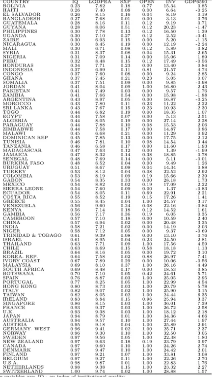
COUNTRY IQ LGDPEA SXP OPEN INV GDP6590 BOLIVIA 0.23 7.82 0.18 0.77 15.34 0.85 HAITI 0.26 7.40 0.08 0.00 6.64 -0.25 EL SALVADOR 0.26 8.15 0.16 0.04 8.19 0.19 BANGLADESH 0.27 7.68 0.01 0.00 3.13 0.76 GUATEMALA 0.28 8.16 0.11 0.12 9.19 0.71 GUYANA 0.28 8.06 0.51 0.12 20.23 -1.47 PHILIPPINES 0.30 7.78 0.13 0.12 16.50 1.39 UGANDA 0.30 7.10 0.27 0.12 2.52 -0.41 ZAIRE 0.30 6.93 0.15 0.00 5.20 -1.15 NICARAGUA 0.30 8.45 0.19 0.00 12.19 -2.24 MALI 0.30 6.71 0.08 0.12 5.89 0.82 SYRIA 0.31 8.37 0.08 0.04 15.31 2.65 NIGERIA 0.31 7.09 0.14 0.00 15.06 1.89 PERU 0.32 8.48 0.15 0.12 17.49 -0.56 HONDURAS 0.34 7.71 0.23 0.00 13.40 0.84 INDONESIA 0.37 6.99 0.11 0.81 21.57 4.74 CONGO 0.37 7.60 0.08 0.00 9.24 2.85 GHANA 0.37 7.45 0.21 0.23 5.05 0.07 SOMALIA 0.37 7.51 0.09 0.00 9.85 -0.98 JORDAN 0.41 8.04 0.09 1.00 16.80 2.43 PAKISTAN 0.41 7.49 0.03 0.00 9.57 1.76 ZAMBIA 0.41 7.66 0.54 0.00 15.98 -1.88 ARGENTINA 0.43 8.97 0.05 0.00 16.87 -0.25 MOROCCO 0.43 7.80 0.11 0.23 11.22 2.22 SRI LANKA 0.43 7.67 0.15 0.23 10.93 2.30 TOGO 0.44 6.82 0.19 0.00 18.35 1.07 EGYPT 0.44 7.58 0.07 0.00 5.13 2.51 ALGERIA 0.44 8.05 0.19 0.00 27.14 2.28 PARAGUAY 0.44 7.88 0.10 0.08 15.53 2.06 ZIMBABWE 0.44 7.58 0.17 0.00 14.87 0.86 MALAWI 0.45 6.68 0.21 0.00 11.29 0.92 DOMINICAN REP 0.45 7.85 0.13 0.00 17.75 2.12 TUNISIA 0.46 7.81 0.10 0.08 14.54 3.44 TANZANIA 0.46 6.58 0.17 0.00 11.60 1.93 MADAGASCAR 0.47 7.63 0.12 0.00 1.39 -1.99 JAMAICA 0.47 8.32 0.14 0.38 18.85 0.78 SENEGAL 0.48 7.69 0.14 0.00 5.11 -0.01 BURKINA FASO 0.48 6.52 0.04 0.00 9.49 1.26 URUGUAY 0.51 8.67 0.09 0.04 14.34 0.88 TURKEY 0.53 8.12 0.04 0.08 22.52 2.92 COLOMBIA 0.53 8.19 0.09 0.19 15.66 2.39 GABON 0.54 8.35 0.33 0.00 28.18 1.73 MEXICO 0.54 8.82 0.02 0.19 17.09 2.22 SIERRA LEONE 0.54 7.60 0.09 0.00 1.37 -0.83 ECUADOR 0.54 8.05 0.11 0.69 22.91 2.21 COSTA RICA 0.55 8.52 0.19 0.15 17.26 1.41 GREECE 0.55 8.45 0.04 1.00 24.57 3.17 VENEZUELA 0.56 9.60 0.24 0.08 22.16 -0.84 KENYA 0.56 7.14 0.18 0.12 14.52 1.61 GAMBIA 0.56 7.17 0.36 0.19 6.05 0.35 CAMEROON 0.57 7.10 0.18 0.00 10.59 2.40 CHINA 0.57 6.94 0.02 0.00 20.48 3.35 INDIA 0.58 7.21 0.02 0.00 14.19 2.03 NIGER 0.58 7.12 0.05 0.00 9.37 -0.69
TRINIDAD & TOBAGO 0.61 9.39 0.08 0.00 13.10 0.76
ISRAEL 0.61 8.95 0.04 0.23 24.50 2.81 THAILAND 0.63 7.71 0.09 1.00 17.56 4.59 CHILE 0.63 8.69 0.15 0.58 18.18 1.13 BRAZIL 0.64 8.16 0.05 0.00 19.72 3.10 KOREA. REP. 0.64 7.58 0.02 0.88 26.97 7.41 IVORY COAST 0.67 7.89 0.29 0.00 10.06 -0.56 MALAYSIA 0.69 8.10 0.37 1.00 26.16 4.49 SOUTH AFRICA 0.69 8.48 0.17 0.00 18.53 0.85 BOTSWANA 0.70 7.10 0.05 0.42 24.61 5.71 SPAIN 0.76 8.87 0.03 1.00 25.05 2.95 PORTUGAL 0.77 8.25 0.05 1.00 22.99 4.54 HONG KONG 0.80 8.73 0.03 1.00 20.79 5.78 ITALY 0.82 9.07 0.02 1.00 25.90 3.15 TAIWAN 0.82 8.05 0.02 1.00 24.44 6.35 IRELAND 0.83 8.84 0.15 0.96 25.94 3.37 SINGAPORE 0.86 8.15 0.03 1.00 36.01 7.39 FRANCE 0.93 9.37 0.03 1.00 26.72 2.58 U.K. 0.93 9.38 0.03 1.00 18.12 2.18 JAPAN 0.94 8.79 0.01 1.00 34.36 4.66 AUSTRALIA 0.94 9.57 0.10 1.00 27.44 1.97 AUSTRIA 0.95 9.18 0.04 1.00 25.89 2.91 GERMANY. WEST 0.96 9.41 0.02 1.00 25.71 2.37 NORWAY 0.96 9.30 0.10 1.00 32.50 3.05 SWEDEN 0.97 9.56 0.05 1.00 22.38 1.80 NEW ZEALAND 0.97 9.63 0.18 0.19 23.79 0.97 CANADA 0.97 9.60 0.10 1.00 24.26 2.74 DENMARK 0.97 9.47 0.10 1.00 24.42 2.01 FINLAND 0.97 9.21 0.07 1.00 33.81 3.08 BELGIUM 0.97 9.27 0.11 1.00 22.26 2.70 U.S.A. 0.98 9.87 0.01 1.00 22.83 1.76 NETHERLANDS 0.98 9.38 0.15 1.00 23.32 2.27 SWITZERLAND 1.00 9.74 0.02 1.00 28.88 1.57
The variables are: IQ - an index of institutional quality,
LGDPEA - the log of GDP per head of the economically active population in 1965,
SXP - the share of primary exports in GNP in 1970, OPEN - an index of a country’s openness INV - the average ratio of real gross domestic investments over GDP
GDP6590– average growth rate of real GDP per capita between 1965 and 1990 For more details see Sachs and Warner (1997a)