Measuring the Fiscal Stance

Discussion Papers in Economics

No. 2000/62

Dynamics of Output Growth, Consumption and Physical Capital

in Two-Sector Models of Endogenous Growth

by

Department of Economics and Related Studies University of York

Heslington

No. 2007/14

Measuring the Fiscal Stance

By

Measuring the Fiscal Stance

Vito Polito

and

Mike Wickens

University of York

Revised July 2006

Abstract

In this paper we propose an index of thefiscal stance suitable for practical use in short-term policy

making. The index is based on a comparison of a target level of the debt-GDP ratio for a given finite

horizon with a forecast of the debt-GDP ratio based on a VAR formed from the government budget

con-straint. This approach to measuring thefiscal stance is different from the literature onfiscal sustainability.

We emphasise the importance of having a forward-looking measure of thefiscal stance for the immediate

future rather than a test forfiscal sustainability that is backward-looking, or based just on past behaviour

which may not be closely related to the current fiscal position. We use our methodology to construct a

time series of the indices of the fiscal stances of the US, the UK and Germany over the last 25 or more

years. We find that both the US and UK fiscal stances have deteriorated considerably since 2000 and

Germany’s has been steadily deteriorating since unification in 1989, and worsened again on joining EMU.

Keywords: Budget deficits, government debt,fiscal sustainability, VAR analysis.

1

Introduction

Recent concerns in 2004 and 2005 about thefiscal stances of the US, France and Germany and of

possible reforms to the EU’s Stability and Growth Pact (largely due to the errant fiscal positions

of France and Germany) have renewed interest in the issue of how to measure the fiscal stance.

In this paper we propose an index of the fiscal stance suitable for practical use in short-term

policy making. We take a very different approach from the literature onfiscal sustainability even

though, like this literature, it is based on the government inter-temporal budegt constraint. We

emphasise the importance of having a forward-looking measure of thefiscal stance that focuses on

the implications of the current fiscal stance for the immediate future. We argue against focusing

on formal tests of the stationarity of debts and deficits as they are backward-looking and not

necessarily a good guide to the current stance offiscal policy.

The index is based on a comparison of a target level of the debt-GDP ratio for a givenfinite

horizon with a forecast of the debt-GDP ratio based on a VAR formed from the government

budget constraint. By using a VAR forecasting model we avoid basing the index on a particular

theoretical model of the economy, and the index is simple to compute and readily automated.

We use our methodology to examine thefiscal stances of the US, the UK and Germany over

the last 25 or more years. We find that both the US and UK fiscal stances have deteriorated

considerably since 2000 and Germany’s has been steadily deteriorating since unification in 1989

and worsened again on joining EMU.

The emphasis on thefiscal stance, as opposed tofiscal sustainability, is a key feature of this

paper. Determining whether the current fiscal stance is sustainable has proved difficult and

con-troversial, and has limited applicability in evaluating fiscal policy in the short run. Typically,

tests for fiscal sustainability focus on the dynamic properties of past debts and deficits and

as-sume that these processes will continue into the infinite future with a view to establishing whether

oblig-ations. There are obvious problems with this approach. First, a failure to satisfy a test for fiscal

sustainability does not necessarily have any implications for the current fiscal stance. A

govern-ment could argue thatfiscal sustainability can be achieved by changing futurefiscal policy so that

sufficient surpluses would be generated. Or, it may be that rejection offiscal sustainability was

due to past fiscal policy and that subsequent changes had removed the problem. In both cases,

the time series properties of past debts and deficits would no longer be relevant for current policy.

Second, a failure to satisfy a test forfiscal sustainability has little immediate relevance iffinancial

markets are still willing to hold government debt, perhaps in the belief that governments will make

the appropriate changes tofiscal policy in the future. Third, a test statistic is not a user-friendly

way of representing fiscal policy. Something more transparent is required such as an index

se-ries that can capture changes in the fiscal stance over time. Fourth, in the related literature on

inter-temporal current account sustainability, the outcome of the test for sustainability depends

on whether consumption is modelled correctly. We seek a measure of the fiscal stance based on

the government constraint that is theory free.

Although the outcome of tests for fiscal sustainability have not played much of a role in

discussions on fiscal policy, a measure of the current fiscal stance would still be helpful. Such

a measure should be easy to represent and compute and not depend on a particular theoretical

model of the economy. Governments need to know the likely consequences of their current fiscal

stance for their debt obligations and the costs of borrowing and of servicing the debt. Markets

need to know the risks associated with the fiscal stance in order to price government debt. The

Maastricht Treaty was an attempt to ensure thatfiscal policy was set appropriately in the run-up

to EMU so that the temptation to inflate away debts was avoided. Its successor, the Stability

and Growth Pact, seeks to avoidfiscal spillovers from one country to another which might affect

monetary policy or euro-debt obligations. It is increasingly recognised, however, that such fiscal

rules are neither necessary nor sufficient. Whatever thefiscal framework, a crucial ingredient is

The index we propose is concerned with forecasting whether the debt-GDP ratio is likely to

exceed or fall below a pre-specified target over a pre-specified time horizon. Given the time horizon

and the target level of the debt-GDP ratio at the end of that horizon, the index is based on a

comparison of the desired change in the debt-GDP ratio and a forecast of the present value of the

current level of the debt-GDP ratio over the horizon derived from a simple VAR forecasting model

of the economy. If the index exceeds unity then the currentfiscal stance is said to be inconsistent

with the debt objective over the horizon in the sense that debt is forecast to rise above target; if

the index is less than unity then the fiscal stance is said to be consistent with the debt objective.

The choice of a VAR model is to avoid taking a particular view of the economy and to permit

the method to be easily automated. The VAR is based on a log-linear approximation to the

government’s inter-temporal budget constraint in order that interest rates, inflation and growth

are allowed to be time varying. This approach is in contrast to much of the literature on fiscal

sustainability where interest rates, inflation and growth are held constant over the forecast horizon

in order to eliminate the non-linearities that their time variation would introduce into the

inter-temporal budget constraint.

The paper is set out as follows. In Section 2 we examine a number of different ways of writing

the government budget constraint and establish our notation. In Section 3 we present an analysis

offiscal sustainability with a view to showing its limitations in providing a useful measure of the

currentfiscal stance. We provide an intuitive rationale for the various tests forfiscal sustainability

that have been proposed in the literature and discuss the technical problems in implementing

these tests. We then show how, by using a log-linear approximation to the government budget

constraint, fiscal sustainability can be tested in a way that permits the discount rate to be

time-varying and enables linear methods of analysis to be used once more. We also comment on the

implications of this analysis of fiscal sustainability for the debt and deficit limits of the EU’s

Stability and Growth Pact. We derive our proposedfiscal index in Section 4 and show how it can

Germany over the period from the 1970’s to 2005. Ourfindings are summarized in Section 6.

2

The government budget constraint

We begin by considering the nominal government budget constraint (GBC), the sustainability of

fiscal policy and the implications of variousfiscal rules, such as the EU’s Stability and Growth

Pact.1 _{The nominal GBC can be written}

Ptgt+ (1 +Rt)Bt−1=Bt+∆Mt+PtTt (1)

where gt is real government expenditure including real transfers to households, Tt is total real

taxes and Mt is the stock of outside nominal, non-interest bearing money in circulation that is

supplied by the government (the central bank) at the start of period t,Btis the nominal value of

government bonds issued at the end of period t, Rt is the average interest rate on bonds issued

at the end of period t₋1and RtBt−1 is total interest payments made in period t.2 Thus the

left-hand side of equation (1) is total nominal expenditures in period tand the right-hand side is

total revenues plus additions to government current financial resources.

The equivalent real GBC can be derived from the nominal GBC by dividing through the

nominal GBC by the general price levelPt. This gives

gt+ (1 +Rt) Pt−1 Pt Bt−1 Pt−1 =Tt+ Bt Pt +Mt Pt − Pt−1 Pt Mt−1 Pt−1

1 _{There is a substantial literature on these issues. Most of it goes back some way in time. See, for example,}

Hamilton and Flavin (1986), Trehan and Walsh (1988, 1991), Kremers (1989), Wilcox (1989), Blanchard, Chouraqui, Hagemann and Sartor (1990), Bohn (1991, 1992, 1995, 1998, 2005), Hakkio and Rush (1991), Buiter, Corsetti and Roubini (1993), Ahmed and Rogers (1995) and Wickens and Uctum (2000). There is also a related literature on current account sustainability, see Sheffrin and Woo (1990) and Bergin and Sheffrin (2000) for a discussion of the inter-temporal approach to the current account and Wickens and Uctum (1993) for analaysis of the sustainability of a country’s net asset position.

2 _{In practice governments issue bonds at a discount and redeem them at par. Thus if all bonds were for one}

period, thenBt=PtBBGt whereBtGis the number of bonds issued in periodteach with pricePtB= 1 1+Rt+1 and

BG

or

gt+ (1 +rt)bt−1=Tt+bt+mt−

1 1 +πt

mt−1 (2)

whereπt= _P∆_tP₋t₁ is the rate of inflation,btis the real stock of government debt,mtis the real stock

of money andrtis the real rate of interest which, in view of our dating convention, is defined by

1 +rt=

1 +Rt

1 +πt

Thus, approximately, rt'Rt−πt.

The GBC can also be expressed in terms of proportions of nominal or real GDP by dividing

through the nominal GBC by Ptyt, nominal GDP, whereytis real GDP. We obtain

gt yt + 1 +Rt (1 +πt)(1 +γt) bt−1 yt−1 = Tt yt +bt yt +mt yt − 1 (1 +πt)(1 +γt) mt−1 yt−1 (3)

where γ_tis the rate of growth of GDP and Tt

yt is the average tax rate.

The total nominal government deficit (or public sector borrowing requirement, PSBR) is

de-fined as

PtDt=Ptgt+RtBt−1−PtTt−∆Mt

Hence Dt

yt, the real government deficit as a proportion of GDP, is

Dt yt = gt yt + Rt (1 +πt)(1 +γt) bt−1 yt−1 − Tt yt − mt yt + 1 (1 +πt)(1 +γt) mt−1 yt−1 = bt yt − 1 (1 +πt)(1 +γt) bt−1 yt−1

The right-hand side shows the net borrowing required to fund the deficit expressed as a proportion

of GDP.

We also define the nominal primary deficitPtdt(the total deficit less debt interest payments)

as

Ptdt=PtDt−RtBt−1

which implies that

dt yt = Dt yt − Rt (1 +πt)(1 +γt) bt−1 yt−1

Hence the ratio of the primary deficit to GDP is dt yt = gt yt − Tt yt − mt yt + 1 (1 +πt)(1 +γt) mt−1 yt−1 = bt yt − 1 +Rt (1 +πt)(1 +γt) bt−1 yt−1 (4)

This is a non-linear difference equation in bt

yt. If we define

1 +ρ_t= 1 +Rt (1 +πt)(1 +γt)

where approximately,ρ_t=Rt−πt−γt=rt−γt, is the real interest rate adjusted for economic

growth, then equation (4) can be written as

bt yt = (1 +ρ_t)bt−1 yt−1 +dt yt (5)

This is the key equation for determining the sustainability of fiscal policy. The stability of the

equation depends on the sign ofρ_t.

We note that the evolution of bt

yt can also be written in terms of the total deficit since

bt yt = 1 (1 +πt)(1 +γt) bt−1 yt−1 +Dt yt (6)

For positive inflation and growth this is a stable difference equation

3

Fiscal sustainability

Fiscal sustainability concerns the evolution of bt

yt and whether it remains finite or explodes. In

this and subsequent sections we adopt the common terminology that the fiscal stance is said to

be sustainable if bt

yt is finite - and if financial markets are willing to hold the level of debt that

emerges. Before describing our proposed new procedure for determining whether thefiscal stance

is consistent with given debt objectives, we review the principal methods in the literature for

testing what is referred to as fiscal sustainability. All take equation (5) as their starting point.

rate ρ_t (and hence Rt,πt and γt) is assumed to be constant and where it is allowed to be time

varying.3

3.1

Constant discount rate

If ρ_t is assumed to be constant then, from equation (5), bt

yt evolves according to the difference

equation bt yt = (1 +ρ)bt−1 yt−1 +dt yt (7)

where 1 +ρ = ₍₁₊1+_π)(1+R _γ) or, approximately, ρ = R₋π₋γ. The solution for bt

yt depends on

whether the equation (7) is stable or unstable. We consider both cases.

Case1: ρ <0(stable case)

In this case ₍₁₊1+_π)(1+R _γ) < 1 and equation (7) is a stable difference equation, and hence can

be solved backwards by successive substitution. The expected value of the debt-GDP ratio in n

period’s time conditional on information at timet is

Et( bt+n yt+n ) = (1 +ρ)n bt yt + n−1 X s=0 (1 +ρ)n−sEt( dt+s yt+s ) (8)

Taking the limit asn_{→ ∞}gives

lim

n→∞(1 +ρ)

nbt

yt

= 0 (9)

implying that the current level of debt has no bearing on debt in the infinite future.

If (9) holds then we obtain

lim n→∞Et( bt+n yt+n ) = lim n→∞ n X s=1 (1 +ρ)n−sEt( dt+s yt+s ) (10)

The evolution of the debt-GDP ratio depends on that ofdt

yt. Suppose that

dt

yt may be stochastic

but is expected to grow at the rateλsuch that

Et( dt+s yt+s ) = (1 +λ)sdt yt (11)

3_{Ahmed and Rogers (1995) and Bohn (1995, 2005) argue that the appropriate discount rate to use for discounting}

future primary surpluses is the inter-temporal marginal rate of substitution and not the real interest rate. In a complete markets full general equilibrium model this would be the real rate of return used here.

It follows that lim n→∞Et( bt+n yt+n ) = lim n→∞ n X s=1 (1 +ρ)n−s(1 +λ)sdt yt = lim n→∞(1 +λ) µ (1 +λ)n_{−(1 +ρ)}n λ₋ρ ¶ dt yt = ₋1 ρ dt yt if λ= 0 (12)

If ρ, λ <0thenlimn→∞Et(_yb_tt+₊n_n) = 0. If λ > 0then it will explode. Thus, the debt-GDP ratio

will remainfinite and positive if (₋dt

yt), the ratio of the primary surplus to GDP, does not explode.

We note that ifλ <0then dt

yt is a stationary I(0) process and the expected, or long-run, value of

the debt-GDP ratio is zero. And ifλ= 0, then dt

yt is a non-stationary I(1) process, and hence

bt

yt

will also be I(1). Moreover, bt

yt and

dt

yt will be cointegrated with cointegrating vector(1,

1

ρ). Fiscal

policy is therefore sustainable provided bt

yt does not grow over time.

Case 2: ρ >0(unstable case)

In this case0< (1+π₁₊)(1+_R γ) <1. Equation (7) is therefore an unstable difference equation and

must be solved forwards, not backwards, as follows:

bt yt = 1 1 +ρEt( bt+1 yt+1 − dt+1 yt+1 ) = (1 +ρ)−nEt( bt+n yt+n )₋ n X s=1 (1 +ρ)−sEt( dt+s yt+s ) (13)

Taking limits asn_{→ ∞}gives the transversality condition lim n→∞(1 +ρ) −n Et( bt+n yt+n ) = 0 (14)

If this holds then

bt yt = ∞ X s=1 (1 +ρ)−sEt(− dt+s yt+s ) (15)

implying that the expected present value of current and future primary surpluses expressed as

a proportion of GDP (the right-hand side of equation (15)) must be sufficient to pay-offcurrent

Suppose once more that dt

yt is expected to evolve according to equation (11) then

bt yt = ∞ X s=1 (1 +ρ)−s(1 +λ)s(−dt yt ) (16) = 1 +λ ρ₋λ( −dt yt ) if ₋1< λ < ρ, ρ >0

Thus, if ₋1< λ < ρ and ρ > 0, the present value of primary surpluses will meet current debt obligations. However, the debt-GDP ratio will grow at the rateλ, the same rate as −dt

yt .

If ₋1< λ <0 then −dt

yt is stationary and

bt

yt will also be stationary and finite. If λ= 0, so

that −dt

yt is I(1), then we obtain the same condition as equation (12), namely,

bt yt = 1 ρ( −dt yt ) (17) implying that bt

yt will be I(1) and will be cointegrated with

−dt

yt with cointegrating vector (1,−

1

ρ).

These results provide an insight into the rationale behind a number of well-known empirical

tests for fiscal sustainability. The test of Hamilton and Flavin (1986) is based on the following

version of equation (13) bt yt =A0(1 +ρ)−t− ∞ X s=1 (1 +ρ)−sEt( dt+s yt+s )

except that real debt and the real primary deficit is used rather thanbt

yt and

dt

yt. The transversality

condition holds on the null hypothesis that .A0= 0.

Trehan and Walsh (1988) propose a cointegration test forfiscal sustainability. They measure

debt and the primary deficit in real terms rather than as proportions of GDP, but Hakkio and

Rush (1991) employ the test expressing the variables as proportions of GDP. We have already

seen from equations (12) and (17) that if the variables have unit roots and are cointegrated with

cointegrating vector(ρ,1)thenfiscal policy is sustainable. (Or, if the primary deficit is decomposed

into government expenditures and revenues and both are I(1), then the cointegrating vector with

debt must be (ρ,1,₋1).)

Alternatively, if there is a cointegrating relation between debt and the primary deficit given by

dt

yt

+αbt yt

for some αand stationaryut, then from equation (7), (1 +α)bt yt = (1 +ρ)bt−1 yt−1 +ut It follows that bt

yt has a unit root ifα=ρ.

3.2

Time-varying discount rate

In practice,ρ_twill be time-varying, not constant, and so these tests will in general be invalid. If

ρ_t<0then the budget constraint, equation (5), will be stable and the debt-GDP ratio will remain

finite if dt

yt is stationary.

Ifρt>0then we solve the budget constraint forwards to obtain

bt yt =Et[(Πns=1 1 1 +ρ_t+s) bt+n yt+n ]₋Et[ n X s=1 (Πs_i=1 1 1 +ρ_t+i) dt+s yt+s ] (18) if δt,s=Πsi=1 1 1 +ρ_t+i ≤1 f or all s≥1

Hence fiscal solvency depends on the transversality condition

lim n→∞Et[(Π n s=1 1 1 +ρ_t+s) bt+n yt+n ] = 0 (19)

If this holds then

bt yt =Et[ ∞ X s=1 (Πs_i=1 1 1 +ρ_t+i)( −dt+s yt+s )] (20)

Like equation (15), equation (20) says that the present value of current and future primary

sur-pluses must be sufficient to offset current debt liabilities. The difference is that the discount rate

is compounded from time-varying rates.

In order to analyse sustainability we define the variables

xt = δt,n bt yt zt = δt,n dt yt

We may now write equation (5) as

∆xt=zt

Fiscal sustainability now requires the transversality condition

lim

n→∞Et(xt+n) = 0 and implies that

xt=− lim n→∞Et[ n X s=1 zt+s]

Wilcox (1989) shows thatfiscal sustainability is satisfied ifxtis a zero-mean stationary process.

Uctum and Wickens (2000) prove a more general result that does not requirextto be stationary.

They show that fiscal sustainability is satisfied if zt is a zero-mean stationary process when it

follows that xt will be an I(1) process.

3.3

Fiscal sustainability and the total de

fi

cit

Another approach tofiscal sustainability is to focus on the relation between the debt and the total

deficit, rather than the primary deficit. This is given by equation (6) which is a stable difference

equation ifπt+γt, the rate of growth of nominal GDP, is positive. If, in addition, Dytt is stationary

then bt

yt will be stationary and hence remainfinite.

Trehan and Walsh (1991) therefore argue thatfiscal policy is sustainable with a variable

dis-count rate if the total deficit is stationary. We also note from previous results that the stationarity

of Dt

yt is a consequence of the cointegration of

bt

yt and

dt

yt, andvice-versa.

3.4

Stability and Growth Pact (SGP)

The SGP was based on the original Maastricht conditions that bt

yt must be less than 0.6and

Dt

yt

must be less than 0.03. For given values of bt

yt and Dt yt bounded above by bt yt and D y and for a

constant nominal growth rate the long-run solution to equation (6) is b y = (1 +π)(1 +γ) (1 +π)(1 +γ)₋1 D y ' 1 π+γ D y

It follows that nominal growth must satisfy

π+γ_'

D y b y

Hence, given the limits on debt and deficits specified under the SGP, the nominal rate of growth

must not be less than 0₀._.03_{6 ≡}5%. If nominal growth were less than this then debt would rise above 60% even if the deficit limit were satisfied. Although the debt-GDP ratio would exceed the SGP

limit, it would still satisfy the condition for fiscal sustainability.

Now suppose that the deficit exceeds the3%limit. Whether or not the debt-GDP ratio exceeds

60%depends on the rate of nominal growth. The higher the rate of nominal growth, the less likely

is the debt-GDP ratio to exceeds its limit. Once again, this does not affectfiscal sustainability.

It follows that the SGP is neither necessary nor sufficient forfiscal sustainability in the long

run. This is becausefiscal sustainability may be satisfied even if the SGP limits are breeched and

because it is also necessary that the rate of nominal growth is appropriate.

3.5

A log-linear approach to

fi

scal sustainability

To complete our discussion of fiscal sustainability, we propose an alternative way to deal with a

time-varying discount rate which we make use of later. This is to use a log-linear approximation

to the government budget constraint taken about the steady-state solution (assuming it exists).

As the primary deficit can take negative values, it is necessary to write the GBC in terms of total

expenditures gt and total revenuesvt both of which are strictly positive. We therefore re-write

the GBC, equation (3), as bt yt = gt yt− vt yt + (1 +ρ_t)bt−1 yt−1

where vt yt =Tt yt +mt yt − 1 (1 +πt)(1 +γt) mt−1 yt−1

Next we approximate the GBC about the steady-state solution in which we assume that all

variables are constant. The steady-state solution to the GBC is

ρb y =− g y + v y

The GBC may be re-written as

f(xt) = exp [ln bt yt ]₋exp [lngt yt ]+ exp [lnvt yt ]₋exp [ln (1 +ρ_t) + lnbt−1 yt−1 ] = 0

Noting that a first-order Taylor series approximation toh(xt) = exp[lnxt]aboutlnxis

h(xt)'x[1 + (lnxt−lnx)]

a log-linear approximation to the GBC about the steady-state is given by

ln bt yt ' c+g b ln gt yt− v b ln vt yt + (1 +ρ) ln(1 +ρ_t) + (1 +ρ)lnbt−1 yt−1 (21) c = ₋ρlnb y − g bln g y+ v bln v y −(1 +ρ) ln(1 +ρ)

Asln(1 +ρt)'ρt, in effect, the discount rate is an additional variable in the equation.

Using equation (21),fiscal sustainability may be analysed with a linear model even though the

discount rate is time-varying. The stability of the log-linearized GBC depends on the sign of ρ.

Assuming thatρ >0, we solve the equation forwards to obtain

lnbt yt = (1 +ρ)−nEt(ln bt+n yt+n )₋ n X s=1 (1 +ρ)−sEt(kt+s) (22) kt = c+ g bln gt yt− v bln vt yt + (1 +ρ) ln(1 +ρ_t) (23)

wherektis, in effect, the logarithmic equivalent of the primary deficit. The transversality condition

is therefore lim n→∞(1 +ρ) −n Et(ln bt+n yt+n ) = 0 (24)

which implies that lnbt yt =₋ ∞ X s=1 (1 +ρ)−sEt(kt+s) (25)

If kt is stationary then ln_yb_tt, and hence b_yt_t, remains stationary and finite. This may occur

due to the individual terms of kt being stationary, or due to some terms being I(1) but being

cointegrated. From equation (21), the cointegrating equation is

ln bt yt '− c ρ− g ρbln gt yt + v ρbln vt yt − 1 +ρ ρ ln(1 +ρt)

4

An index of the

fi

scal stance

4.1

An assessment of the tests for

fi

scal sustainability

All of these tests of fiscal sustainability, including the new log-linear test that we propose, are of

limited practicality. The main problem is that the tests are based on the past behaviour of debts

and deficits whereas the sustainability of currentfiscal stance is related to their future behaviour.

The test outcome could be dominated by an influential, but anomalous, period in the distant

past yet the current fiscal stance may still be sustainable. Even if the currentfiscal stance is not

sustainable, governments could claim that a policy change planned for the future would make it

sustainable. As a result, the tests provide an ineffective constraint onfiscal policy, especially in

the near future.

This suggests that we need a more forward-looking approach that focuses on the short-term

implications of the currentfiscal stance. As thefiscal position varies over time, it would be helpful

to have a measure that reflects this and enables historical comparisons to be made. We therefore

propose constructing an index number series of the current fiscal stance.

The index is based on the inter-temporal government budget constraint. The index measures

the ratio of the desired change in the discounted debt-GDP ratio over a given time horizon relative

a particular number such as the 60% SGP limit, a percentage reduction or the maintenance of the

current level of debt.

The forecast change in the debt-GDP ratio is, in effect, the present value of current and future

primary surpluses. Future primary surpluses and discount rates are forecast using a VAR based

on the variables in the governmnent budget constraint. Any other forecasting model could be

used instead, including a structural model of the whole economy. The reasons for choosing a such

a VAR are its simplicity and its ease of replication and automation for any economy. We also

wish to try to avoid taking a particular view on macroeconomic theory and on the structural of

the economy. Since time variation in the future discount rate may be of importance, we base the

VAR on our log-linear approximation to the government budegt constraint.

The use of an index of sustainability was initially proposed by Blanchard, Chouraqui,

Hage-mann, and Sartor (1990) and Buiter, Corsetti and Roubini (1993). Their indices are based on a

comparison of the current debt-GDP ratio and that n periods ahead with givenfixed values of

the deficit and discount rate. By allowing the deficit and discount rate to be time-varying and

endogenous, and the target level of the debt-GDP ratio to be a choice variable, we generalize these

indices.

4.2

Constructing the index

The basis of our proposed index is the inter-temporal log-linearized budget constraint equation

(22). This can be re-written as

(1 +ρ)−nEt(ln bt+n yt+n )₋lnbt yt = n X s=1 (1 +ρ)−sEt(kt+s)

If we replaceEt[ln_ybt_t+₊n_n]by the targetln(b_yt_t+₊n_n)∗ we obtain

(1 +ρ)−nln(bt+n yt+n )∗₋lnbt yt = n X s=1 (1 +ρ)−sEt(kt+s) (26)

The left-hand side of equation (26) can be interpreted as the desired change in discounted debt

value of the primary surpluses required to achieve this desired change in discounted debt. We

replaceEt(kt+s)by forecasts of the future values ofktbased on the information available at time

t, including the currentfiscal stance.

A measure of whether the currentfiscal stance is likely to achieve the debt objective is obtained

by comparing the two sides of equation (26). If, for example, the aim is to decrease discounted

debt then the left-hand side will be negative and the right-hand side gives the present value of the

primary surplus required to achieve this reduction in debt. We therefore base our measure of the

consistency of the current fiscal stance with then₋period debt objective on the gap between the objective and the forecast outcome:

F S(t, n) = [(1 +ρ)−nln(bt+n yt+n )∗₋lnbt yt ]₋ n X s=1 (1 +ρ)−sEt(kt+s)R0 Our index is F SI(t, n) = exp[F S(t, n)] = Kt,n bt/yt lnKt,n = (1 +ρ)−nln( bt+n yt+n )∗₋ n X s=1 (1 +ρ)−sEt(kt+s) kt = c+ g bln gt yt − v b ln vt yt + (1 +ρ) ln(1 +ρt) c = ₋ρlnb y − g bln g y+ v bln v y −(1 +ρ) ln(1 +ρ)

As n_{→ ∞}thefirst term in lnKt,n tends to zero and the index can be interpreted as comparing

the the existing level of the debt-GDP ratio with the resources to pay it off.

The index may be interpreted as follows:

(i) ifF SI(t, n) = 1the debt-GDP ratio in periodt+nis forecast to be on target

(ii) ifF SI(t, n)>1the debt-GDP ratio is forecast to be below target

(iii) ifF SI(t, n)<1the debt-GDP ratio is forecast to be above target.

Only in case (iii) is the forecasted present value of the primary surplus insufficient to achieve

sustainable.

In practice, the special case considered by Buiter and Blanchard of maintaining a constant

debt-GDP ratio over the planning horizon will often be of most interest. In this case

F S(t, n) = [(1 +ρ)−n₋1] lnbt yt− n X s=1 (1 +ρ)−sEt(kt+s)R0

The index then becomes

F SI(t, n) = exp[F S(t, n)] = Kt,n bt/yt (27) lnKt,n = (1 +ρ)−nln bt yt − n X s=1 (1 +ρ)−sEt(kt+s)

Since in this case

lnbt yt = (1 +ρ)−nlnbt yt− n X s=1 (1 +ρ)−sEt(kt+s) = ₋ 1 1₋(1 +ρ)−n n X s=1 (1 +ρ)−sEt(kt+s) ' −_nρ1 n X s=1 (1 +ρ)−sEt(kt+s)

the index could also be calculated as

F SI(t, n) = K ∗ t,n bt/yt (28) lnK_t,n∗ = ₋ 1 1₋(1 +ρ)−n n X s=1 (1 +ρ)−sEt(kt+s)

where the numerator of the index is now proportional to the present value of primary surpluses.

We consider this case in our empirical examples below.

4.3

Forecasting the

fi

scal variables

In order to compute the index we require forecasts of the variables of the following vector zt

zt= µ lnbt yt , lngt yt , lnvt yt , ln(1 +ρ_t), ln(1 +γ_t), ln(1 +πt) ¶0

For the reasons given above, we use of a VAR(p) to obtain these forecasts. This is a simple

forecasting scheme that is easily implemented and is theory free. We denote the VAR by

zt=A0+

p

X

i=1

Aizt−i+et, (29)

where et∼i.i.d.[0,Σ]. The vector of variables ztmay be I(0) or I(1). For forecasting purposes it

is unnecessary to take account any non-stationarity or cointegration among the variables. Equally,

if cointegration exists, a cointegrated VAR could be estimated instead of a levels VAR and the

cointegrated VAR could then be written in levels to obtain equation (29). We also note that to

improve the forecasts, zt could contain additional variables to those that appear in the budget

constraint.

n₋period ahead forecasts may be obtained using the companion form Zt=B0+BZt−1+ut. where Z0 t=[z0t,z0t−1, ...,zt−p+1], u0t=[e0t,0, ...,0], B00= [A00,0, ...,0]and B= ⎡ ⎢ ⎢ ⎢ ⎢ ⎢ ⎢ ⎢ ⎢ ⎢ ⎢ ⎢ ⎢ ⎢ ⎢ ⎣ A1 A2 . . Ap−1 0 I 0 . . 0 . I 0 . . . . . . . . 0 I 0 ⎤ ⎥ ⎥ ⎥ ⎥ ⎥ ⎥ ⎥ ⎥ ⎥ ⎥ ⎥ ⎥ ⎥ ⎥ ⎦

The forecast ofZt+n is therefore

Et[Zt+s] =

s−1

X

i=0

BiB0+BsZt

Defining the selection matrixS=[I,0,0, ..,0]such that

zt=SZt

and expressingktas the following linear function of zt

we obtain F S(t, n) = lnK_t,n∗ ₋lnbt yt = ₋ 1 1₋(1 +ρ)−n n X s=1 {(1 +ρ)−s[a+β0S( s−1 X i=0 BiB0+BsZt)]}−ln bt yt

As the last termlnbt

yt is another linear function ofZt, F S(t, n)could also be written as

F S(t, n) =an+b0nZt

where an is a scalar dependent on the time horizon and bn is a vector. This emphasises that

F S(t, n)is based on information available at time t and, in particular, the currentfiscal stance.

Increasing the forecast horizon altersan andbn but notZt.

To implement this in practice it will be necessary to deriveanandbnfrom the VAR estimates.

The choice ofρandcmay be based, for example, on the average values in the sample, their average

values over the forecast period or their timetvalues. A time series forF S(t, n)may be calculated

from the sample either using all of the sample observations to estimate the VAR, or recursively

using only observations up to periodt.

5

Indices of the

fi

scal stances of the US, the UK and

Ger-many

We now construct a time series of the index of thefiscal stance for the US, the UK and Germany.

For the US we consider three horizons: one-year, two-years andfive-years ahead. For the UK and

Germany we use just a one-year horizon. We assume that the aim in each period is to maintain

the current level of the debt-GDP ratio. Hence, we use the version of the index given by equation

(28). The data are quarterly from 1960-2005 for the US and from 1970-2005 for the UK, but are

annual from 1977-2005 for Germany. The data sources and the construction of the variables are

described in the Appendix. There are minor differences in definitions for the different countries.

Maastricht definition of debt but, given the definitions of the other variables, is consistent with

the government budget constraint.

In calculating the present values we require values for v_b, g_b and ρ. We estimate b, g and ρ

using their sample averages. Table 1 gives the average values for Germany, the UK and the US.

Table 1

b g v ρ

Germany 0.290 0.447 0.459 0.041 United Kingdom 0.352 0.405 0.435 0.086 United States 0.423 0.308 0.331 0.054

Note: b, gandρare sample averages,v is constructed from the steady-state equationv=g+ρb

5.1

The United states

Figure 1 gives a plot of eight key variables for the US: bt

yt, gt yt, vt yt, gt−vt yt , Rt, πt, γt, ρt. Thefirst four

variables are expressed as percentages of GDP and the last four are annualised percentages.

1960 1970 1980 1990 2000 30 40 50 60 _b/y 1960 1970 1980 1990 2000 27.5 30.0 32.5 g/y 1960 1970 1980 1990 2000 27.5 30.0 32.5 35.0 v/y 1960 1970 1980 1990 2000 0 5 (g−v)/y 1960 1970 1980 1990 2000 0 5 10 pi 1960 1970 1980 1990 2000 5.0 7.5 R 1960 1970 1980 1990 2000 −5 0 5 rho 1960 1970 1980 1990 2000 0.0 2.5 5.0 _{GDP growth} Figure 1: US data

In Table 1 we report Augmented Dickey-Fuller tests for these variables using up to6lags. We

Table 1

Augmented Dickey-Fuller tests

D-Lag Variable lnb y ln g y ln v y ln (1 +R) ln (1 +pi) ρ ∆lnyt 6 -1.280 -2.305 -2.127 -1.656 -1.984 -1.515 -5.347** 5 -1.734 -2.341 -2.089 -1.749 -2.031 -1.633 -5.415** 4 -2.156 -2.462 -2.076 -1.750 -1.927 -1.774 -5.947** 3 -1.197 -2.836 -2.062 -1.496 -1.704 -1.638 -5.481** 2 -0.7304 -2.511 -2.102 -1.324 -1.896 -2.082 -6.262** 1 -0.8553 -1.996 -1.952 -1.312 -2.375 -2.628 -6.882** 0 -0.4945 -1.824 -2.316 -1.270 -3.098* -3.825** -9.950**

Note: * denotes significance at the5%level and ** denotes significance at the10% level.

As we are using the VAR only for forecasting we estimate a VAR in levels of the variables and

ignore any possible cointegration arising from the variables that have unit roots. For space reasons

we do not report the VAR estimates, but we note that a lag of 6produces serially uncorrelated

residuals.

We examine fiscal sustainability based a constant target debt-GDP ratio for three horizons:

one-year, two-years and five-years ahead. For each horizon we present fourfigures. Figures 2.n

are plots of F SI(n), the index of thefiscal stance. We recall that F SI(n)<1implies that the

debt-GDP ratio is forecast to be above target. The forecasts are based on estimates of the VAR

for the whole sample.

Figures 3-5 give various breakdowns of the index into its component parts. Thus, Figures 3.n

are plots of lnbt

yt and the forecast logarithm of the present value of current and future primary

surpluses,lnKt,n, which we denote in the graph byEP V GBC(n). There are three components to

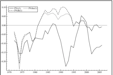
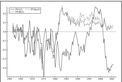
P V s(n)and the term for the discount factor, P V rho(n). These are plotted in Figures 4.n. An

indication of the benefit of using a log-linear model is given by the extent to which P V rho(n)

differs from unity. Finally, in Figures 5.n we plot the two components ofP V s(n). These are the

present value of revenuesP V v(n)and of expendituresP V g(n).

(i) One-year horizon

1960 1965 1970 1975 1980 1985 1990 1995 2000 2005 0.900 0.925 0.950 0.975 1.000 1.025 1.050 1.075 _FSI(1) Figure 2.1: US FSI(1). 1960 1965 1970 1975 1980 1985 1990 1995 2000 2005 30 35 40 45 50 55 b/y EPVGBC(1)

1960 1965 1970 1975 1980 1985 1990 1995 2000 2005 −0.100 −0.075 −0.050 −0.025 0.000 0.025 0.050 PVs(1) PVdb(1) PVrho(1)

Figure 4.1: US PVs(1), PVdb(1) and PVrho(1).

1960 1965 1970 1975 1980 1985 1990 1995 2000 2005 −1.30 −1.25 −1.20 −1.15 −1.10 −1.05 PVv(1) PVg(1) Figure 5.1: US PVv(1) and PVg(1).

1960 1965 1970 1975 1980 1985 1990 1995 2000 2005 0.80 0.85 0.90 0.95 1.00 1.05 1.10 1.15 FSI(2) Figure 2.2: US FSI(2). 1960 1965 1970 1975 1980 1985 1990 1995 2000 2005 25 30 35 40 45 50 55 60 b/y EPVGBC(2)

1960 1965 1970 1975 1980 1985 1990 1995 2000 2005 −0.20 −0.15 −0.10 −0.05 0.00 0.05 0.10 PVs(2) PVdb(2) PVrho(2)

Figure 4.2: US PVs(2), PVdb(2) and PVrho(2).

1960 1965 1970 1975 1980 1985 1990 1995 2000 2005 −2.6 −2.5 −2.4 −2.3 −2.2 −2.1 PVv(2) PVg(2) Figure 5.2: US PVv(2) and PVg(2).

1960 1965 1970 1975 1980 1985 1990 1995 2000 2005 0.7 0.8 0.9 1.0 1.1 1.2 1.3 FSI(5) Figure 2.5: US FSI(5). 1960 1965 1970 1975 1980 1985 1990 1995 2000 2005 20 30 40 50 60 70 b/y EPVGBC(5)

1960 1965 1970 1975 1980 1985 1990 1995 2000 2005 −0.4 −0.3 −0.2 −0.1 0.0 0.1 0.2 PVs(5) PVdb(5) PVrho(5)

Figure 4.5: US PVs(5), PVdb(5) and PVrho(5).

1960 1965 1970 1975 1980 1985 1990 1995 2000 2005 −7.00 −6.75 −6.50 −6.25 −6.00 −5.75 −5.50 −5.25 −5.00 −4.75 PVv(5) PVg(5) Figure 5.5: US PVv(5) and PVg(5).

We observe thatF SI(n), the index of the fiscal stance, exceeds unity for any length of time

only during 1990’s. In the other periods it is either roughly equal to unity (implying that the

fiscal stance is compatible with a non-rising debt-GDP ratio) or less than unity (implying that the

debt-GDP ratio is rising). From 2001 the F SI strongly indicates a rising level of the debt-GDP

ratio at each horizon. The F SI is also less than unity for the period ending in 1989. The start

date of this period depends on the time horizon. For one-year and two-year horizons it is similar,

almost to 1965. Thus the 1990’s marked a period of US fiscal recovery which ended in around

2000.

Decomposing the index into its components, wefind thatF SI <1for the period 1979-1994

when the debt-GDP ratio rose substantially. We alsofind that variations in the present value of

forecast primary surpluses are the main determinant offluctuations in the index. The change in

debt target and the discount factor nearly offset each other. This is because we have assumed a

constant discounted debt target and so the discount factor is the variable causing the change in

discounted debt term to fluctuate.

The present values for expenditures and revenues are similar before 1995 but are different

thereafter. In the period 1995-2001 the present value of revenues exceed those of expenditures

thereby producing afiscal recovery. After 2001 the present value of expenditures exceed those of

revenues. This fiscal deterioration was due to a combination of rising expenditures and sharply

falling revenues. Fluctuations in the discount rate make an additional, but not large, contribution.

To summarize, there is clear evidence of a break in USfiscal policy from 2001 that has resulted

in a rising debt-GDP ratio no matter the horizon over which we look. Thisfiscal stance would be

unsustainable if maintained. The cause is a combination of a rising present value of expenditures

and of sharply falling revenues. There have been previous periods when the fiscal stance also led

to a rising debt-GDP ratio, most notably from 1979-1994. This was not fully corrected until the

period 1995-2000 when the present value of expenditures was reduced and was much lower than

that of revenues.

5.2

The United Kingdom

1970 1980 1990 2000 20 30 40 50 b/y 1970 1980 1990 2000 35 40 45 g/y 1970 1980 1990 2000 40.0 42.5 45.0 v/y 1970 1980 1990 2000 −5 0 5 (g−v)/y 1970 1980 1990 2000 10 20 pi 1970 1980 1990 2000 5 10 15 R 1970 1980 1990 2000 −10 0 10 rho 1970 1980 1990 2000 0.0 2.5 5.0 7.5 Output Growth Figure 6: UK data

Augmented Dickey-Fuller tests are reported in Table 3. We conclude from these results that

lng_y and the real growth rate are stationary variables.

Table 3

Augmented Dickey-Fuller tests (sub-sample 1970-2005)

D-Lag Variable

lnb_y lng_y lnv_y ln (1 +R) ln (1 +pi) ρ ∆lnyt

2 -2.349 -4.184** -2.416 -1.503 -1.267 -1.620 -3.600*

1 -2.432 -3.390* -3.194* -1.362 -1.768 -1.582 -4.595**

0 -1.400 -1.996 -2.250 -0.9936 -1.691 -1.757 -3.981**

Note: * denotes significance at the5%level and ** denotes significance at the10%level.

Based once again on a levels VAR(6), but considering only a one-year horizon, we obtain the

1970 1975 1980 1985 1990 1995 2000 2005 0.825 0.850 0.875 0.900 0.925 0.950 0.975 1.000 1.025 FSI(1) Figure 7: UK FSI(1). 1970 1975 1980 1985 1990 1995 2000 2005 15 20 25 30 35 40 45 50 b/y EPVGBC(1)

1970 1975 1980 1985 1990 1995 2000 2005 −0.20 −0.15 −0.10 −0.05 0.00 0.05 0.10 _PVs(1) PVdb(1) PVrho(1)

Figure 9: UK PVs(1), PVdb(1) and PVrho(1).

1970 1975 1980 1985 1990 1995 2000 2005 −1.05 −1.00 −0.95 −0.90 −0.85 −0.80 PVv(1) PVg(1) Figure 10: UK PVv(1) and PVg(1).

We observe only two brief periods whereF SI >1. These are 1986-1988 and 1997-2000. From

1971-1984 and after 2000F SI <1often by a considerable margin. The period 1984-2005 has four

clear episodes. From 1984-1989 there were falls in the debt-GDP ratio and in both revenues and

expenditures in present value terms resulting in an improving fiscal position. This was a period

where privatization receipts were used to pay offdebt, even though the assets were not included

in our measure of debt, namely, net government liabilities. From 1989-1992, when sterling left

been a contributory factor in the speculation against sterling in 1992. After 1992 the debt-GDP

rose steadily as it did in the US, but expenditures, after continuing to rise, turned down, which

caused an improvement in thefiscal stance. From 1996-2001 there was a marked improvement in

thefiscal position mainly due to rising revenues from the upturn in economic activity. From 2001

thefiscal stance deteriorated again due to expenditures (which started to increase in 1998) rising

much more than revenues. The Chancellor of the Exchequer has said throughout his tenure that

the UK is meeting its fiscal targets, but this evidence indicates that this has not precluded an

obvious decline in the sustainability of the UK’sfiscal stance.

5.3

Germany

The data are annual for the period 1970 to 2005 and are plotted in Figure 11.

1980 1990 2000 20 40 60 _b/y 1980 1990 2000 42.5 45.0 47.5 _g/y 1980 1990 2000 44 46 v/y 1980 1990 2000 −2.5 0.0 2.5 (g−v)/y 1980 1990 2000 0 2 4 pi 1980 1990 2000 20 40 60 R 1980 1990 2000 0 20 40 rho 1980 1990 2000 0 5 10 15 Output Growth

Figure 11: Germany data

The augmented Dickey-Fuller tests reported in Table 4 do not allow us to reject a unit root

for any of the variables

Augmented Dickey-Fuller tests (sub-sample 1976-2005) D-Lag Variable ln_yb lng_y lnv_y ln (1 +R) ln (1 +pi) ρ ∆lnyt 2 -1.315 -2.102 -1.653 -2.016 -1.355 -2.176 -2.515 1 -1.918 -2.080 -1.382 -1.645 -1.635 -2.850 -3.472* 0 -3.582* -2.017 -1.422 -5.303** -2.125 -3.431* -3.680*

Note: * denotes significance at the5%level and ** denotes significance at the10%level.

The results on the index of thefiscal stance for the period from 1977 are reported in Figures

11-15 for a one-year horizon. The reason for starting in 1977 is that prior to this the debt-GDP

ratio was negative.

1980 1985 1990 1995 2000 2005 0.90 0.95 1.00 1.05 1.10 1.15 FSI(1)

1980 1985 1990 1995 2000 2005 10 20 30 40 50 60 b/y EPVGBC(1)

Figure 13: Germany b/y and exp[PVGBC(1)].

1980 1985 1990 1995 2000 2005 −0.05 0.00 0.05 0.10 0.15 0.20 0.25 0.30 0.35 PVs(1) PVdb(1) PVrho(1)

1980 1985 1990 1995 2000 2005 −0.825 −0.800 −0.775 −0.750 −0.725 −0.700 PVv(1) PVg(1)

Figure 15: Germany PVv(1) and PVg(1).

There has been a steady deterioration in the F SI over the whole period since 1977. There

were two occasions when the index worsened sharply. They are in 1989 on German unification,

and again in 1999 shortly after EMU began. Both events seem to have been very harmful to

the fiscal stance. Throughout the period the debt-GDP ratio has risen and, with the exception

of the period 1992-1999, the fiscal position has gradually deteriorated. The improvement during

the period 1992-1999 coincides with improvements in the US and UK and is due to sustained

economic growth causing a rise in tax revenues. But since expenditures also increased during this

period, the improvement in the German fiscal stance was less marked that for those of the US

and UK. Since 1999 the fiscal stance has continued to worsen as expenditures, although falling

over the period, have exceeded revenues which have also decreased. The observed secular decline

in the German fiscal stance reflects and supports the widespread perception that Germany may

need structural reform.

6

Conclusions

In this paper we have proposed the construction of an index to measure the current fiscal stance.

argued that such tests, which focus on the past, may not be a helpful guide to the current stance

of fiscal policy. Like the tests for fiscal sustainability, this index is based on the government

inter-temporal budget constraint. The main differences are that the index is forward looking, it

applies to afinite time horizon, and it uses a log-linear approximation to the government budget

constraint which enables the inflation, economic growth and interest rates to be time varying

rather than constant. In effect, the index is based on a comparison of the forecast and the desired

debt-GDP ratio over that horizon where the forecast is constrained to satisfy the government

budget constraint. We propose the use of a VAR forecasting model based on the government

budget constraint as this is simple to compute and easily automated. We have shown how to

identify individual components of the index that may be causing problems for thefiscal stance.

We have applied this methodology to three countries: the US, the UK and Germany. In the

UK and US the index of fiscal sustainability has fluctuated considerably with periods when the

debt-GDP ratio has risen followed by periods when it has fallen. During the period of strong

economic growth in the 1990’s the fiscal positions of all three countries improved considerably,

but in recent years the fiscal stance in all three countries has been steadily deteriorating. Our

index indicates that a continuation of the presentfiscal stances is leading tofiscal unsustainability

in the three countries. We have shown that the Germanfiscal position has worsened steadily over

the last thirty years with only a brief respite in the mid 1990’s. A sharp deterioration occurred

7

References

Ahmed, S. and Rogers, J. H. (1995). ‘Government budget deficits and trade deficits: Are present

value constraints satisfied in long-term data?’, Journal of Monetary Economics, Vol. 36, pp.

351-374.

Bergin, P.R. and S.M.Sheffrin (2000), “Interest rates, exchange rates and present value models

of the current account”, The Economic Journal, 110, 535-558.

Blanchard, O., Chouraqui, J.-C., Hagemann, P.R. and Sartor, N. (1990). ‘The sustainability

offiscal policy: new answers to an old question’,OECD Economic Studies, Vol. 15, pp. 7-36.

Bohn, H. (1991) ‘Budget Balance through Revenue or Spending Adjustments? Some Historical

Evidence for the United States’,Journal of Monetary Economics, Vol. 27, June 1991, 333-359.

Bohn, H. (1992). ‘Budget Deficits and Government Accounting’, Carnegie-Rochester

Confer-ence Series on Public Policy, Vol. 37, December 1992, 1-84.

Bohn, H. (1995). ‘The Sustainability of Budget Deficits in a Stochastic Economy’,Journal of

Money, Credit, and Banking, Vol. 27, February 1995, 257-271.

Bohn, H. (1998). ‘The Behavior of U.S. Public Debt and Deficits’,The Quarterly Journal of

Economics, Vol. 113, pp. 949-963.

Bohn, H. (2005). ‘The Sustainability of Fiscal Policy in the United States’, CESifo WP No.

1446.

Hakkio, C. S. and Rush, M. (1991). ‘Is the budget deficit too large?’,Economic Inquiry, Vol.

29, pp. 429-45.

Hamilton, J. and Flavin, M. (1986). ‘On the Limitations of Government Borrowing: A

Frame-work for Empirical Testing’,American Economic Review, Vol. 76, pp. 808-819.

Kremers, J. J. M. (1989). ‘U.S. federal indebtedness and the conduct offiscal policy’,Journal

of Monetary Economics, Vol. 23, pp. 219-38.

current account",Journal of International Economics, Vol. 9, pp1-29.

Trehan, B. and Walsh, C. (1988). ‘Common Trends, The Government Budget Constraint, and

Revenue Smoothing’,Journal of Economic Dynamics and Control, Vol. 12, pp. 425-444.

Trehan, B. and Walsh, C. (1991). ‘Testing Intertemporal Budget Constraints: Theory and

Applications to U.S. Federal Budget and Current Account Deficits’,Journal of Money, Credit and

Banking, Vol. 23, pp. 210-223.

Uctum, M. and Wickens, M.R. (2000). ‘Debt and deficit ceilings, and sustainability of fiscal

policies: an intertemporal analysis’, Oxford Bulletin of Economics and Statistics, Vol. 62, 2, pp.

197-222.

Wickens, M.R. and Uctum, M. (1993). ‘The Sustainability of Current Account Deficits: a test

of the U.S. intertemporal budget constraint’, Journal of Economic Dynamics and Control, pp.

423-441.

Wickens, M.R. (2004). ‘VAR analysis in macroeconomics’ Lectures to the IMF Institute,

Washington, D.C., USA.

Wilcox, D. W. (1989). ‘The sustainability of government deficit: implications of the

Data appendix

The US data are quarterly for the period 1960.1 to 2005.4 and are taken from theOECD

Eco-nomic Outlook database and are described in theOECDEconomic Outlook Database Inventory

and on the Annex Tables session of the Sources and Methods.

GDP, Value, at market prices, of gross domestic product;

GN F L, Value of government netfinancial liabilities4 _;

P GDP, deflator ofGDP at market prices;

GGIN T P, Value of gross government interest payments;

GGIN T R, Value of gross government interest receipts;

GN IN T P, Value of net government interest payments5 _;

Y P GT, Value of government total disbursement;

Y RGT, Value of government total receipts;

IRS, Short-term nominal interest rate (in percentages)6 ;

IRL, Long-term interest rate (in percentages)7 _.

The variables used in this study are then calculated as follows:

1. bt

yt isGN F L deflated byGDP.

2. vt

yt isY RGT minusGGIN T Rand deflated byGDP.

3. gt

yt isY P GT minusGGIN T P deflated byGDP.

4. RtisGN IN T P deflated by theGN F L in the previous period value

5. πtis the quarterly rate of change in the natural logarithm ofP GDP.

4 _{This variable refers to the consolidated grossfinancial liabilities of the government sector net of short-term}

financial assets, such as cash, bank deposits, loans to the private sector etc.

5GGIN T P =GN IN T P−GN IN T R

6 _{U.S. rates refer to interest rates on United States dollar three-month deposits in London, UK interest rates}

are 3-month rates on interbank loans, while Germany interest rates refer to the 3-month FIBOR rate.

7_{Rates refer to the ten-year government bond yield for the US and the UK, while they refer to the federal bond}

6. rstisIRS divided by 100