No. 88
MARTIN GREGOR
Committed to Deficit: The Reverse Side of Fiscal
Governance
Disclaimer: The IES Working Papers is an online, peer-reviewed journal for work by the faculty and students of the Institute of Economic Studies, Faculty of Social Sciences, Charles University in Prague, Czech Republic. The papers are blind peer reviewed, but they are NOT edited or formatted by the editors. The views expressed in documents served by this site do not reflect the views of the IES or any other Charles University Department. They are the sole property of the respective authors. Additional info at: [email protected]
Copyright Notice: Although all documents published by the IES are provided without charge, they are only licensed for personal, academic or educational use. All rights are reserved by the authors.
Citations: All references to documents served by this site must be appropriately cited. Guidelines for the citation of electronic documents can be found on the APA's website: http://www.apa.org/journals/webref.html .
Committed to Deficit: The Reverse Side of Fiscal
Governance
MARTIN GREGOR
∗
Abstract
Common wisdom dictates that fiscal governance (i.e. procedural fiscal rules) improves fiscal discipline. We rather find that selected fiscal constraints protect the coalitional status quo from logrolling. In effect, fiscal governance may deteriorate fiscal position.
In political economy with heterogeneous agents, we examine four procedural fiscal rules: limits on amendments in legislative committees, timing of a vote on the budget size, deficit targets, and spending level targets. We find that fiscal governance protects the budgetary contract of governing coalition from attractive compromises with the opposition. When parties are evenly distributed across single policy dimension, and minimum winning connected coalitions are equiprobable, this protection is shown to magnify volatility in taxes and spending. Moreover, the volatility may increase in more fragmented party systems. We conclude fiscal governance not always and not necessarily reduces fiscal costs of fragmentation.
Keywords: Fiscal Governance, Party Fragmentation
JEL Classification: D78, H61, H62
Acknowledgements:
Financial support granted by the Charles University Grant Agency (452/2004) and the IES (Institutional Research Framework 2005-2010) is gratefully acknowledged. František Turnovec and Ondřej Schneider deserve thanks for valuable comments. The usual caveat applies.
∗ Institute of Economic Studies, Faculty of Social Sciences, Charles University, Opletalova 26, CZ–110 00
1
Introduction
A large part of political economics examines fiscal outcomes in democratic po-litical markets, with emphasis on deficit and spending biases (see Imbeau [9] for an up-to-date survey). The biases naturally motivate macroeconomists and public economists to design fiscal rules so as to eliminate accompanying inefficiencies. Among rules under consideration, there is a subset of pro-cedural fiscal rules (a.k.a. fiscal governance), which are often advocated by practitioners as relatively uncontroversial. Contrary to, say, balance-budget requirement, procedural changes need not to overcome ex-ante political con-straints, unless they involve redistribution of power on massive scale.
Fiscal governance comprises a very rich set of rules, ranging from power of Finance Minister to the presence of independent statistical forecasts in budgeting. The aboundness might be a weakness, however. Firstly, global fiscal governance indices suffer from measurement problems with a pending problem of weighting each criterion. Secondly, although the first-generation research by von Hagen [13] demonstrated significant impact of fiscal proce-dures on deficit and public debt, later studies conclude only “. . . that budget institutions affect fiscal policy outcomes, but the effect is quite small.” (de Haan et al. [3], p. 284)
Even more than empirics, the theoretical part of fiscal governance ap-proach has been waiting for precision. Typically, it refers to common-pool resource (CPR) problem, which arises when policy-makers consider full ben-efits of their spending on their constituencies but only part of the tax bur-den. Followers of the CPR argument, such as Hallerberg [7], argue that any coordination, remeding this competitive negative externality game, cost-lessly improves on efficiency. More advanced modelling of budgeting by Dharmaphala [4] and Primo [11] nonetheless feature a virtual plethora of results; CPR is but one feature present in budgeting.
More to that, two basic modes of fiscal governance have been identified by Hallerberg and von Hagen [8]. In states where one-party government is the norm, centralization can be achieved by delegating strong agenda-setting powers to the finance minister (Delegation). Highly fragmented governing coalitions in contrary require commitmments to fiscal targets negotiated among the coalition partners (Commitment). Fragmentation thus conditions effects of various procedural rules on budgetary outcomes.
In this paper, we attempt to shed new light on fiscal governance, comple-menting the traditional CPR approach. We analyze cases when budgeting does not feature tragedy of commons, but political contest of parties with
different priorities on total budgets. The paper has a twofold aim—develop a framework for spatial modelling of procedural fiscal rules, and demonstrate
their potentially adverse effects.
We distinguish between two cases. In Basic Case, we provide with a full microeconomic foundation of political demand at the disadvantage of hav-ing only eight simple institutional configurations (Section 2). On the other hand, for Basic Case we are able to derive explicit results on how fiscal gov-ernance affects coalitional contract stability. Classic Case, based on classic specifications in spatial modelling (Euclidean preferences), is introduced in an ensuing section. Here, a richer institutional setting with fifteen configu-rations is achieved at the expense of implicit microeconomic foundings. We derive results of Classic Case in the general form and illustrate them in a particular setting. Section 4, embedded in Basic Case, finally explores how increased party fragmentation affects fiscal volatility. The last and the least Section 5 concludes.
2
Basic Case
2.1
Assumptions
2.1.1 Citizens
Assume a population of citizens C in an economy without production. (We need taxes to have zero distortionary effect, so it is sufficient to assume no production.) The population lives in two periodst∈ {1,2}. In the beginning of each period t, each individual c ∈ C is endowed with income yc,t. We shall denote the average income ˆyt := E(yt). In each period, incomes are taxed by flat tax τt ∈ T := (0,1) and the citizens use the after-tax profit only for private consumption in that period. Tax revenues of both periods cover production of public good in both periods gt ∈ G :=h0,2i, satisfying intertemporal budgetary balance requirement (BBR) with interest rate r:
g1+ g2
1 +r =τ1yˆ1+ τ2yˆ2
1 +r (1)
In other words, neither private saving nor lending is permitted; only govern-ment has access to financial markets.
The citizens have Cobb-Douglas utility function with private and public good consumption in the argument and individually propensity to consume private good αc ∈(0,1):
uc,t = ((1−τt)yc,t)αcgt1−αc (2) The lifetime utility is a present value of discounted utilities over two periods, with individual discount rate δc. Individuals are of different age,
which reflects an additional variablepc, defined as the probability of surviving the second period.1 Lifetime utility is accordingly:
Uc =uc,1+pcδcuc,2
In this framework, BBR in Equation (1) allows to have public deficit in the first period as long as it is ultimately balanced.
Definition 1 (Relative deficit and spending) Define b ∈ B := h−1,1i
as the deficit relative to revenues, i.e. the proportion of second-period tax revenues used for the first-period public consumption:
b := g1−τ1yˆ1 τ2yˆ2/(1 +r)
Spending relative to national income is to be defined as γ :=g1/yˆ1.
With this notation of budget deficit, we can express public good con-sumption in both periods:
g1 =τ1yˆ1+bτ2 ˆ y2
1 +r g2 = (1−b)τ2yˆ2 (3) In order to manage the analysis, let us impose reasonable simplifications.
Definition 2 (Simplifications) Hereafter, assume constant tax rate in both
periods, homogenous discount rate in the population equal to banker’s discount rate, and endowments in both periods constant in real terms:
δ:=δc = 1
1 +r yc,2 = (1 +r)yc,1 τ :=τ1 =τ2 (4) As a result, the lifetime utility function simplifies as follows:
Uc(αc, pc, τ, b) = (1−τ)αcyαc c ταc−1yˆαc−1 (1 +b)1−αc +pc(1−b)1−αc (5) 1Since individuals exit probabilistically (which can be interpreted as gradual exit), there is a legitimate question what happens to private assets left for private consumption but unconsumed. We assume they entirely disappear from the economy. (For instance, all bequests fall into an external pool such as foreign-aid charity). Otherwise we would have to specify how bequests are distributed, which arguably affects equilibrium tax and deficit levels. We put this effect aside for an extended version of the paper, although we expect that the deficit levels would only slightly increase in the anticipation of additional revenues.
By Definitions 1 and 2, b = (g1−τyˆ)/τyˆ= (γ−τ)/τ and γ = (1 +b)τ. This helps us to understand that total tax revenues at present value 2τyˆare divided into public consumption in both periods by the following ratio:
g1 g2 1+r = (1 +b)τyˆ(1 +r) (1−b)(1 +r)τyˆ = 1 +b 1−b = γ 2τ−γ The utility function re-writes alternatively as:
Uc(αc, pc, τ, γ) = (1−τ)αcyαc c ˆ yαc−1 γ1−αc+pc(2τ −γ)1−αc (6)
2.2
Bliss points
With utility function expressed in Equations (5) and (6), it is easy to de-rive individually optimal tax and deficit levels. These are, in other words, individually-specific bliss points.
Proposition 1 (Bliss points in Basic Case) The optimal tax, deficit, and
spending levels for each individual c∈C for unconstrained τ ∈T, b ∈B and
γ ∈G are given as:
τc∗ = 1−αc b∗c = 1− αc√p c 1 + αc√pc γ ∗ c = 2(1−αc) 1 + αc√pc (7) Notice individuals differ in endowment yc, preference for private con-sumption αc, and survival rate pc. However, Cobb-Douglas utility function allows to disregard income effect on relative demand for private vs. public consumption. Proposition 1 indeed shows that changes in endowment don’t affect global political demand of individuals, so individuals can be classified by merely two variables, the relative preference for private goods αc and the probability of survival pc.
2.2.1 Parties
Suppose a set of parties N, where each party i ∈ N is a set of successful policy-seeking citizen-candidates who are committed to a common policy platform. The platform is to be given and stable during the budget process, which allows us to avoid issues of party formation and (re)election. Moreover, the policy platform is defined as a utility function expressed in Equation (6), with bliss points described in Proposition 1 below. (This notion can be motivated, for example, by reference to a median citizen-candidate in each party.)
To reflect heterogenous voting power and specify coalition formation, we introduce si as the number of citizen-candidates (i.e. seats in the legislature) of party i, wheresi ∈N, si >0. Thus, each party can be described by αi,pi and si.
Any non-empty subset of parties S ⊆ N we shall call a coalition. By R(N), denote the set of all subsets ofN, i.e. the set of allS. Given allocation of seatssand required majority (quota)q(whereP
i∈Nsi/2< q ≤ P
i∈Nsi), we say a coalition S is a winning coalition, if it gathers support of at least q votes, i.e. P
j∈Ssj ≥q. Note that winning coalitions not necessarily need to be minimum-winning, nor connected.2
2.3
Constrained political optima
In order to solve budgetary games as defined below, we have to find optima of political parties under several constraints. First of all, we seek political optima constrained by fixed levels of τ, b, and γ (to be denoted as ¯τ, ¯b, and ¯ γ): γi∗(¯τ) :=γi∗(αi, pi, τ)|τ=¯τ b∗i(¯τ) :=b ∗ i(αi, pi, τ)|τ=¯τ τi∗(¯γ) :=τi∗(αi, pi, γ)|γ=¯γ τi∗(¯b) :=τ ∗ i(αi, pi, b)|b=¯b
For γi∗(¯τ), bi∗(¯τ) and τi∗(¯b), we have algebraic solutions in explicit form, whereas for τi∗(¯γ) we arrived at one in implicit form.
Proposition 2 For any fixed level ofτ¯∈T, the optimal spending and deficit
levels in Basic Case are:
γi∗(¯τ) = 2¯τ 1 + αi√pi b ∗ i(¯τ) =b ∗ i(τ) = 1− αi√pi 1 + αi√pi
For any fixed γ¯∈G, the optimal tax in Basic Case satisfies:
τi∗(¯γ) = 1−αi+ αi¯γ 2pi pi− 2τi∗(¯γ)−γ¯ ¯ γ αi γ ≤2τ
For any fixed ¯b∈B, the optimal tax in Basic Case is constant:
τi∗(¯b) = 1−αi
2To capture connectedness in brief, define a minimum convex set including all bliss points of coalition members. If that set includes no bliss point of any other party, we call the coalition connected.
2.4
Fiscal governance
Before the budget process is entirely specified, we need to describe budgetary rules. We draw on rules examined in a fiscal governance index by De Haan, Moessen and Volkerink [3] who re-constructed a seminal index by von Ha-gen [13]. Of the index, we concentrate on two items, namely the position of legislature and the presence of explicit fiscal targets. This is captured by two survey questions posed by De Haan et al. [3]:
5. Could you please indicate which one of the following is the best characterization of the position of the parliament:
a. Possibility to propose amendments: unlimited/limited b. Are these amendments required to be offsetting: yes/no c. Can accepted amendments cause fall of the government: yes/no d. Are all expenditures passed in one vote: yes/chapter by chap-ter
e. Is there a global vote on total budget size: final/initial
6. Could you please indicate whether the government is bound by some general constraint?
None
Public-debt-to-GDP ratio
Public-debt-to-GDP ratio and deficit-to-GDP ratio Government-spending-to-GDP ratio or Golden Rule
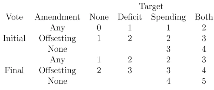
Government-spending-to-GDP ratio and deficit-to-GDP ratio Clearly, the questions investigate on four procedural rules: Vote on budget size (initial/final),Spending level target (present/absent),Deficit level target
(present/ absent), and Amendments (any/offsetting/none). These become the rules subject to our concern.
2.5
Budget process
First, let Nature select a winning coalition S ∈ G. The coalition members bargain over the budget irrespective of development in the legislature, so we may suppose an unconstrained Nash-bargaining solution (in Section 2.7.1, the coalition members begin to consider development in later stages when bargaining over coalitional contract):
[τS, γS] = argmax Y j∈S
Uj(τS, γS) τS ∈T γS ∈G, γS ≤2τS (8)
1. Fiscal targets. The coalitionS may agree on two aggregate level limits which are enforceable—Spending level (γ = γS) and/or Deficit level (b=bS, i.e. γ/τ =γS/τS) targets.
Then, the budget goes to the legislature.
2. Initial vote. There may be an initial simple-majority vote on the budget size γ (unless the spending level is already targeted).
3. Amendments. This procedure is left for Classic Case. In Basic Case, we consider only single public good γ without any internal structure and possibility of amendments.
4. Revenue side. The Parliament votes on tax revenues τ by simple ma-jority unless both the deficit level and spending level have been set (in that case, tax is set as a residual variable).
5. Final vote on the budget size. This node doesn’t realize if the vote has already taken place (see Node 2), or if the spending has been deter-mined residually by deficit target and tax revenues (in Nodes 1 and 4).
We assume status quo (provisory budget, or caretaker government) is prohibitively costly for all participants, so a fully specified budget is always accepted in the last node.
In Basic Case, we combine three binary variables (Vote, Deficit target, Spending target), which results in eight decision-making configurations. Ta-ble 1 describes the order of variaTa-bles to be agreed in each case. In brackets, residual variables are described.
Table 1: Decision-making nodes in Basic Case Vote/Target None Deficit Spending Both
Initial γ; τ(b) bS; γ(τ) γS;τ(b) γS, bS(τS) Final τ; γ(b) bS; τ(γ) γS;τ(b) γS, bS(τS)
2.6
Basic Case equilibria
Since we’ve got 8 finite extensive games, we apply backward induction and identify subgaperfect equilibria. To solve each subcase, a concept of me-dian party is crucial. We obtain that by analogy to the Meme-dian Voter The-orem by Black [2]. The theThe-orem states that a median individual is always decisive in electoral stage if policy is located in single dimension and pref-erences are single-peaked. Although we have a two-dimensional space here
and parties of different size, we can get a median party provided that de-cisions on either of τ and γ are made separately. This is, indeed, our case. The separation implies that a decision on one dimension is made after the other dimension is fixed. When fixing any first dimension, parties of course anticipate the subsequent decision constrained by the fixed dimension.
We need to analyze how median parties arise in single dimensions. First of all, recall simple majority of votes is required in all nodes of the budget process, so we use the quotaqSMV :=|P
i∈Nsi|+1. Consider first the subcase of the Initial vote/No target, when γ is set in the first step, τ in the second step, and the deficit level b is obtained residually (see also in Table 1). For γ fixed in the first step for some ¯γ, we get constrained optima in the second step τi∗(¯γ) for eachi∈N. We sort parties by the optimal tax constrained by fixed spending and look for a median player. Intuitively, median player has the property that no connected winning subset of parties can do without him or her. For simple majority voting (as in our budget process) such a player can be unique, or there can be two such players. If the player is unique, the legislature coordinates on his/her preferred tax. For two players we assume, without loss of generality, that the lower tax of the two is selected.
Definition 3 (Medians constrained on fixed levels) Let the median tax
constrained on fixed spending τMG :G→T be a function of ¯γ ∈G such that:
X l∈N τl∗(¯γ)<τMG(¯γ) sl < qSMV∧ ∃i∈N :τi∗(¯γ) = τ G M(¯γ)∧si + X l∈N τl∗(¯γ)<τMG(¯γ) sl≥qSMV
The median tax constrained on fixed deficit τMB :B →T be a function of
¯ b ∈B such that: X l∈N τl∗(¯b)<τB M(¯b) sl < qSMV∧ ∃i∈N :τi∗(¯b) = τMB(¯b)∧si+ X l∈N τl∗(¯b)<τB M(¯b) sl≥qSMV
The median spending constrained on fixed tax γMT :T →G be a function of τ¯∈T such that: X l∈N γl∗(¯τ)<γT M(¯τ) sl< qSMV∧ ∃i∈N :γi∗(¯τ) =γ T M(¯τ)∧si+ X l∈N γl∗(¯τ)<γT M(¯τ) sl ≥qSMV
Let us proceed with the example of Initial vote/No target. The im-portance of median function constrained on fixed level in the second step is anticipated as early as in the first step; in other words, players recognize that
the outcome in the second step cannot be conditioned by anything preced-ing, for such a promise/threat could not be enforced. (Note that the process ends after the second step, so nothing else but median tax constrained on spending can be credibly promised in the first step to those who decide on expenditures.) So, what is the equilibrium γ chosen in the first step? Since parties anticipate the second stage, they optimize on the set restricted as follows: τ = τMG(¯γ), τ ∈ T, γ ∈ G, γ ≤ 2τ. On that set, each party i has an optimum denoted as [τG
M(γT ∗ i ), γT
∗
i ]. So, it would be the first-best for each party to ensure that γT∗
i gets elected in the first step, because a tax the leg-islature selects on the basis of this spending is the best given the restrictions. However, since γT∗
i are located in a single dimension, it must be again the median player who will be decisive.
This case illuminates how agents in early stages use constraints in order to optimize in next stages. Notice that the median spending is constrained; not on what has happened, but on what is anticipated to happen. By the same token, we derive solutions also for other institutional configurations. For this, we find parties’ optima on the set restricted as follows: γ =γT
M(¯τ), τ ∈ T, γ ∈ G, γ ≤ 2τ. We write them as [τiG∗, γT
M(τ G∗
i )]. Notation reflects the order of votes (GT for γ;τ and TG for τ;γ).
Definition 4 (Medians constrained by anticipated responses) Define
γGT
M as the median spending constrained on anticipated τMG (i.e. median tax
constrained on fixed spending):
X l∈N γT∗ l <γ GT M sl < qSMV∧ ∃i∈N :γiT∗ =γ GT M ∧si+ X l∈N γT∗ l <γ GT M sl≥qSMV Let τT G
M be the median tax constrained on anticipated γMT (i.e. median
spending constrained on fixed tax):
X l∈N τG∗ l <τ T G M sl < qSMV∧ ∃i∈N :τiG∗ =τ T G M ∧si + X l∈N τG∗ l <τ T G M sl≥qSMV 2.6.1 Median identity
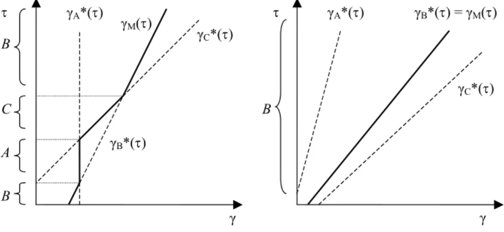
Note that a single median voter need not exist in an entire definition set when a median constrained on a fixed variable or a median constrained by anticipation is constructed. Simply, players in the early stages not only constrain sets for later stages, but also, at the same time, decide on who will be the next decisive player, which Figure 1 illustrates. On the figure, we have three functions of optimal spending constrained on fixed tax, each for one of
players A, B and C. The highlighted line is the function of median spending constrained on fixed tax. On the left side, we can see that for very low levels of τ, it is B who is decisive, while for higher values it is A or C. For the highest values, it is again B who becomes the median player. On the right side, we get the other case when only one player (B) is decisive regardless of decision on τ in the preceding stage, so we may call such a median function to be ‘one-player’. For example, the median tax constrained on spending is to be called ‘one-player’ as long as ∃i∈G,∀γ ∈ h0,2i:τi∗(γ) = τG
M(γ). Othwerwise, the median tax constrained on spending is a ‘many-player’ median function. By analogy, we would define one-player/many-player me-dian tax constrained on deficit as well as one-player/many-player meme-dian spending constrained on tax. Nonetheless, the fact that median players are different adds nothing extra to the problem of finding the subgame-perfect Nash equilibrium strategy profile; it is but an interesting element in the game.
γ τ γC*(τ) γB*(τ) γA*(τ) A B B C τ γC*(τ) γB*(τ) = γM(τ) γA*(τ) γ γM(τ) B
Figure 1: Many-player median spending vs. One-player median spending
2.6.2 Solutions in the general form
By backward induction, we obtain solution for any institutional configura-tion.
Initial vote/No target We have already described the solution in the
preceding subsection to be [τ,γ]=[τMG(γMGT),γMGT].
Final vote/No target In the second stage, we obtain γT
M(¯τ). Definition 3 has introduced tax demands for the first stage, constrained by anticipation of γT
Initial & Final vote/Deficit target The deficit contractually set at bS is fixing the relation between γ and τ such that γ =τ(1 +bS). The solution is therefore [τB
M(bS),(1 +bS)τMB(bS)].
Initial & Final vote/Spending target Suffice to use the median tax
constrained on fixed spending in order to arrive at the solution [τG
M(γS),γS].
Initial & Final vote/Both targets Obviously, the solution is [τS,γS].
2.6.3 Solutions in the specific form
In Section 4 dealing with effect of fragmentation, we employ explicit solutions to be applied in Basic Case, thereby making use of explicit assumptions from Section 2.1. With the exception of Initial vote/No target, we can derive them explicitly. Before doing that, we have to identify two median parties. Denote A = [αA, pA, sA] the party with median value of α and P = [αP, pP, sP] the party with median value of αi√pi:
X l∈N αl<αA sl < qSMV∧sA+ X l∈N αl<αA sl ≥qSMV X l∈N αl√pl<αP √ pP sl< qSMV∧sP + X l∈N αl√pl<αP √ pP sl ≥qSMV
These two median parties may be different but also identical (i.e. we may have a double-median party).
Proposition 3 Tax and spending in Basic Case are set as follows:
1. Final vote/No target case:
[τ, γ] = 1−αA, 2(1−αA) 1 + αP√pP
2. Initial & Final vote/Deficit target case:
[τ, γ] = 1−αA, γS(1−αA) τS
3. Initial & Final vote/Spending target case: [τ, γ] = [τM(γS), γS], where
τMG( ¯γS) = 1−αS+ αSγ¯S 2pS pS− 2τG M( ¯γS)−γ¯S ¯ γS αS
2.6.4 Illustration
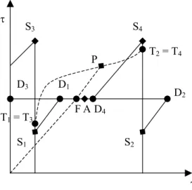
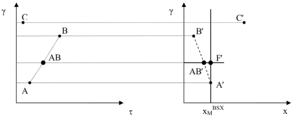
Outcomes put in Proposition 3 can be illustrated on four different coalitional contracts S1, . . . ,S4 in space T ×G. Figure 2 features the contracts as well as bliss points of median parties, A and P. Having coalitional contracts and median preferences, we are able to get solutions in each institutional con-figuration. For Final vote/No target subcase, we denote the solution as F (recall by Proposition 3, F is stable irrespective of coalition); it is the situ-ation when median parties A and P can exploit their power the most. The solutions for Deficit target subcase are D1, . . . ,D4 and for Spending target subcase T1, . . . ,T4. When both targets are set, the solutions are the initial contracts S1, . . . ,S4. S4 S3 P A T1 = T3 D1 D4 D2 D3 T2 = T4 F τ γ S1 S2
Figure 2: Solutions in Basic Case for 4 coalitions (S1, . . . ,S4)
The figure illuminates several facts. In the absence of fiscal governance, the median parties A and P can exploit their power and always establish F. When partial fiscal governance is present, solutions differ tremendously; the initial contract can be either utterly destroyed (T2 vs. S2), or only slightly compromised (T4 vs. S4). When fiscal governance is complete, coalitional contracts are perfectly stable and we get S1, . . . ,S4. The case D2 reflects the intuition in the title of the paper: parties “commit to deficit” and the spend-ing grows dramatically comparspend-ing to zero-governance mode F. By analogy, “committment to spendig effect” occurs in case of T2, when deficit is close to deficit in F, but spending significantly grows.
2.7
Endogenous coalitional contract
In the beginning, we assumed coalitional bargaining over an unrestricted space T × G, γ ≤ 2τ, which led to an unconstrained Nash-bargaining so-lution. However, the coalition parties know that in some configurations, their contract may be unsustainable. Why should they agree to a contract whose terms cannot be maintained? We shall distinguish between three cases. Firstly, if no part of the contract can be preserved, the contract is irrelevant (cheap talk), and coalitional agreement is irrelevant. Quite contrary, when parties commit to two targets, the contract is protected as the whole, so the unconstrained Nash-bargaining solution is stable.
The only analytically interesting extension emerges when the contract is partially unsustainable, which occurs when exactly one fiscal target (i.e. deficit or spending level) is subject to contract. We suggest here how to refine solutions of two cases on the grounds of the anticipation of partial unsustainability.
Initial & Final vote/Deficit target In the 2nd stage,τB
M(bS) is selected. Hence: bS = argmaxY j∈S Uj[τMB(b),(1 +b)τ B M(b)]
Initial & Final vote/Spending target In the 2nd stage, τG
M(γS) is se-lected. Hence: γS = argmaxY j∈S Uj[τMG(γ), γ]
3
Classic Case
The next step in the analysis of fiscal governance is to introduce different types of expenditures, which allows to tackle the effect of amendment rules. Suppose we have two public goods (with expenditure ratiox∈Gandw∈G) and all public good expenditures γ must be allocated into x and w so that x+w=γ.
To be able to analyze the system, we will assume Euclidean preferences in T ×G2, and thereby refrain from Cobb-Douglas utility function introduced in (5). We follow spatial approach to political economy which typically as-sumes Euclidean preferences, specifically in space T ×G (see Balassone and Giordano [1] as well as classic Ferejohn and Krehbiel [6]); because of that, we call the following model a Classic Case. The big disadvantage of Classic Case is that it is actually very difficult to realize how a realistic tax system
(e.g. one with proportional tax rate) and standard assumptions imposed on utility functions would result in circular preferences. For extensive discussion on spatial models encountering these limitations, see Milyo [10].
The main advantage of Euclidean preferences are algebraic properties which we intend to exploit here. For instance,τG
M(¯γ) andγMT (¯τ) are constants. In this section, we extend the spatial literature by postulating preferences in three-dimensional space, which we ensure through the following assumptions:
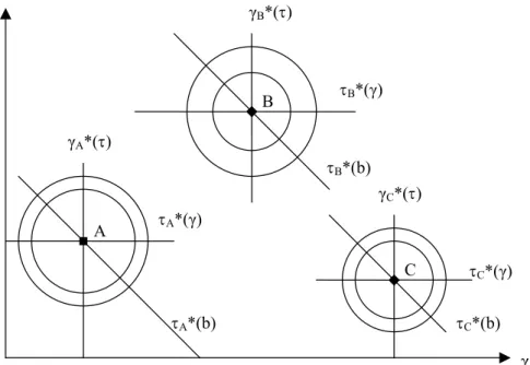
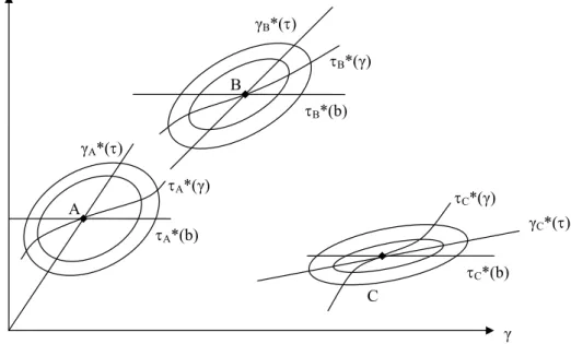
∀x= ¯x:Ui(τ,x, w¯ )−Ui(τi∗,x, w¯ ∗ i) = (τ−τ ∗ i) 2+ [w−(x∗ i +w ∗ i −x¯)] 2 ∀τ = ¯τ :Ui(¯τ , x, w)−Ui(¯τ , x∗i, w ∗ i) = 2(x−x ∗ i)2+2(x−x ∗ i)(w−w ∗ i)+(w−w ∗ i)2 This satisfies that circular preferences are achieved in subspaceT ×Gfor any xand in subspaceG2 for anyτ. Figures 3 and 4 reveal how Classic Case differs from Basic Case in subspace T ×G.
A B C τ γ γA*(τ) τA*(γ) τA*(b) τC*(b) τB*(b) τB*(γ) τC*(γ) γB*(τ) γC*(τ)
Figure 3: Utility functions in Classic Case
3.1
Institutional configurations
The division of budget into two public goods is a way to study amendment part of budgeting. If amendments are permitted, we assume that the first committee votes on x. Then, if there is no spending limit (imposed either
A B C τ γ γA*(τ) τA*(γ) τA*(b) τC*(b) τB*(γ) τC*(γ) γC*(τ) γB*(τ) τB*(b)
Figure 4: Utility functions in Basic Case
by targeted spending, initial vote or offsetting requirement), the second com-mittee votes on w. Otherwise, the second committee doesn’t vote. It is also possible that amendments are prohibited as such and no committee votes at all.
By combining three binary variables (Spending target, Deficit target, and Final vote) and one trinomial variable (Amendment), we study 24 institu-tional compositions instead of only 5 in Basic Case. However, in three cases when amendments are banned, total spending can differ from contracted γS, and it is necessary to define how the budgetary structure adjusts. This un-fortunately requires that amendment procedure must take place, so we skip these three cases as logically inconsistent. Furthermore, in some combina-tions we receive identical nodes, thus an identical game tree. Hence, we have in the end only 10 different node combinations (see Table 2).
Table 2: Decision-making nodes in Classic Case
Amendment Target
Initial vote None Deficit Spending Both
Any γ;x(w);τ bS;γ(τ);x(w) γS;x(w);τ bS;γS(τS);x(w) Offsetting γ;x(w);τ bS;γ(τ);x(w) γS;x(w);τ bS;γS(τS);x(w) None γS(xS, wS);τ bS;γS(τS, xS, wS)
Table 2: Decision-making nodes in Classic Case Final vote
Any x;w(γ);τ bS;x;w(γ, τ) γS;x(w);τ bS, γS(τS);x(w) Offsetting x;τ;γ(w) bS;x;τ(γ, w) γS;x(w);τ bS, γS(τS);x(w) None γS(xS, wS);τ bS;γS(τS, xS, wS) Our interest rests with the properties of fiscal governance indices, so we construct a basic index F ∈ {0, . . . ,5}, which is a sum of the Amendment part (0 for any, 1 for offsetting, 2 for none), Final vote part (0 for initial, 1 for final)3, and Targets (0 for none, 1 for deficit, 1 for spending, 2 for both). Table 3 comprises values of F for each institutional case.
Table 3: Fiscal governance index (F)
Target
Vote Amendment None Deficit Spending Both
Any 0 1 1 2 Initial Offsetting 1 2 2 3 None 3 4 Any 1 2 2 3 Final Offsetting 2 3 3 4 None 4 5
3.2
Classic Case equilibria
This section shows how to identify solutions for each mode of fiscal gover-nance when the budget is structured. We derive general solutions regardless of properties of utility function assumed in Classic Case so as to have a tool applicable beyond the scope of this paper. Doing so, we must introduce several new variables; notice that their notation always reflects the order of nodes. For instance, when the order of node is γ;x;τ, we use superscript GXT (for budget deficit target, we shall use B, and for spending target S).
3.2.1 Solutions in the general form
Initial vote/No target/Any & Offsetting amendments (GXT)
Solv-ing backwards, we firstly derive the tax. Optimal τ constrained on fixed 3In the case ofVote on budget size, we follow a non-intuitive result derived theoretically by Ferejohn and Krehbiel [6] and experimentally by Ehrhart et. al [5]: initial vote on global budget actually weakens the coalitional contract.
spending (as well as on fixed composition of spending) shall be found as τi∗|x=¯x,w= ¯w, with median value τMGXT(¯x,w¯). In the preceding (second) step, politicians set spending composition. They are constrained by fixed spending from the first step, and anticipated tax in the final step. Individual optima can be received by x∗i|γ=¯γ,τ=τGXT
M , with median valuex GXT M (¯γ).
Finally, we derive how spending is set in the anticipation of xGXTM (¯γ) and τGXT
M (¯x,w¯). We obtain individually optimal spending by optimizing γi∗|x=xGXT
M ,τ=τ
GXT
M , and the median is γ GXT
M . The solution we arrive at is [τ;γ;x] = [τGXT
M (γMGXT, xGXTM );γMGXT;xGXTM (γMGXT)].
Final vote/No target/Any amendment (XGT) Obviously,τMXGT(¯x,w¯) :=
τGXT
M (¯x,w¯). By analogy to the previous case, we derive γMXGT(¯x) and get the optimal value in the first step xXGTM .
The solution is [τ;γ;x] = [τMXGT(γMXGT, xXGTM );γMXGT(xXGTM );xXGTM ].
Final vote/No target/Offsetting amendment (XTG) By analogy, we
find γXTG
M (¯x,τ¯) for the third step. In the second step, we look for τMXTG(¯x), which allows to specify median value xXTG
M in the initial node. The solution is [τ;γ;x] = [τMXTG( ¯xXTG
M );γ XTG
M (xXTGM , τMXTG);xXTGM ].
Initial vote/Deficit target/Any & Offsetting amendments (BGX) Two variables are under control of the legislature. In the last step, parties select xBGX
M (¯γ, bS). The median spending in the preceding node is γMBGX(bS), and the solution writes [τ;γ;x] = [(1 +bS)γMBGX;γMBGX(bS);xBGXM (γMBGX, bS)].
Final vote/Deficit target/Any & Offsetting amendments (BXG) In the first step, parties choose x anticipating selection of γ in the second step. This case is very much similar to the previous case. We denote the median spending in the last step as γMBXG(¯x, bS). The median composition adopted in the previous step is xBXG
M (bS). We get the solution as follows: [τ;γ;x] = [(1 +bS)γMBXG;γMBXG(xBXGM , bS);xBXGM ]
Initial & Final vote/Spending target/Any & Offsetting
amend-ments (SXT) Like in the first two configurations, we seek for tax
con-strained by fixed spending and composition, thus τSXT
M (¯x,w¯) :=τMGXT(¯x,w¯). To find median decision on composition of spending, we simply insert γS and havexSXTM :=xGXTM (γS), so the solution is [τ;γ;x] = [τMSXT(γS, xMSXT);γS;xSXTM ].
Initial & Final vote/Spending target/No amendment (ST)
Obvi-ously, the solution is [τ;γ;x] = [τST
Initial & Final vote/Both targets/Any & Offsetting amendments
(BSX) The only variable set in the legislature is composition of spending,
reflecting pre-determinedγS and τS. We define median value simply asxBSXM and achieve solution [τ;γ;x] = [τS;γS;xBSXM ].
Initial & Final vote/Both targets/No amendments (BS) The
agree-ment of the coalition is preserved in total, and we receive [τ;γ;x] = [τS;γS;xS].
3.2.2 Illustration
Euclidean preference allow to provide the general solution in a very simple manner. This is to be illustrated on a special case. Suppose three parties (A, B, and C) are located in spaceT×G2 and Nature selects A+B as the winning coalition. Since majority of median functions constrained on fixed variables and median functions constrained by anticipation are constant, we derive solutions very easily. These are depicted in Figures 5–8 and summarized in Tables 4 and 5 as well as in Figure 9.
Table 4: Tax & Spending allocations Target
Vote Amendment No target Deficit Spending Both
Any D E F AB Initial Offsetting D E F AB None F AB Any D E F AB Final Offsetting D E F AB None F AB
Table 5: Budget structure Target
Vote Amendment No target Deficit Spending Both
Any D’ E’ F’ F’
Initial Offsetting D’ E’ F’ F’
None AB’ AB’
Any D’ E’ F’ F’
Final Offsetting D’ E’ F’ F’
τ γ C AB A B γ x AB′ A′ B′ C′ D γMGXT = γMXGT = γMXTG D′ xMGXT = xMXGT = xMXTG τMGXT = τMXGT = τMXTG Figure 5: No target (GXT, XGT, XTG) τ γ C AB A B γ x AB′ A′ B′ C′ E γMBGX = γMBXG xMBGX = xMBXG E′
Figure 6: Deficit target (BGX, BXG)
τ γ C AB A B γ x AB‘ A′ B′ C′ F γMST= γMSXT = γAB xMST xMSXT F′
τ γ C AB A B γ x AB′ A′ B′ C′ F′ xMBSX Figure 8: Both targets (BSX, BS)
τ γ C AB A B γ x AB′ A′ B′ C′ D D′ F E E′ F′ Figure 9: Summary
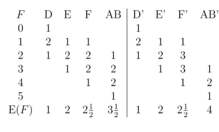
Interestingly, the index of fiscal governance again relates to final out-comes. The higher index, the closer is the outcome to the coalitional contract AB (AB’). Table 6 demonstrates this with frequencies and expected values of fiscal governance for each outcome. In other words, we observe that fiscal governance protects the coalitional contract like it did in Basic Case.
Table 6: Frequencies F D E F AB D’ E’ F’ AB’ 0 1 1 1 2 1 1 2 1 1 2 1 2 2 1 1 2 3 3 1 2 2 1 3 1 4 1 2 1 2 5 1 1 E(F) 1 2 212 312 1 2 212 4
4
Fragmentation
The effects of fragmentation on fiscal outcome have long been subject to intensive research, verifying mainly variants of CPR hypothesis (see Ric-cuitti [12] for perhaps the most recent contribution to the study of fiscal outcomes and fragmentation).
By CPR hypothesis, the more fragmented is the party system (measured by Herfindahl index), the stronger are incentives to exploit common pool, and worse fiscal outcomes. Moreover, highly fragmented systems suffer from a pronounced problem of collective action during the budget coordination, which makes the Finance Minister less reliable as a ‘non-partial’ budgetary coordinator. Hence, Hallerberg [8] recommends Commitment mode, includ-ing e.g. deficit and/or spendinclud-ing targets. To sum up, fiscal targets are quoted as the remedy exactly to the situations of fragmented party systems where fiscal costs are expected to abound.
In this section, we observe different results. In Proposition 3, we already found that fiscal targets increase fiscal volatility. From macroeconomic point of view, volatility is always costlier than stability, so despite reducing CPR incentives, fiscal targets keep extreme fiscal positions unchallenged, thereby amplify costs of fiscal volatility. Quite contrary, in the absence of targets, the budget rests in the position of median political agent regardless of frag-mentation and coalition composition.
We deal with two specifications. In the first one, the higher number of parties, the lower standard deviation of coalitional position from the globally
median position. As a result, costs of fiscal volatility increase in fiscal gover-nance but paradoxically decrease in fragmentation; both findings are in stark contrast to CPR hypothesis. In the second specification, the higher fragmen-tation, the bigger deviation of coalitional position from the global median. Here, fiscal volatility increases both in fiscal governance and fragmentation.
4.1
Fragmentation in
α
i(Basic Case)
4.1.1 Assumptions
Assume each party (citizen-candidate)i∈ {1, . . . , n}has preferences [αi, pi] = [αi, Kαi], where K is constant and a ∈ h0,1i. The citizen-candidates are drawn from the population such as to cover the dimension α in fixed dis-tances, i.e. αi+1−αi =αi−αi−1. This corresponds, among others, to a case of equal distribution of α∗i over spaceh0,1iand equal electoral support to all parties.
Assume also that only minimum-winning connected coalitions (MWC) can be formed. This might be justified by a small amount of rent distributed in an equal proportion to coalition members. The rent introduces an incentive to create small, namely minimum-winning coalitions. Furthermore, since the payment scheme is fixed, median members have reason to include parties which are connected in an existing coalition (here we can easily claim that a party x is connected to a coalition S if mini∈S(τi∗)≤τx∗ ≤maxi∈S(τi∗)).
We can represent preference of parties in a single dimension, because for preferences defined in our way, bliss points coordinates are functions of single variable α: τi∗ = 1−αi b∗i = 1−K 1 +K γ ∗ i = 2τi∗ 1 +K
For n parties, we need to divide the set h0,1i into n equal parts to satisfy the assumption of fixed distances. Doing so, we get preferences of party ias αi = (2i−1)/2n.
4.1.2 Coalitions
Consider simple-majority voting (q = sup(1/2)). Since party preferences can be expressed in single dimension α, we define coalitions by reference to this dimension. Define further the coalition size of S as maxi∈S(αi)−mini∈S(αi).
Odd number of parties Any MWC has to include (n + 1)/2 parties
we have (n + 1)/2 MWCs. A median position within the coalition j ∈ {1, . . . ,(n+ 1)/2}we write as αM
j = (4j +n−3)/4n.
Even number of parties Any MWC has to include (n+ 2)/2 parties to
win a simple-majority vote. Therefore, coalition size is 1/2 and we have n/2 MWCs. A median position within the coalition j ∈ {1, . . . , n/2} is αM
j = (4j+n−2)/4n.
Proposition 4 When party system includes odd number of parties, an
un-constrained coalitional contract of coalition j ∈ {1, . . . ,(n+ 1)/2} is as fol-lows: τj = 1−αjM = 3n+ 3−4j 4n γj = 3n+ 3−4j 2n(1 +K)
When the party system is even-sized, a coalitionj ∈ {1, . . . , n/2} selects:
τj = 1−αjM = 3n+ 2−4j 4n γj = 3n+ 2−4j 2n(1 +K) 4.1.3 Comparative statics
First of all, we check that an increase in number of parties doesn’t affect the average position of the coalition, i.e. there is no bias involved with the fragmentation.
Proposition 5 For party system of any size N, the expected coalitional
con-tract is E(τ) = 1/2.
Fragmentation brings a change to tax volatility, that we can measure by standard deviation of tax set in a coalitional contract.
Proposition 6 For odd number of parties andn >3, tax volatility decreases
in n. For even number of parties and n >2, tax volatility grows in n.
4.2
Interpretation
In traditional literature, fiscal targets serve to lower CPR incentives, and the need for targets becomes pronounced with higher fragmentation. Here we have a trade-off between CPR and volatility effect of fiscal governance for each level of fragmentation. In standard case (like in even-sized system we have introduced), higher fragmentation means higher volatility. Since higher fragmentation implies also the more pronounced CPR problem, we
cannot generally determine whether the optimal fiscal governance is stronger or weaker. In an alternative case (like the odd-sized system), volatility is smaller for highly fragmented system. Thus, the optimal fiscal governance is a stronger fiscal governance. This is in line with traditional literature on benefits of Committment mode for highly fragmented systems. However, we must remember that we reached this result only for a very special case.
5
Conclusion
The budgets in games we have modelled do not primarily suffer from alloca-tive inefficiencies of the common-pool type (CPR). The problem is the pure conflict of interest that cannot be overcome under given flat tax system and in the absence of compensations.
Fiscal governance appears to have two effects. In CPR, it works as a coordination device; in pure conflicts of fiscal preferences, it is a protection device. This ambiguity implies that strong fiscal governance both eliminates and magnifies fiscal costs of political fragmentation. The fact that multi-party governments find it easier to rely on Commitment mode, as Haller-berg [8] observes, not necessarily means motivation for efficiency, but for mutual protection.
To conclude, it may not be the case that the higher fiscal governance, the better fiscal policy.
References
[1] Balassone, F. and R. Giordano (2001), “Budget Deficits and Coalition Governments”, Public Choice, 106, 327-349.
[2] Black, D. (1958), The Theory of Committees and Elections, Cambridge: Cambridge University Press.
[3] De Haan, J., Moessen, W., and B. Volkerink (1999), “Budgetary Procedures—Aspects and Changes: New Evidence for Some European Countries”, in Poterba, J.M. and J. von Hagen (eds.), Fiscal Institu-tions and Fiscal Performance, Chicago and London: The University of Chicago Press, 265-299.
[4] Dharmapala, D. (2003), “Budgetary Policy with Unified and Decentral-ized Appropriations Authority”, Public Choice, 115, 347-367.
[5] Ehrhardt, K. et al. (2000), “Budget Process: Theory and Experimental Evidence”, ZEI Working Paper, B 18/2000.
[6] Ferejohn, J., and K. Krehbiel (1987), “The Budget Process and the Size of the Budget”, American Journal of Political Science, 31(2), 296-320. [7] Hallerberg, M. (2004), Domestic Budgets in a United Europe: Fiscal
Governance from the End of Bretton Woods to EMU. Ithaca, NY: Cor-nell University Press.
[8] Hallerberg, M. (1999), “Electoral Institutions, Cabinet Negotiations, and Budget Deficits in the European Union”, in Poterba, J. M. and J. von Hagen (eds.), Fiscal Institutions and Fiscal Performance, Chicago: The University of Chicago Press, 209-232.
[9] Imbeau, L. M. (2000), “The Political Economy of Public Deficits”, in Imbeau, L. M. and F. P´etry (eds.), Politics, Institutions, and Fiscal Policy: Public Deficits and Surpluses in Federated States, Lanham, MD: Lexington Books, 1-19.
[10] Milyo, J. (2000), “Logical Deficiencies in Spatial Models: A Constructive Critique”, Public Choice, 105, 273-289.
[11] Primo, D. M. (2004), “Institutional Constraints on U.S. State Spend-ing”, University of Rochester, mimeo.
[12] Ricciuti, R. (2004), “Political Fragmentation and Fiscal Outcomes”,
Public Choice, 118, 365-388.
[13] von Hagen, J. (1992), “Budgeting Procedures and Fiscal Performance in the European Community”, Economic Paper No. 96, Commission of the European Communities.
A
Proofs
Proof of Proposition 1 Part (i): Denote Qτ :=ycαcyˆ1−αc[(1 +δb)1−αc+
pcδ(1−b)1−αc]. The F.O.C. requires that in equilibrium: ∂Uc(αc, pc)
∂τc
=Qτ[(1−αc)(1−τc)αcτc−αc−αc(1−τc)αc−1τc1−αc] = 0 By eliminating strictly positive Qτ, we get αc/(1−αc) = (1−τc)/τc, which reduces toτc∗ = 1−αc. Secondly, we have to verify the second-order condition:
∂2Uc(αc, pc) ∂τ2 c = (αc−1)αc(1−τc)αc−2τc−(1+αc)(2τ 2 c −2τc+ 1)<0
By assumptions, the first term is strictly negative (α < 1), while the others are strictly positive (as to the last term, √D = √−4, so for all τ ∈ R the term is strictly positive).
Part (ii): Denote Qb := (1−τc)αcτc1−αcyαcc yˆ1−αc. Again, suffice to apply F.O.C.:
∂Uc(αc, pc) ∂bc
=Qbδ(1−αc)[(1 +δbc)−αc−pc(1−bc)−αc] = 0
Now, since Qb > 0, we obtain b∗c = (1− αc
√
pc)/(1 +δαc
√
pc). As usual, we verify the second-order condition:
∂2U i(αc, pc) ∂τ2 c =−αc 1 +δ 1 +δ αc√pc(δ+ αc√p c)<0
The first term is strictly negative (by assumption, αc >0), while the others are strictly positive (δ > 0 by assumption).
Part (iii): Sinceγ =τ(1 +b), we simply insert b∗:
γc∗ =τc∗(1 +b∗c) = 2(1−αc) 1 + αc√p
c
Proof of Proposition 2 Part (i): In order to get γi∗(¯τ), we apply F.O.C.:
∂Ui(αi, pi,τ¯) ∂τ =y αi i yˆ 1−αi (1−τ¯)(1−αi)[γ−αi−pi(2¯τ−γ)−αi] = 0
Since αi >0, we have ¯τ =τ∗ = 1−αi <1, so the root τ = 1 doesn’t apply. We put the last term equal zero and receive γi∗(¯τ) = 2¯τ /(1 + αi√pi). At last, we check that the second-order condition holds:
∂2Ui(αi, pi,τ¯)
∂γ2 =−αiγ
−αi−1−
piαi(2τ−γ)αi−1 <0
Very similarly, we derive b∗i(¯τ): ∂Ui(αi, pi,τ¯)
∂b =y αi i yˆ
1−αi
(1−αi)[(1 +b)−αi −pi(1−b)−αi]
By assumption, the first root α = 1 is not available, so we get the only one from the last term. Since τ is not present in the term, we clearly have b∗i(τ) = b∗i. The second condition is as follows:
∂2U
i(αi, pi,τ¯)
∂b2 =−αi(1 +b)
−αi−1−
Part (ii): So far, we have not explicit solution of τi∗(¯γ).
Part (iii): Like in Proof of Proposition 1, Part (i), the F.O.C. necessary to derive τi∗(¯b) is given as:
∂Ui(αi, pi,¯b)
∂τ =Qτ[(1−αi)(1−τ)
αiτ−αi−
αi(1−τ)αi−1τ1−αi] = 0
The solution is then the same, namely τi∗(¯b) = 1−αi. Also the second-order condition, already verified in Proof of Proposition 1, is identical.
Proof of Proposition 3 Part (i) (Final vote/No target): By backward
induction, we start in the final (second) step. From Proposition 2, we can see γi∗|τ=¯τ is a linear transformation of αi
√
pi. A linear trasformation of a distribution doesn’t change the identity of the median, so we get γT
M(¯τ) is a one-player function of median player P.
γMT (¯τ) = 2¯τ 1 + αP√pP Define QP := 2/(1 + αP
√
pP) for simplicity. By entering γMT (¯τ) into the utility function (6), we get Ui = (1−τ)αiτ1−αi[Q
1−αi
P +p(2−QP)1−αi], where by Proposition 1 the solution is τi∗ = 1−αi. Obviously, the median τMT G is given by median αA, hence τMT G= 1−αA.
Part (ii) (Deficit target): By Proposition 2, we know τi|b=¯b = 1 −αi. Thus, τMB = 1−αA. Since b = bS and b = (γ −τ)/τ = γ/τ −1, we have γ/τ =γS/τS. Accordingly, γMB =γSτMB/τS.
Part (iii) (Spending target): Since γ =γS, we look for a median of τi∗|γS as expressed in Proposition 2: τMG(γS) = 1−αS+ αSγ¯S 2pS pS − 2τG M( ¯γS)−γ¯S ¯ γS αS
Part (iv) (Both targets): An unconstrained Nash-bargaining outcome [τS, γS] is preserved here as the whole.
Proof of Proposition 4 Part (i). First of all, we obtain a coalitional
contract for any coalition S. Nash-bargaining solution requires that (τS, bS) satisfies:
(τS, bS) = argmax Y i∈S
Ui(τS, bS)
Since b is constant, suffice to seek τS. We can rewrite: Y i∈S Ui(τS) = (1−τS) P i∈Sαiτ1− P i∈Sαin S Y i∈S [(1 +b)1−αi+pi(1−b)1−αi]
By F.O.C., we get τS = 1− P
i∈S αi
n = 1−ES(α).
Part (ii). Consider the odd number first. In each coalitionj ∈ {1, . . . ,n+12 }, we have (n+ 1)/2 parties. Each party i within the coalition we can repre-sent by αi such that i ∈ {j, . . . , j+ n−12 }. Before we express Ej(αi), we use Pa
i=0 = a(a+1)
2 to compute the following auxiliary expression: j+n−21 X i=j i= j(n+ 1) 2 + n−1 2 X i=0 i= (n+ 1)(4j+n−1) 8
Now we easily deriveEj(α) and see that tax preferred by median position is the Nash-bargaining solution for the coalition.
Ej(α) = 2 n+ 1 j+n−21 X i=1 2i−1 2n = 2 n+ 1 Pj+n−21 i=1 i n − n+ 1 4n ! = 4j +n−3 4n
Part (iii). Consider the even-sized system. In each coalitionj ∈ {1, . . . ,n2}, we have (n+ 2)/2 parties. Each party i within the coalition we can repre-sent by αi such that i ∈ {j, . . . , j + n2}. Again, we compute an auxiliary expression: j+n 2 X i=j i= j(n+ 2) 2 + n 2 X i=0 i= (n+ 2)(4j+n) 8
Now we easily derive Ej(α) and again confirm that tax preferred by me-dian position is the Nash-bargaining solution for the coalition.
Ej(α) = 2 n+ 2 j+n2 X i=1 2i−1 2n = 2 n+ 2 Pj+n2 i=1 i n − n+ 2 4n ! = 4j+n−2 4n
In both cases, we get Ej(α) = αMj , and τj =τjM.
Proof of Proposition 5 Part (i). Let us express the expected value of τ
for any n: E(τ) = 1−E(αM) = 1− n+1 2 X j=1 2(4j+n−3) (n+ 1)4n = 1 2
Part (ii). Similarly, the expected value of τ for any n writes as E(τ) = 1−E(αM) = 1−Pn2 j=1 2(4j+n−2) n(4n) = 1 2.
Proof of Proposition 6 We shall compute variance at first, given as Var(τ) = E(τ −E(τ))2 = E(α −1/2)2. In finding variance, we apply a rule Pai=0i2 =a(a+ 1/2)(a+ 1)/3.
Part (i). For odd size, the variance is as follows:
Var(τ) = E 4j −n−3 4n 2 = n 2+ 6n+ 9 16n2 + n+1 2 X j=1 2j2 n2(n+ 1)− −n n+1 2 X j=1 j n2(n+ 1) −3 n+1 2 X j=1 j n2(n+ 1) = n2+ 2n−3 48n2
To check how volatility depends on fragmentation, we analyze the slope of standard deviation in n, i.e the first derivative of square root of variance:
∂pVar(τ) ∂n =
3−n
4n2p3(n2+ 2n−3
For n > 3, the term is negative which means that fiscal volatility decreases in fragmentation.
Part (ii). For even size of the party system, we get:
Var(τ) = E 4j −n−2 4n 2 = n 2+ 4n+ 4 16n2 + n 2 X j=1 2j2 n3 −n 2 n 2 X j=1 j− 2 n3 n 2 X j=1 j = n 2−4 48n2
Again, analyze the first derivative of square root of variance: ∂pVar(τ)
∂n =
1 p
3(n2 −4)
Forn >2, the term is positive and we can state that fiscal volatility increases in fragmentation.
Previously published:
2003:
26. Ondřej Schneider : European Pension Systems and the EU Enlargement
27. Martin Gregor: Mancur Olson redivivus, „Vzestup a pád národů“ a současné společenské vědy” 28. Martin Gregor: Mancur Olson’s Addendum to New Keynesianism: Wage Stickiness Explained 29. Patrik Nový : Olsonova teorie hospodářského cyklu ve světle empirie: návrh alternativního
metodologického přístupu
30. Ondřej Schneider: Veřejné rozpočty v ČR v 90. letech 20. století – kořeny krize 31. Michal Ježek: Mikroanalýza reformy českého důchodového systému
32. Michal Hlaváček: Efektivnost pořízení a předávání informace mezi privátními subjekty s pozitivně-extenalitní vazbou
33. Tomáš Richter: Zástavní právo k podniku z pohledu teorie a praxe dluhového financování
34. Vladimír Benáček: Rise of an Authentic Private Sector in an Economy of Transition: De Novo Enterprises and their Impact on the Czech Economy
35. Tomáš Cahlík, Soňa Pokutová, Ctirad Slavík: Human Capital Mobility 36. Tomáš Cahlík, Jakub Sovina: Konvergence a soutěžní výhody ČR 37. Ondřej Schneider, Petr Hedbávný: Fiscal Policy: Too Political? 38. Jiří Havel: Akcionářská demokracie „Czech made“
39. Jiří Hlaváček, Michal Hlaváček: K mikroekonomickému klimatu v ČR na začátku 21.století: kartel prodejců pohonných hmot? (případová studie)
40. Karel Janda: Credit Guarantees in a Credit Market with Adverse Selection 41. Lubomír Mlčoch: Společné dobro pro ekonomiku: národní, evropské, globální 42. Karel Půlpán: Hospodářský vývoj Německa jako inspirace pro Česko
43. Milan Sojka: Czech Transformation Strategy and its Economic Consequences: A Case of an Institutional Failure
44. Luděk Urban: Lisabonská strategie, její hlavní směry a nástroje. 2004:
45. Jiří Hlaváček, Michal Hlaváček: Models of Economically Rational Donators 46. Karel Kouba, Ondřej Vychodil, Jitka Roberts: Privatizace bez kapitálu.
47. František Turnovec: Economic Research in the Czech Republic: Entering International Academic Marke.t 48. František Turnovec, Jacek W. Mercik, Mariusz Mazurkiewicz: Power Indices: Shapley-Shubik or
Penrose-Banzhaf?
49. Vladimír Benáček: Current Account Developments in Central, Baltic and South-Eastern Europe in the Pre-enlargement Period in 2002-2003
50. Vladimír Benáček: External Financing and FDI in Central, Baltic and South-Eastern Europe during 2002-2003
51. Tomáš Cahlík, Soňa Pokutová, Ctirad Slavík: Human Capital Mobility II
52. Karel Diviš, Petr Teplý: Informační efektivnost burzovních trhů ve střední Evropě
53. František Turnovec: Česká ekonomická věda na mezinárodním akademickém trhu: měření vědeckého kapitálu vysokoškolských a dalších výzkumných pracovišť
54. Karel Půlpán: Měnové plánování za reálného socialismu
55. Petr Hedbávný, Ondřej Schneider, Jan Zápal: Does the Enlarged European Union Need a Better Fiscal Pact?
56. Martin Gregor: Governing Fiscal Commons in the Enlarged European Union.
57. Michal Mejstřík: Privatizace, regulace a deregulace utilit v EU a ČR: očekávání a fakta
58. Ilona Bažantová: České centrální bankovnictví po vstup České republiky do Evropské unie (právně institucionální pohled)
59. Jiří Havel: Dilemata českého dozoru finančních trhů.
61. Karel Janda: Bankruptcy Procedures with Ex Post Moral Hazard
62. Ondřej Knot, Ondřej Vychodil: What Drives the Optimal Bankruptcy Law Design
63. Jiří Hlaváček, Michal Hlaváček: Models of Economically Rational Donators: Altruism Can Be Cruel 64. Aleš Bulíř, Kateřina Šmídková: Would Fast Sailing towards the Euro Be Smooth? What Fundamental Real
Exchange Rates Tell Us about Acceding Economies?
65. Gabriela Hrubá: Rozložení daňového břemene mezi české domácnosti: přímé daně 66. Gabriela Hrubá: Rozložení daňového břemene mezi české domácnosti: nepřímé daně
67. Ondřej Schneider, Tomáš Jelínek: Distributive Impact of Czech Social Security and Tax Systems: Dynamics in Early 2000’s.
68. Ondřej Schneider: Who Pays Taxes and Who Gets Benefits in the Czech Republic? 2005:
69. František Turnovec: New Measure of Voting Power
70. František Turnovec: Arithmetic of Property Rights: A Leontief-type Model of Ownership Structures 71. Michal Bauer: Theory of the Firm under Uncertainty: Financing, Attitude to Risk and Output Behaviour 72. Martin Gregor: Tolerable Intolerance: An Evolutionary Model
73. Jan Zápal: Judging the Sustainability of Czech Public Finances
74. Wadim Strielkowsi, Cathal O’Donoghue: Ready to Go? EU Enlargement and Migration Potential: Lessons from the Czech Republic in the Context of the Irish Migration Experience
75. Roman Horváth: Real Equilibrium Exchange Rate Estimates: To What Extent Are They Applicable for Setting the Central Parity?
76. Ondřej Schneider, Jan Zápal: Fiscal Policy in New EU Member States: Go East, Prudent Man 77. Tomáš Cahlík, Adam Geršl, Michal Hlaváček and Michael Berlemann: Market Prices as Indicators of
Political Events- Evidence from the Experimental Market on the Czech Republic Parliamentary Election in 2002
78. Roman Horváth: Exchange Rate Variability, Pressures and Optimum Currency Area Criteria: Implications for the Central and Eastern European Countries
79. Petr Hedbávný, Ondřej Schneider, Jan Zápal: A Fiscal Rule That Has Teeth: A Suggestion for a “Fiscal Sustainability Council” Underpinned by the Financial Markets
80. Vít Bubák, Filip Žikeš: Trading Intensity and Intraday Volatility on the Prague Stock Exchange: Evidence from an Autoregressive Conditional Duration Model
81. Peter Tuchyňa, Martin Gregor: Centralization Trade-offs with Non-Uniform Taxes
82. Karel Janda: The Comparative Statics of the Effects of Credit Guarantees and Subsidies in the Competitive Lending Market
83. Oldřich Dědek: Rizika a výzvy měnové strategie k převzetí eura
84. Karel Janda, Martin Čajka: Srovnání vývoje českých a slovenských institucí v oblasti zemědělských finance 85. Alexis Derviz: Cross-border Risk Transmission by a Multinational Bank
86. Karel Janda: The Quantitative and Qualitative Analysis of the Budget Cost of the Czech Supporting and Guarantee Agricultural and Forestry Fund
87. Tomáš Cahlík, Hana Pessrová: Hodnocení pracovišť výzkumu a vývoje
Univerzita Karlova v Praze, Fakulta sociálních věd
Institut ekonomických studií [UK FSV – IES] Praha 1, Opletalova 26