Flow physics and sensitivity to RANS modelling
assumptions of a multiple shock wave/turbulent
boundary layer interaction
K. Boycheva,1, G. N. Barakosa,2, R. Steijla,3
aCFD Laboratory, School of Engineering, University of Glasgow, G128QQ, Glasgow, UK
Abstract
Reynolds Averaged Navier Stokes simulation (RANS) using the in-house CFD solver of Glasgow University is utilized to investigate the flow physics
and the sensitivity to modelling assumptions of a multiple shock wave tur-bulent boundary layer interaction in a rectangular duct (Mr = 1.61, Reδr =
162000). Such interactions often occur in high-speed intakes. Two-dimensional simulations were first performed to investigate the required grid resolution.
Then the sensitivity of the solution to different turbulence models is con-sidered. Based on the required grid resolution a series of three-dimensional
simulations were performed to investigate the effect of spanwise confinement and turbulence models. Lastly, using the best approach based on the above
investigations, results from two additional test cases were compared to their experiments, and conclusions are drawn as to the best way to simulate
mul-Email addresses: [email protected](K. Boychev),
[email protected](G. N. Barakos),[email protected](R. Steijl)
1PhD Student, CFD Laboratory, School of engineering
2Professor, MAIAA, MRAes, CFD Laboratory, School of engineering 3Senior Lecturer, CFD Laboratory, School of engineering
tiple shock wave turbulent boundary layer interactions.
Keywords: pseudo shock, shock train, shock wave boundary layer
interaction, SWBLI, MSWBLI, corner flow
1. Introduction
When the flow past an object travelling at high velocity becomes super-sonic, shock waves inevitably form, caused either by a change in the slope of
a surface, a downstream obstacle, or back pressure forcing the flow to become subsonic. The interaction of a shock wave with a boundary layer (SWBLI)
occurs in a variety of devices such as supersonic wind tunnel diffusers and supersonic (high-speed) intakes.
Flow p0 T0 2h Mr, δr p p M<1
Figure 1: Sketch of the re-acceleration process for multiple SWBLI
Of particular interest are SWBLIs in supersonic intakes. Supersonic
in-takes usually feature one or several compression ramps, forming a supersonic compression region trough oblique SWBLIs. The supersonic compression region ends with a terminal shock, which during critical operation of the in-take is located at the inin-take throat. The state of the boundary layer ahead of the terminal shock may lead to the formation of multiple SWBLIs in the intake throat. These multiple SWBLIs are often referred to as shock-trains
or pseudo-shocks. Although these terms are used interchangeably, the term
shock-train refers to the series of shocks and the pseudo-shock term refers to the entire region of pressure rise (Matsuo et al. [1]). Figure 1 illustrates
the basic physics of a multiple SWBLI interaction.For the multiple SWBLI, sketched in figure 1, the first shock imparts an adverse pressure gradient
on the incoming boundary layer developing on the top and bottom walls of a channel. If the adverse pressure gradient is large enough, the boundary
layer may separate and a recirculating flow region may form. This region leads to the formation of oblique compression shocks (leading and trailing
legs) which eventually join with the first shock to form a λ shock structure. From the bifurcation (or triple) point a secondary shear layer can develop
in the form of a slip line. Downstream the first shock, the flow is subsonic, however, the local streamline curvature re-accelerates the flow. Due to the
curvature, the supersonic flow downstream of the trailing leg of the shock is turned towards the wall. The turning of the flow forms a ”diamond-shaped”
re-acceleration region. Depending on how sudden the turn is towards the wall (governed by the flow confinement δr/h) the flow may again become
supersonic and promote the formation of multiple SWBLIs. By performing simulations of flows with multiple SWBLIs, investigating the sensitivities of
the problem to modelling assumptions, and by comparing the results with high-fidelity simulations and experiments we might gain a better insight of
the governing physics of multiple SWBLIs and the possible shortcomings of eddy-viscosity based turbulence models for such flows. Currently, the most
comprehensive normal MSWBLI experiments suitable for validation of CFD software are atMr = 1.61 andReδr = 162000, and were performed by Carroll
& Dutton. [2, 3, 4, 5, 6, 7]. Therefore, we target their experiment for CFD
validation. The experiment features not only wall pressure and centreline Mach number measurements but also mean velocity and velocity statistics
obtained through laser Doppler velocimetry (LDV). Two additional cases suitable for validation are also considered. The first is an experiment by Sun
et al. [8] of a normal MSWBLI in a rectangular test section at Mr= 2.0 and
Reδr = 250000. The Mach and the Reynolds numbers are higher than for
the experiment by Carroll et al. [2, 3, 4, 5, 6, 7]. The second is a numerical simulation by Fi´evet et al. [9, 10] of a normal MSWBLI in a rectangular
test section at Mr = 2.0 and Reδr = 34736 approximating the experiment by Klomparens et al. [11, 12]. The Reynolds number of this experiment is
an order of magnitude lower than the one in the other experiments, making it suitable for scale-resolving simulations. Other investigations of MSWBLIs
include the experiments by Weiss et al. [13] and Gawehn et al. [14]. Several scale-resolving simulations of the normal MSWBLI experiment by Carroll
et al. [2, 3, 4, 5, 6, 7] were performed by Morgan et al. [15, 16], Vane et al. [17], and Roussel et al. [18]. The simulations were performed at low
Reynolds number, an order of magnitude less than the experiments due to the computational restrictions of the employed methods. In section 2 we
present a brief discussion of the numerical method used in the present work. The computational setup including a description of the various simulations
performed is then described in section 3. Results are presented in section 4 focusing first on the the experiment by Carroll et al. [2, 3, 4, 5, 6, 7].
Two and three-dimensional simulations of the Mr = 1.61 and Reδr = 162000 MSWBLI are presented and compared with experiments. Following these
results, further simulations of the other two MSWBLI cases - by Sun et al.
[8] and Fi´evet et al. [9, 10] are presented, briefly.
2. Numerical method
The Helicopter Multi-Block (HMB3) [19, 20] code is used in the present
work. HMB3 solves the Unsteady Reynolds Averaged Navier-Stokes (URANS) equations in integral form using the Arbitrary Lagrangian Eulerian (ALE)
formulation for time-dependent domains, which may include moving bound-aries. The Navier-Stokes equations are discretised using a cell-centred finite
volume approach on a multi-block grid. The spatial discretisation of these equations leads to a set of ordinary differential equations in time
d
dt(Wi,j,kVi,j,k) = −Ri,j,k(Wi,j,k) (1)
where i,j,k represent the cell index, W andR are the vector of conservative
flow variables and flux residual respectively, and Vi,j,k is the volume of the celli,j,k. To evaluate the convective fluxes Osher [21] approximate Riemman
solver is used, while the viscous terms are discretised using a second order central differencing spatial discretisation. The Monotone Upstream-centered
Schemes for Conservation Laws, which is referred to in the literature as the MUSCL approach and developed by Leer [22], is used to provide high-order
accuracy in space. The HMB3 solver uses the alternative form of the Albada limiter [23] being activated in regions where large gradients are encountered
mainly due to shock waves, avoiding the non-physical spurious oscillations. An implicit dual-time stepping method is employed to perform the
achieve a fast convergence, which is solved using a first-order backward
dif-ference. The linearized system of equations is solved using the Generalised Conjugate Gradient method with a Block Incomplete Lower-Upper (BILU)
factorisation as a pre-conditioner [24]. To allow an easy sharing of the calcu-lation load for a parallel job, multi-block structured grids are used. Various
turbulence models are available in the HMB3 solver, including several one-equation, two-one-equation, three-one-equation, and four-equation turbulence
mod-els. Furthermore, Large-Eddy simulation (LES), Detached-Eddy Simulation (DES), and Delayed-Detached-Eddy Simulation (DDES) are also available.
In the present work the fully-turbulent standard k−ω by Wilcox [25], base-line k-ω by Menter [26], k−ω SST by Menter [26], and k−ω EARSM by Hellsten, Wallin, and Johansson [27, 28] turbulence models are used. Limited results with DES are used to illustrate the resolution of the flow offered by
RANS methods.
3. Numerical setup
3.1. Description of the target experiment
For all simulations performed we target for comparison the multiple SWBLI
experiment by Carroll & Dutton [2, 3, 4, 5, 6, 7]. Figure 2 shows a schematic of the experimental setup.
In the experiment, a 750 mm long rectangular test section was used with LDV measurements beginning atxr= 264.8 mm (the approximate location of
the first normal shock), and extending downstream at variable intervals over 400 mm. The top and bottom wall of the rectangular test section had a
xr x=xu=0 753.8 mm 400 mm 264.8 mm Stagnation chamber Nozzle Test section
Figure 2: Sketch of the experimental setup of the MSWBLI experiment by Carroll & Dutton [2, 7]
and height of the rectangular test section at x = 264.8 mm is 2h = 33.75
mm andw= 76.2 mm. Over the length of the LDV measurements, both the upper and lower wall diverge by 0.91 mm. Simulations of the flow are
per-formed at the experimental Reynolds number of Reδr = 162000. As pressure
measurements at the core of the flow are not available, the pressure at the outlet is assumed constant in the wall-normal and spanwise direction, equal to the wall pressure measured at that location. This assumption was used as pressure was measured only at a single location (at the wall). Computa-tional domains of 753.8 mm in length are simulated extending from an inlet
coincident with x= 0 mm. Figure 3 shows a schematic of the domain. Since measurements are provided at xr = 264.8 mm (δr = 5.4 mm, δr/h= 0.32),
the computational domain had a height of 2h = 33.75 mm at xr. To fully define the domain geometry the divergence angle of 0.13 deg is taken into
ac-count, and it is ensured that over the length of the LDV measurements (400 mm) the upper and lower walls diverge by 0.91 mm. Since measurements at
the inlet of the test section are not available, the inlet Mach number Mu and the outlet pressure ratio p/pu are adjusted so that the pre-shock Mach
num-ber is Mr = 1.61 and also the confinement ratio is δr/h= 0.32, downstream
of the inlet. Previous work by Morgan et al. [15, 16] shows that the location of the first shock, xr, varies dramatically with different turbulence models
for fixedMu andp/pu. In addition to the variation of the location of the first shock, different turbulence models predicted different first shock structures
and in general were found to overpredict the separation. Only in the work of Morgan [29] velocity profiles and Reynolds stresses from the RANS
simula-tions were compared to the results from a scale-resolving simulation (LES). The current work makes detailed comparisons of the streamwise velocity,
wall-normal velocity, turbulent kinetic energy, and Reynolds stresses in an attempt to quantify the sensitivity of the MSWBLI to different modelling
assumptions and suggest the best approach to simulating MSWBLIs.
Iu,Mu,pu,δu Flow p Mr, δr,pr 753.8 mm x y 0.26° 33.75 mm (2h) 400 mm 264.8 mm LDV Region xr xu
Figure 3: Sketch of the numerical setup of the MSWBLI experiment by Carroll & Dutton [2, 7]
3.2. Overview of Simulations
3.2.1. Preliminary two-dimensional RANS
To establish a reasonable baseline for comparisons, and to determine the
required grid resolution a series of two-dimensional RANS simulations were first performed. A uniform profile for the flow variables was specified at
Table 1: Grid parameters for the two-dimensional RANS simulations; Brackets indicate spacing in wall units
Parameter/Grid Coarse Medium Fine min ∆x/h 0.038 (380) 0.018 (180) 0.008 (80) max ∆x/h 0.3 (3×10⁴) 0.3 (3×10⁴) 0.3 (3×10⁴) min ∆y/h 1.0×10⁻⁵(0.1) 1.0×10⁻⁵(0.1) 1.0×10⁻⁵(0.1) max ∆y/h 0.05 (500) 0.05 (500) 0.05 (500) min ∆z/h 1.0×10⁻⁵(0.1) 1.0×10⁻⁵(0.1) 1.0×10⁻⁵(0.1) max ∆z/h 0.05 (500) 0.05 (500) 0.05 (500) Points 2.16×10⁵ 3.64×10⁵ 6.42×10⁵
ratio were set to Mu = 1.64, Iu = 0.01 (1 %), and µtµ = 10. Adiabatic wall boundary conditions were imposed at the y/h=−1 and y/h= 1 boundaries of the domain, and first-order extrapolation on all variables (except pressure where the flow is subsonic) was used at the outlet. Three grids were used
to investigate the sensitivity of the solution to grid refinement. Table 1 lists the grid parameters. The domain was discretised with 152 cells along
its height 2h. The boundary layers were resolved using at least 40 cells in the wall-normal direction and a non-dimensional distance of y+ ≤ 1 at the
wall was ensured. To achieve grid convergence, the grid was refined in the streamwise direction. The coarse, medium, and fine grids had the same y
-and z- resolution but 714, 1199, and 2113 cells in the x- direction. Table 2 lists the simulations parameters. Both the quantities at the inlet (subscript
u) and at the start of the interaction (subscript r) are reported in the table and compared to the experiment. Experimental measurements begin at the
location of the start of the interaction. All simulations were initialized with a normal shock of strength Mu at the end of the domain, and were allowed
Table 2: Two-dimensional RANS simulations parameters
Grid Iu% Mu Mr δrmm δr/h xr/h p/pu p/pr Turbulence model Coarse 1.0 1.640 1.614 6.3567 0.3906 26.6968 2.4841 2.3773 k-ωSST Medium 1.0 1.640 1.614 6.6089 0.4061 27.5227 2.4841 2.3756 k-ωSST Fine 1.0 1.640 1.612 6.6936 0.4113 27.7206 2.4841 2.3722 k-ωSST Fine 1.0 1.640 1.606 7.8263 0.4809 32.2001 2.4841 2.3460 k-ω Fine 1.0 1.640 1.610 7.3689 0.4528 32.9220 2.4841 2.3764 k-ωBSL Fine 1.0 1.640 1.622 5.0564 0.3107 26.6500 2.4841 2.4094 k-ωEARSM Experiment [2] - - 1.610 5.4000 0.3200 0 - 2.2309 -3.2.2. Three-dimensional RANS
Following the two-dimensional RANS simulations and the established grid
resolution required to accurately capture the normal MSWBLI a series of three-dimensional RANS simulations were performed to investigate the effect
of spanwise flow confinement on the solution. Simulations were performed on a three-dimensional grid having the same aspect ratio as in the experiment.
In a normal MSWBLI experiment in a constant area duct, Handa et al. [30] found the time-averaged flow to be mostly symmetric about the centre
planes. However, such symmetry should not be expected for shock trains at higher Mach numbers. Since the Mach number upstream of the first shock
in the experiment by Carroll et al. [2, 3, 4, 5, 6, 7] was Mr = 1.61 it was of interest to examine whether the flow was symmetric. Potential savings in
computational resources can be achieved if only a quarter of the domain is simulated. The domain was discretised with 76 cells along its height h and
98 cells along its width w. The fine grid and veryfine grids resulted in y+
of approximately 0.05 at the wall, taken at the location of the onset of the
interaction. Table 3 lists the grid parameters.
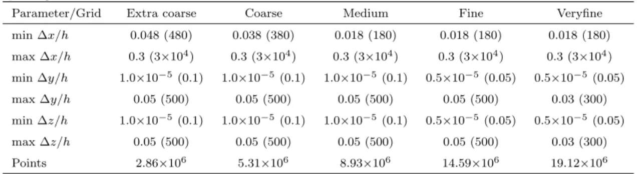
Table 3: Grid parameters for the three-dimensional RANS simulations; Brackets indicate spacing in wall units
Parameter/Grid Extra coarse Coarse Medium Fine Veryfine min ∆x/h 0.048 (480) 0.038 (380) 0.018 (180) 0.018 (180) 0.018 (180) max ∆x/h 0.3 (3×10⁴) 0.3 (3×10⁴) 0.3 (3×10⁴) 0.3 (3×10⁴) 0.3 (3×10⁴) min ∆y/h 1.0×10⁻⁵ (0.1) 1.0×10⁻⁵ (0.1) 1.0×10⁻⁵ (0.1) 0.5×10⁻⁵ (0.05) 0.5×10⁻⁵ (0.05) max ∆y/h 0.05 (500) 0.05 (500) 0.05 (500) 0.05 (500) 0.03 (300) min ∆z/h 1.0×10⁻⁵ (0.1) 1.0×10⁻⁵ (0.1) 1.0×10⁻⁵ (0.1) 0.5×10⁻⁵ (0.05) 0.5×10⁻⁵ (0.05) max ∆z/h 0.05 (500) 0.05 (500) 0.05 (500) 0.05 (500) 0.03 (300) Points 2.86×10⁶ 5.31×10⁶ 8.93×10⁶ 14.59×10⁶ 19.12×10⁶
streamwise direction. The coarse and medium grids had the same y− and
z− resolution (76 and 98 cells), but 714 and 1199 cells in the x− direction (both having the same resolution as the 2D coarse and medium grids). In addition a fine grid with reduced min ∆y/h and ∆z/h and a veryfine grid
with reduced min and max ∆y/h and ∆z/h was considered. Lastly, an extra coarse grid with and without symmetry was used to check if the flow
exhibits symmetry. Simulations were performed on all grids with the k-ω
SST turbulence model. Additional simulations on the medium grid with the
k-ω [26], baseline k-ω [26] and k-ω EARSM [27, 28] turbulence models were performed. Table 4 lists the simulation parameters. Both the quantities
at the inlet (subscript u) and at the start of the interaction (subscript r) are reported in the table and compared to the experiment. Experimental
measurements begin at the location of the start of the interaction. Again, all simulations were initialized with a normal shock of strength Mu at the end
of the domain and were allowed to converge to at least 5 orders of magnitude in the flux residuals.
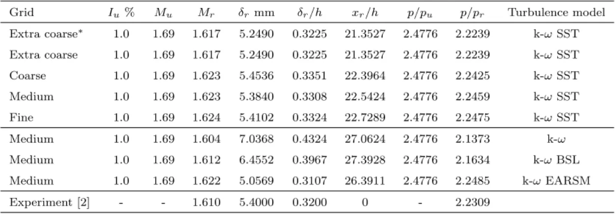
Table 4: Three-dimensional RANS simulations parameters;∗-grid without symmetry Grid Iu% Mu Mr δr mm δr/h xr/h p/pu p/pr Turbulence model Extra coarse∗ 1.0 1.69 1.617 5.2490 0.3225 21.3527 2.4776 2.2239 k-ωSST Extra coarse 1.0 1.69 1.617 5.2490 0.3225 21.3527 2.4776 2.2239 k-ωSST Coarse 1.0 1.69 1.623 5.4536 0.3351 22.3964 2.4776 2.2425 k-ωSST Medium 1.0 1.69 1.623 5.3840 0.3308 22.5424 2.4776 2.2459 k-ωSST Fine 1.0 1.69 1.624 5.4102 0.3324 22.7289 2.4776 2.2475 k-ωSST Medium 1.0 1.69 1.604 7.0368 0.4324 27.0624 2.4776 2.1373 k-ω Medium 1.0 1.69 1.612 6.4552 0.3967 27.3928 2.4776 2.1634 k-ωBSL Medium 1.0 1.69 1.622 5.0569 0.3107 26.3911 2.4776 2.2485 k-ωEARSM Experiment [2] - - 1.610 5.4000 0.3200 0 - 2.2309 4. Results
4.1. Preliminary two-dimensional results 4.1.1. Grid refinement
The wall pressure p/pr for the stepwise increased resolution in the x- di-rection is shown in figure 4 (a) and the Mach number contours in figure 4
(b). Considering the experimental mesurement uncertainties of ±0.07 kPa, the error in the pressure ratio at the outlet was estimated to be p/pr =
2.2309±0.004. As the error is small no error bars are shown. The solid line corresponds to the coarse grid, the dashed line to the medium grid, and
the dash-dotted line to the fine grid. As the resolution in the x-direction is increased the pseudo-shock system moves downstream by ∆x/h= 1.0238
(2 % of the length of the simulation domain). Additional grid with a maxi-mum wall-normal spacing of y+ = 100 and samex+ spacing as the fine grid
showed no difference in the predicted wall pressure. From the Mach number contours, it is observed that the length of the supersonic regions (supersonic
sig-nificant differences in the wall pressure and in the centreline Mach number,
shown in figure 5, between the medium and fine grids, are observed, sug-gesting that the solution is grid converged. Figure 6 shows the skin friction
coefficient comparison between the three grids and the experiment. All three grids and simulations predict separation at the centreline. To further
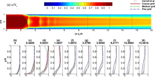
sup-port this statement figures 7 to 11 compare profiles of streamwise velocity, turbulent kinetic energy, and Reynolds stresses between the CFD results
be-tween the three grids and experiments. From figure 8 growth of turbulent kinetic energy, k, downstream of the first shock is observed. As the k-ω SST
model is used in its simplest formulation, it does not include a limiter for k, therefore the growth of k downstream of the shock is expected. No
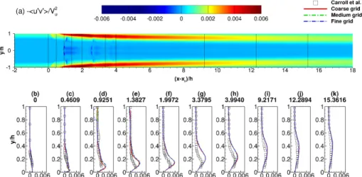
signifi-cant differences in the Reynolds stress profiles between the medium and fine grids were observed. The < u0u0 > /V2
u Reynolds stress is underpredicted throughout the beginning of the interaction whereas the−< u0v0 > /Vu2 and
< v0v0 > /V2
u components are overpredicted throughout the entire interac-tion. As a result, the turbulent kinetic energy is also overpredicted. However, the good agreement between the medium and fine grids in the Reynolds stress
profiles also suggests that the solution is grid converged. To further support the grid convergence, a grid convergence index (GCI) is calculated based on
the number of grid points N and the location of the start of the interaction
xr listed in table 2. For the calculation of the GCI, the method of Roache
[31] is used, which takes into account non-equal grid refinement ratios and requires at least three-grids (two levels of refinement). Table 5 shows the grid
sizes and refinement ratios and table 6 the calculated order of convergence, the asymptotic solution for xr, and the grid convergence index reported on
Figure 4: Wall pressure (a) and Mach number contours for the coarse (b), medium (c), and fine (d) grids
the finer grids. The value in the last column of table 6 shows that the
solu-tions obtained on the coarse, medium, and fine grids are in the asymptotic range of convergence, further supporting the statement that the solution is
grid converged. Despite the satisfactory grid convergence as seen from figure 4 the wall pressure is still slightly overpredicted.
Table 5: Grid sizes and refinement ratios for the coarse, medium, and fine grids Grid Grid sizeh Refinement ratior xr
Fine (1) 1.0000 1.7623 27.7206 Medium (2) 1.7623 1.6793 27.5227 Coarse (3) 2.9594 - 26.6968
Figure 5: Centreline Mach number for the coarse, medium, and fine grids
Figure 6: Skin friction coefficient for the coarse, medium, and fine grids
Figure 7: Streamwise velocity contoursu/Vufor the fine grid (a) and profiles (b-k) for the
coarse, medium, and fine grids
Table 6: Order of convergence, asymptotic solution and grid convergence index calculated from the coarse, medium, and fine grids
Order of convergencep Asymptotic solution forxr GCI23% GCI12% rpGCI12/GCI23
Figure 8: Turbulent kinetic energy k/V2
u for the fine grid (a) and profiles (b-k) for the
coarse, medium, and fine grids
Figure 9: Reynolds stress contours < u0u0 > /Vu2 for the fine grid (a) and profiles (b-k) for the coarse, medium, and fine grids
Figure 10: Reynolds stress contours−< u0v0> /V2
u for the fine grid (a) and profiles (b-k)
for the coarse, medium, and fine grids
Figure 11: Reynolds stress contours < v0v0 > /Vu2 for the fine grid (a) and profiles (b-k) for the coarse, medium, and fine grids
Figure 12: Wall pressure (a) and Mach number contours for the k-ω(b), baseline k-ω (c), k-ω SST (d), and k-ω EARSM (e) turbulence models on the fine grid
4.1.2. Turbulence modelling
Following the grid refinement study, a study on turbulence models was performed on the fine grid. The standard k-ω [26], baseline k-ω [26], and
k-ω EARSM [27, 28] turbulence models were used. Figure 12 shows the wall pressure and Mach number contours. Substantial variation of the location
of the first shock wave is observed depending on the turbulence model used. The k-ω EARSM model predicts the shock at the most upstream location
whereas the baseline k-ω at the most downstream location. The difference is ∆x/h≈6.2882 (13.67 % of the domain length). The shortest shock train is
predicted by the k-ω model whereas the longest by the k-ω EARSM model.
Differences in the Mach stem height are most likely due to the separation sizes. For the k-ω EARSM model the height of the separation (line where
u/Vu =−1×10⁻³) is y/h= 0.05437 whereas for the baseline k-ω it isy/h= 0.01883. The differences in the shock train length and location between
the turbulence models are expected as each turbulence model develops the boundary layer differently for fixed inlet-outlet boundary conditions.
4.2. Three-dimensional results
4.2.1. Symmetry boundary conditions
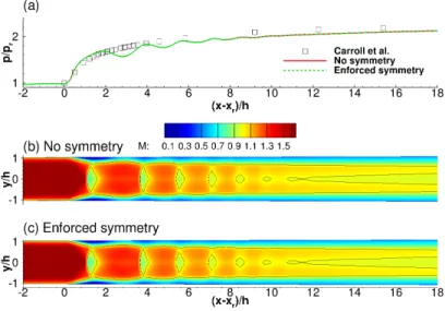
No differences in the wall pressure and Mach number contours are ob-served between the simulations on the full and the quarter domain with
enforced symmetries. Figure 13 shows the wall pressure and Mach number contours for both grids obtained with the k-ω SST model. The solid black
line indicates a Mach number of M = 1. The initial pressure rise occurs at the same position independent of the symmetry boundary conditions.
Simi-lar observations were made for the k-ωEARSM turbulence model on the fine grid with and without symmetry. It can be concluded that the wall pressure
Figure 13: Wall pressure (a) and Mach number contours for the extra coarse grid with (c) and without (b) symmetry boundary conditions
4.2.2. Grid refinement
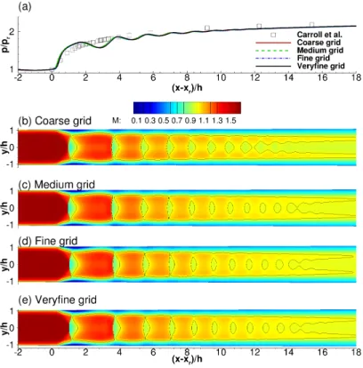
The wall pressure distribution p/pr for the stepwise increased resolution in the x- direction is shown in figure 14 (a). The solid line corresponds to
the coarse grid, the dashed line to the medium grid, and the dash-dotted line to the fine grid. Figure 14 also shows the Mach number contours of
the pseudo-shock system at the x-y symmetry plane. The solid black line indicates a Mach number of M = 1. No significant changes in the shape
of the pseudo-shock system are observed as the grid is refined. The wall pressure and the centreline Mach number, shown in figure 15 for the coarse,
medium, fine, and veryfine grids are practically identical showing that the medium grid is adequate for capturing the flow features. In addition, figures
16 and 17 show the wall pressure and the centreline Mach number for the medium and fine grids obtained with the k-ω EARSM turbulence model.
Figure 14: Wall pressure (a) and Mach number contours for the coarse (b), medium (c), fine (d), and veryfine (e) grids obtained with the k-ω SST turbulence model
Again, no differences in the wall pressure and centreline Mach number were observed suggesting that the medium grid should be used for further
Figure 15: Centreline Mach number for the coarse, medium, fine, and veryfine grids ob-tained with the k-ωSST turbulence model
Figure 16: Wall pressure for the medium and fine grids obtained with the k-ω EARSM turbulence model
Figure 17: Centreline Mach number for the medium and fine grids obtained with the k-ω EARSM turbulence model
4.2.3. Turbulence modelling
Several turbulence models and their effect on the sensitivity of the solution
are investigated. In particular, the turbulence models considered are the eddy-viscosity based - standard k-ω [26], baseline k−ω [26], and k-ω SST [26] models and the Reynolds stress based - the k-ω EARSM [27, 28] model. Figure 18 shows the wall pressure and the Mach number distribution for all
models. The standard k-ωturbulence model predicts the shortest shock train with 4 shocks following the initial normal shock. The baseline k-ω and the
k-ω SST turbulence models predict longer shock trains with the k-ω SST predicting the longest shock train from all models. This behaviour is similar,
but not identical, to two-dimensional simulations. All linear eddy-viscosity based models (EVMs) - the standard k-ω, baseline k-ω, and the k-ω SST
predict a wall pressure featuring small oscillations due to the strong shocks and large corner vortices. From the solid black line which indicates the sonic
condition, M = 1, it is seen that the EVMs predict the supersonic core flow to be much closer to the wall, due to the missing separation at the upper
and lower walls. The Reynolds stress based k-ωEARSM model, on the other hand, predicts separation at the upper and lower walls and shows no pressure
oscillations on the wall. From the Mach number contours, it can be seen that the supersonic core flow is not as close to the wall as the one predicted by the
EVMs. Figure 23 shows that the boundary layer predicted by the k-ωSST is less prone to separation resulting in stronger pressure oscillations where the
shocks are formed. The k-ω EARSM model underpredicts the wall pressure, due to the overprediction of the separation at the upper and lower walls as
Figure 18: Wall pressure (a) and Mach number contours for the standard k-ω(b), baseline k-ω (c), k-ω SST (d), and k-ω EARSM (e) turbulence models
the best agreement with the experiments.
Figure 19 shows the three-dimensional structure of the pseudo-shock sys-tem. The M = 1 iso-surface visualizes the structure of the shock train and
the following mixing zone. The u/Vu =−1×10⁻³ iso-surface visualises the separation zones. For the EVMs the dominating phenomenon is a large
cor-ner separation and no or little separation at the centreline. The shape of the shock train and the following mixing region is octagonal. In contrast,
the EARSM model shows little corner separation due to its suppression by the secondary (corner) flows. Larger separation is observed at the upper and
lower walls and the shape of the pseudo-shock system is more rectangular than octagonal. The separation at the centreline also affects the initial shock
structure. Although the EARSM model is in good agreement with experi-ments in terms of wall pressure, it predicts a larger centreline Mach number downstream of the initial shock. This further shows the importance of cap-turing both the corner and centreline separations accurately as they affect the initial shock structure. Figure 20 shows the visualization of the wall shear stress using friction lines just above the wall for each turbulence model
and figure 21 compares the visualization of the k-ωEARSM wall shear stress using friction lines just above the wall to the oil flow visualization from the
experiment. Red lines indicate flow features such as the centreline separation and the corner flows. Apart from the large separation at the centreline
pre-dicted by the model, it appears to capture well the flow structure near the corners. In addition to the comparison of the three-dimensional structure
of the pseudo-shock system, figures 24 to 29 compare streamwise velocity, wall-normal velocity, turbulent kinetic energy, and Reynolds stress profiles
Figure 19: M = 1 (shaded green) andu/Vu=−1×10−3 (shaded blue) isosurfaces for the
standard k-ω(a), baseline k-ω (b), k-ω SST (c), and k-ω EARSM (d) turbulence models
at several stations with the experiment for the different eddy-viscosity and Reynolds stress turbulence models. These quantities, especially the Reynolds
stresses are rarely compared as they are often not measured in MSWBLI experiments. Since in the MSWBLI experiment by Carroll et al. [3] the
< u0u0 > /Vu2, − < u0v0 > /Vu2, and < v0v0 > /Vu2 Reynolds stress com-ponents were measured they will be the ones compared to the simulations.
Figure 25 shows the wall-normal velocity profiles and contours. As the cen-treline Mach number, the differences in the profiles between the EVMs and EARSM are attributed to the initial shock structure. From the Reynolds stress profiles, it is seen that the EVMs and the EARSM underpredict the
< u0u0 > /Vu2 Reynolds stress component throughout the beginning of the interaction. The< v0v0 > /Vu component is overpredicted throughout the
en-tire interaction by all models, with the k-ω EARSM model giving the largest overprediction.
Figure 20: Visualization of the wall shear stress using friction lines just above the wall for the k-ω (a), baseline k-ω (b), k-ω SST (c), and k-ωEARSM (d) turbulence models
Figure 21: Comparison of the visualization of the k-ω EARSM wall shear stress using friction lines just above the wall (top) with the oil flow visualization from the experiment (bottom)
Figure 22: Centreline mach number for the standard k-ω, baseline k-ω, k-ωSST, and k-ω EARSM turbulence models
Figure 23: Skin friction for the k-ωSST and the k-ω EARSM turbulence models
Figure 24: Streamwise velocity u/Vu contours (a) for the k-ω EARSM and profiles (b-k)
for the standard k-ω, baseline k-ω, k-ω SST, and the k-ω EARSM turbulence models on the medium grid
Figure 25: Wall normal velocity v/Vucontours (a) for the k-ω EARSM and profiles (b-k)
for the standard k-ω, baseline k-ω, k-ω SST, and the k-ω EARSM turbulence models on the medium grid
Figure 26: Turbulent kinetic energy k/V2
u contours (a) for the k-ω EARSM and profiles
(b-k) for the standard k-ω, baseline k-ω, k-ωSST, and the k-ωEARSM turbulence models on the medium grid
Figure 27: Reynolds stress < u0u0 > /V2
u contours (a) for the k-ω EARSM and profiles
(b-k) for the standard k-ω, baseline k-ω, k-ωSST, and the k-ωEARSM turbulence models on the medium grid
Figure 28: Reynolds stress−< u0v0 > /V2
u contours (a) for the k-ω EARSM and profiles
(b-k) for the standard k-ω, baseline k-ω, k-ωSST, and the k-ωEARSM turbulence models on the medium grid
Figure 29: Reynolds stress< v0v0 > /V2
u contours (a) and profiles (b-k) for the standard
k-ω, baseline k-ω, k-ω SST, and the k-ω EARSM
with two- and three-dimensional scale-resolving (LES) simulations from Mor-gan et al. [15, 16] and Roussel et al. [18].
Figure 30: Comparison of the wall pressure from the k-ω EARSM simulation to other scale-resolving simulations of the same experiment
As the scale resolving simulations are performed at a Reynolds number a magnitude lower than the experiment Reδr = 16200 the shock train is
expected to be located farther downstream than in the experiment. Fur-thermore, it should be expected that confinement effects cannot be matched
Figure 31: Isosurfaces of the second invariant of the velocity gradient tensor Q = 0.01 colored by Mach number and countours of the density gradient magnitude in grayscale (numerical schlieren) of the DES (DES 97) (k-ω SST) simulation. The synhtetic eddy method by Jarrin et al. [32] was used at the inflow.
at every location in the flow. The scale resolving simulations predict bet-ter the initial pressure rise, however, the downstream pressure rise is
sig-nificantly underpredicted. The underprediction may be attributed to the different boundary layer growth due to the lower Reynolds number of the
simulations or to the requirement for lower backpressure for a stable pseudo-shock system (Morgan et al. [16]). A DES (DES 97) (k-ω SST) with a
SEM inflow by Jarrin et al. [32], shown in figure 31, performed on a short domain also underpredicted the wall pressure. The k-ω EARSM turbulence
model used here captures well the pressure upstream and downstream of the shock train. A distinct ”plateau” in the wall pressure is observed after the
initial pressure rise which is attributed to the separation predicted at the
centreline. Despite the underprediction of the wall pressure due to the cen-treline separation the k-ω EARSM model shows satisfactory agreement with
the experimental results at a fraction of the computational cost required for
scale-resolving methods.
4.3. Three-dimensional results for Sun et al. test case
In addition to the MSWBLI case of Carroll et al. [3] complimentary
simulations were performed for the MSWBLI case of Sun et al. [8] and the MSWBLI case of Fi´evet et al. [10]. The k-ω EARSM turbulence model
was used for both cases and the grids considered were of sufficient length to allow the boundary layer to develop since it showed the best agreement
with experiments for the case of Carroll et al. [3]. Further adjustments to the Mach number at the inlet and the pressure at the outlet were made to
match the experimental conditions as close as possible. This section outlines the results for the MSWBLI case of Sun et al. [8]. The Mach number and
Reynolds number for the case areMr= 2.0 andReh = 1×10⁶. The numerical setup for the simulations is shown in figure 32. The simulation parameters
are listed in table 7.
Iu,Mu,pu,δu Flow p Mr, δr,pr 1840mm x y 80.00 mm (2h) xr xu
Figure 32: Sketch of the numerical setup of the MSWBLI experiment by Sun et al. [8]
Three two-dimensional grids were used for a grid convergence study and one three-dimensional for the quantification of the spanwise effects introduced
by the flow confinement. Figure 33 shows the wall pressure and the Mach number contours for the k-ω SST turbulence model on the coarse, medium,
and fine grids. As the grid is refined no differences in the wall pressure are
ob-served. Even the extra coarse grid is capable of resolving the pressure across the MSWBLI adequately. Figure 34 shows the wall pressure for the medium
grid (3D) obtained with the k-ω EARSM turbulence model. Similarly to the MSWBLI results for the case of Carroll et al. [3], the wall pressure is
underpredicted downstream of the first shock, however, good predictions are observed upstream and downstream.
Figure 33: Wall pressure (a) and Mach number contours for the 2D coarse (b), 2D medium (c), and 2D fine (d) grids
Figure 35 shows the three-dimensional structure of the pseudo-shock
sys-tem. The M = 1 iso-surface visualizes the shock train and the following mixing zone. The u/Vu = −1×10⁻³ iso-surface visualizes the separation
Table 7: Two-and-three-dimensional RANS simulations parameters for the case of Sun et al. [8]
Grid Iu% Mu Mr δrmm δr/h xr/h p/pu p/pr Turbulence model Extra coarse (2D) 1.0 2.00 1.916 12.300 0.3075 21.2924 3.5991 3.1629 k-ωSST Coarse (2D) 1.0 2.00 1.911 12.380 0.3095 21.6732 3.5991 3.1896 k-ωSST Medium (2D) 1.0 2.00 1.916 12.616 0.3154 22.3024 3.5991 3.1723 k-ωSST Medium (3D) 1.0 2.15 1.998 10.196 0.2549 19.6059 4.2887 3.4552 k-ωEARSM Experiment [8] - - 2.000 10.000 0.2500 0 - 3.1549
Figure 34: Wall pressure (a) and Mach number contours for 3D medium grid (b)
due to their suppression by the secondary corner flows. Larger separations are observed on all four walls. The pseudo-shock shape is again more
rectan-gular than octagonal. The larger separations at the walls are again the cause for the underprediction of the wall pressure seen in figure 34.
4.4. Three-dimensional results for Fi´evet et al. test case
The last MSWBLI case considered for simulation is the MSWBLI case by
Fi´evet et al. [10]. The Mach number and Reynolds number for the case are
Mr = 2.0 andReh = 1.2370×10⁵. The numerical setup for the simulations is shown in figure 36. The simulation parameters are listed in table 8. Figures
Figure 35: M = 1 (shaded green) andu/Vu=−1×10−3 (shaded blue) isosurfaces for the
k-ω EARSM turbulence model on the medium grid (3D)
37 and 38 show the wall pressure, Mach number contours and centreline
pressure for the coarse and medium grids obtained with the k-ω EARSM turbulence model. Iu,Mu,pu,δu Flow p Mr, δr,pr 1710 mm x y 69.80 mm (2h) xr xu
Figure 36: Sketch of the numerical setup of the MSWBLI experiment by Fi´evet et al. [10]
The wall pressure predicted by the k-ω EARSM turbulence model is in good agreement with the wall pressure calculated from Fi´evet et al. [10]
and with the experimental results reported in the same paper. Similarly to the MSWBLI results for the case of Carroll et al. [3], the wall pressure is
underpredicted downstream of the first shock.
No experimental data for centreline Mach number or pressure is available,
Figure 37: Wall pressure (a) and Mach number contours for the coarse (b) and medium (c) grid obtained with the k-ω EARSM turbulence model
Table 8: Three-dimensional RANS simulations parameters for the case of Fi´evet et al. [10] Grid Iu% Mu Mr δrmm δr/h xr/h p/pu p/pr Turbulence model Coarse 1.0 2.210 2.035 8.8498 0.2536 14.3340 4.2394 3.1828 k-ωEARSM Medium 1.0 2.210 2.024 9.0007 0.2579 14.5315 4.2394 3.1904 k-ωEARSM Experiment [10] - - 2.000 9.8000 0.2800 0 - 3.1862
Figure 38: Centreline pressure for the coarse and medium grid obtained with the k-ω EARSM turbulence model
39 shows the three-dimensional structure of the pseudo-shock system. The
Theu/Vu =−1×10⁻³ iso-surface visualizes the separation zones. The corner separations predicted by the k-ω EARSM turbulence model are small due to their suppression by the secondary corner flows. Larger separations are
observed on all four walls. The pseudo-shock shape is again more rectangular than octagonal. The larger separations at the walls are again the cause for
the slight underprediction of the wall pressure seen in figure 37.
Figure 39: M = 1 (shaded green) andu/Vu=−1×10−3 (shaded blue) isosurfaces for the
k-ω EARSM turbulence model on the medium grid
Figure 40 compares the wall pressures from the experiments (Carroll et
al. [3]; Sun et al. [8]) and the numerical simulation of Fievet et al. [10] to the respective 3D solutions obtained with the k-ω EARSM model. The
simulations exhibit the same trends as the experiments, further supporting the consistency of the k-ω EARSM model across the three MSWBLI
inter-actions. The good agreement in wall pressure ahead and downstream of the MSWBLI interactions was accompanied by good agreement in the profiles
of streamwise velocity, wall-normal velocity, turbulent kinetic energy, and
Figure 40: Wall pressure of the cases of Carroll et al. [3], Sun et al. [8], and Fi´evet et al. [10] and corresponding 3D k-ω EARSM simulations
5. Conclusions and future work
A set of conclusions are drawn in this section along with some suggestions
for future work.
The use a long domain with a higher Mach number at the inlet, to account for blockage, allows a boundary layer to develop properly and the pre-shock Mach number to be matched.
Although two-dimensional simulations exhibit good agreement with ex-periments they should not be employed as they do not include spanwise effects.
The effect of corner separations on the centreline separation necessitates the inclusion of spanwise effects.
The flow was shown to exhibit symmetry, hence a quarter of the domain was simulated.
The eddy-viscosity based models considered -k−ω, baselinek−ω, andk−ω
SST overpredict the corner separations and underpredict the centreline separation. This leads to pressure oscillations at the wall not reported in the experiments.
The capability of the k−ω EARSM model to account for the secondary flows improves the wall pressure prediction. The model predicted smaller corner separations leading to a larger centreline separation in agreement with the experiment.
Across the three computed cases the k−ω EARSM displayed consistent prediction of the wall pressure.
Further computations with the k-ω EARSM model in a zonal approach, combined with a scale-resolving turbulence simulation method are also envisaged. Realistic intake geometries are also targeted including investi-gation of non-adiabatic wall conditions.
A parametric study covering the shock configuration and pressure recovery over a range of flow conditions is also underway
References
[1] K. Matsuo, M. Y., H.-D. Kim, Shock train and pseudo-shock phenomena
in internal gas flows, Progress in Aerospace Sciences 35 (1999) 33–100.
[2] B. Carroll, Numerical and experimental investigation of multiple shock wave/turbulent boundary layer interactions in a rectangular duct, Ph.D.
[3] B. Carroll, J. Dutton, An ldv investigation of a multiple normal shock
wave/turbulent boundary layer interaction, in: 27th Aerospace Sciences Meeting, 1989.
[4] B. Carroll, J. Dutton, Characteristics of multiple shock wave/turbulent boundary-layer interactions in rectangular ducts, Journal of Propulsion
and Power 8 (2) (1992) 441–448.
[5] B. Carroll, J. Dutton, Multiple normal shock wave/turbulent
boundary-layer interactions, Journal of Propulsion and Power 8 (2) (1992) 441–448.
[6] B. Carroll, J. Dutton, Multiple normal shock wave/turbulent
boundary-layer interactions, AIAA Journal 30 (1) (1992) 43–48.
[7] B. Carroll, P. Lopez-Fernandez, J. Dutton, Computations and experi-ments for a multiple normal shock/boundary-layer interaction, Journal
of Propulsion and Power 9 (3) (1993) 405–411.
[8] L. Sun, H. Sugiyama, M. K., T. Hiroshima, A. Tojo, Numerical and
experimental study of the mach 2 pseudo-shock wave in a supersonic duct.
[9] R. Fi´evet, H. Koo, V. Raman, A. Auslender, Numerical simulation of shock trains in a 3d channel, in: AIAA Science and Technology Forum
and Exposition, 2016.
[10] R. Fi´evet, H. Koo, V. Raman, A. Auslender, Numerical investigation of
shock-train response to inflow boundary-layer variations, AIAA Journal 55 (9) (2017) 2888–2900.
[11] R. Klomparens, J. Driscoll, M. Gamba, Unsteadiness characteristics and
pressure distribution of an oblique shock train, in: 53rd AIAA Aerospace Sciences Meeting, 2015.
[12] R. Klomparens, J. Driscoll, M. Gamba, Response of a shock train to
downstream back pressure forcing, in: 54th AIAA Aerospace Sciences Meeting, 2016.
[13] A. Weiss, A. Grzona, H. Olivier, Behavior of shock trains in a diverging duct, Shock Waves 49 (1) (2010) 297–306.
[14] T. Gawehn, A. G¨ulhan, N. S. Al-Hasan, G. H. Schnerr, Experimental
and numerical analysis of the structure of pseudo-shock systems in laval nozzles with parallel side walls, Shock Waves 20 (1) (2010) 297–306.
[15] B. Morgan, K. Duraisamy, L. S.K., Large-eddy and rans simulations of a
normal shock train in a constant-area isolator, in: 50th AIAA Aerospace Sciences Meeting including the New Horizons Forum and Aerospace
Ex-position, 2012.
[16] B. Morgan, J. Larsson, S. Kawai, L. S. K., Large-eddy simulations of a normal shock train in a constant-area isolator, AIAA Journal 52 (3)
(2014) 539–558.
[17] Z. Vane, I. Bermejo-Moreno, S. K. Lele, Simulations of a normal shock train in a constant area duct using wall-modelled les, in: 43rd Fluid
Dynamics Conference, 2013.
m=1.61, in: 22nd AIAA Computational Fluid Dynamics Conference,
2015.
[19] R. Steijl, G. N. Barakos, K. Badcock, A framework for cfd analysis of
helicopter rotors in hover and forward flight, International Journal for Numerical Methods in Fluids 51 (8) (2006) 819–847.
[20] R. Steijl, G. N. Barakos, Sliding mesh algorithm for cfd analysis of heli-copter rotor-fuselage aerodynamics, International Journal for Numerical
Methods in Fluids 58 (5) (2008) 527–549.
[21] S. Osher, S. Chakravarthy, Upwind schemes and boundary conditions
with applications to euler equations in general geometries, Journal of Computational Physics 50 (3) (1983) 447–481.
[22] B. van Leer, Towards the ultimate conservative difference scheme. v.
a second-order sequel to godunov’s method, Journal of Computational
Physics 32 (1) (1979) 101–136.
[23] G. D. van Albada, B. van Leer, W. W. Roberts, A comparative study of computational methods in cosmic gas dynamics, Astronomy and
As-trophysics 108 (1) (1982) 76–84.
[24] O. Axelsson, Iterative Solution Methods, Cambridge University Press,
1994.
[25] D. Wilcox, Reassessment of the scale-determining equation for advanced
[26] F. Menter, Two-equation eddy-viscosity turbulence models for
engineer-ing applications, AIAA Journal 32 (8) (1993) 1598–1605.
[27] S. Wallin, A. Johansson, An explicit algebraic reynolds stress model
for incompressible and compressible turbulent flows, Journal of Fluid Mechanics 403 (2000) 89–132.
[28] A. Hellsten, New advanced k-omega turbulence model for high-lift aero-dynamics, AIAA Journal 43 (9) (2005) 1857–1869.
[29] B. Morgan, Large-eddy simulation of shock/turbulence interactions in hypersonic vehicle isolator systems, Ph.D. thesis, Stanford University
(2012).
[30] T. Handa, M. Masuda, Three-dimensional normal shock-wave/boundary-layer interaction in a rectangular duct, AIAA Journal
43 (10) (2005) 2182–2187.
[31] P. J. Roache, Perspective: A method for uniform reporting of grid
re-finement studies, Journal of Fluids Engineering 116 (3) (1994) 405–413.
[32] N. Jarrin, D. Laurance, S. Benhamadouche, R. Prosser, A
synthetic-eddy-method for generating inflow conditions for large eddy simulation, International Journal of Heat and Fluid Flow 27 (4) (2006) 585–593.
Nomenclature
(.)0 Fluctuation component of a quantity
(.)u Quantity at inlet
<(.)> Reynolds averaged quantity
δ Boundary layer thickness
δ/h Ratio of boundary layer thickness to duct half height (confine-ment ratio)
δ∗ Boundary layer displacement thickness
µ Molecular viscosity
µt Eddy viscosity
ω Specific dissipation rate
θ Boundary layer momentum thickness
h Duct half-height
I Turbulence intensity
k Turbulent kinetic energy
p Static pressure
r Refinement ratio
Reδ Reynolds number based on boundary layer thickness
Reh Reynolds number based on the duct half-height
v Wall normal velocity component
w Spanwise velocity component
x Streamwise coordinate
y Wall normal coordinate
z Spanwise coordinate
BSL Baseline
DES Detached Eddy Simulation
EARSM Explicit Algebraic Reynolds Stress Model
GCI Grid Convergence Index
LES Large Eddy Simulation
MSWBLI Multiple Shock Wave Boundary Layer Interaction
SEM Synthetic Eddy Method