Multiscale Network Analysis for Financial Contagion

(1)

Kent Academic Repository

Full text document (pdf)

Copyright & reuse

Content in the Kent Academic Repository is made available for research purposes. Unless otherwise stated all content is protected by copyright and in the absence of an open licence (eg Creative Commons), permissions for further reuse of content should be sought from the publisher, author or other copyright holder.

Versions of research

The version in the Kent Academic Repository may differ from the final published version.

Users are advised to check http://kar.kent.ac.uk for the status of the paper. Users should always cite the published version of record.

Enquiries

For any further enquiries regarding the licence status of this document, please contact:

[email protected]

If you believe this document infringes copyright then please contact the KAR admin team with the take-down information provided at http://kar.kent.ac.uk/contact.html

Citation for published version

Alexandridis, Antonios and Ladas, Anestis (2019) Multiscale Network Analysis for Financial Contagion. In: 9th International Conference of the Financial Engineering and Banking Society, 30 May - 1 Jun 2019, Prague, Czechia. (In press)

DOI

Link to record in KAR

https://kar.kent.ac.uk/74566/

Document Version

(2)

Multiscale Network Analysis for

Financial Contagion

Antonios K. Alexandridis1

Anestis C. Ladas2

Wednesday, May 8, 2019

Abstract: Contagion in financial markets has been one the most active areas of research, especially during the last decade and due to the major incidents during the Global Financial Crisis and the European Financial Crisis. However, two of the most important questions that remain after a financial crisis are what are the determinants of the crisis and how can we forecast an incident based on suitable indicators. The purpose of this study is twofold. First, to develop a measure of contagion based on the multiscale nature of the financial contagion. Second, to examine how financial contagion is spread in the US economy in different frequencies based on the proposed measure. We assert that important information on an upcoming crisis, not observed in the original data, may be revealed by performing a time-frequency analysis of the time-series and the cross-section of stock returns. We use wavelet analysis to decompose the returns and network analysis to compute various network characteristics related to contagion. Our proposed methodology allow us to: understand the short-, mid- and long-term connections of the network, bring out structures/relations that are not visible initially and mask the true connections between companies, study how the networks measures change over scale, and finally, examine the distribution of contagion at different time-horizons and scales.

Keywords: contagion, wavelet analysis, network analysis

1_{Corresponding author, Antonis Alexandridis, Kent Business School, University of Kent, Canterbury, Kent,}

CT2 7PE, UK, email: [email protected]

2_{Department of Accounting and Finance, School of Business Administration, University of Macedonia,}

(3)

1. Introduction

Contagion in financial markets has been one of the most active areas of research especially during the last decade and the major incidents during the global financial crisis and the European financial crisis. Most of this research aims at uncovering the factors that affect contagion in order to propose solutions that limit it in the future. One of the factors that impose burdens in this task is the structure of the financial market itself. The rapid development of financial markets through the last decades led them to evolve in complex systems due to the large number of agents and relations among them. These complex structures increase the difficulty of the assessment of contagion. In this respect, thinking of financial markets as complex systems, it is natural to use methods like network analysis in order to assess the relationships between the various agents, (for example see Mantegna (1999). Previous studies have used a number of methods to assess contagion among which were connectedness measures (Billio et al. (2012).

One of the important steps in the analysis is to correctly identify the relations between the actors of the network. Previous studies were based on stock returns to form either undirected networks, with the use of correlations, or directed networks with the use of Granger causality tests (Billio et al. (2012). In both of these cases a typical problem that emerges, taking in mind the large number of relations, is that information may continue to be hidden due to the large complexity of the network especially in the case of daily data. In this respect, Onnela et al.

(2004) used a Minimum Spanning Tree algorithm to filter the relations and extract from the network those relations that were deemed important for their analysis. However, such methods do not come without costs. The algorithm used in such cases may neglect essential information from the network (Chi et al., 2010).

In this study, we focus on the multiscale analysis of financial contagion based in the application of wavelet analysis (WA). For a correct analysis of daily returns, both local and global information is needed. Hence, WA is ideal for this task since it can reveal these characteristics by decomposing the stock returns time-series in different scales. Moreover, the wavelet transform has good frequency resolution for low-frequency events and good time resolution for high-frequency events and can bring out trends, jumps or structural breaks, Mallat (1999).

Following Billio et al. (2012), we estimate the adjacency matrix of the network on the wavelet decomposed data using Granger causality tests and then we compute a number of network characteristics related to contagion. In turn, these measures are used as determinants

(4)

of contagion, where contagion is estimated as the out-degree centrality of a node. Put differently, a node with a high number of out-connections has a higher likelihood to transfer contagion to the nodes in his neighbor.

The research motivation of the study lies with previous studies that tried to assess contagion in financial systems that are complex systems with large numbers of actors. In these cases, the frequency of the data may impose additional limitations to the analysis. The present study attempts to develop a method for assessing the relation in a network by first decomposing the data used to assess the relation (stock returns) based on both its frequency and time domain. For the task in hand, we use wavelet analysis to disentangle the various signals that may lie in the time series and the cross-section of stock returns and then use these wavelet transforms to form the network and calculate the network characteristics.

The research question of the study concerns the likely existence of differences in the relation between contagion and network characteristics, due to the use of signals related to different measurement frequencies retrieved from the primary data, to estimate the variables of interest (contagion and network variables). In other words, specific contagion incidents of interest may take place at different frequencies than the frequency observed in the original data. Thus, the merit of this analysis has to do with the decomposition of stock returns in various frequencies prior to estimating the network and contagion variables. This approach enables us to examine both the relationship between contagion and network characteristics, as well as, the changes in this relation as we move from higher to lower frequencies. WA is ideal for this type of analysis since it alleviates the problem of data reduction when different frequencies are used.

The results of the study show that the decomposition provides a number of important research findings that could not be uncovered using only the raw data. In this respect, certain network characteristics like clustering may enhance the contagion effects in some cases, while eigenvector centrality seems to limit it, but the effects of both clustering and eigenvector centrality are not constant at different scales. Moreover, contagion seems to be limited in certain cases by the contemporaneous presence of clustering and eigenvector centrality. In sum our results point towards the existence of different information content for contagion through the various timescales.

The remainder of the study is as follows: Section 2 reviews the literature and develops the research hypotheses. Section 3 explains the methodology used in the study. Section 4 presents the descriptive statistics and analyses the empirical results and last Section 7 concludes the study.

(5)

2. Literature Review and Research Hypotheses

Explaining contagion has been the subject of a large number of studies due to the profoundly negative effects that it can have in the financial markets and the economy in general. Studies on contagion used a number of methods which likely suffered from loss of information due to the complex nature of the financial system. During the last years a new trend arose based on the use of networks. Mantegna (1999) is one of the first studies to use network models in order to examine the relation in the stock market. Billio et al. (2012) use a number of connectedness measures as proxies for systemic risk. Elliott et al. (2014) use network analysis to directly examine the impact of contagion in a financial network among intermediaries. Acemoglu et al.

(2015) develop a methodology for examining contagion based on the use of financial networks. A problem that emerges in the empirical application of the networks is the large information set that may emerge and makes inference difficult. Some studies apply filters that eliminate part of the information in the network in order to provide a clearer view of the relation between the actors if the network, i.e. Tumminello et al. (2005). In this strand of literature, Onnela et al. (2004) use a Minimum Spanning Tree algorithm which filters relations and extracts only those that are deemed important for the analysis. On the other hand, Chi et al. (2010) base the mapping of the relations on correlations and choose only correlation of high values in order to proceed to their analysis. However, using a subgraph of the total network in order to remove noise may lead to a loss of information.

Apart from filtering the relations in the network there are other tools that can be used to filter the noise and provide a more analytical view of large networks with a large number of nodes. In specific, partitioning based on the frequency of stock returns, by using WA, has provided a very powerful tool for decomposing time series. For example Kim & In (2005) use multiscale analysis to assess the relation between stock returns and inflation for a number of time scales. Reboredo & Rivera-Castro (2014) use a similar methodology based on WA to examine the relation between oil prices and stock returns. The authors argue that the main problem of the analysis on the above relation has to do with the limited time scales used, which can be encountered using a multiscale analysis.

Contagion in financial markets may follow a number of streams among which may be channels with short or medium-term dynamics. Put differently, contagion is like an epidemic, where the spread may not be observed only in the short term or only in the medium term. Therefore, allowing for a multiscale horizon may provide useful evidence on the spread of contagion that were previously unused due to focusing only on short term dynamics. Indeed,

(6)

Gençay et al. (2005) provide evidence that the relation between stock returns and beta becomes stronger as we move to higher scales.

Therefore, the research hypotheses of the study are related to differences in contagion between the timescales. In specific, the first set of research hypotheses assert that the degree of clustering is positively related to the outdegree centrality and moreover this relation becomes stronger as we move to higher scales (low frequency). The rational is that, the more closely related are the nodes the higher the likelihood of a high outdegree centrality due to the more probable spillover of shocks. Moreover, for low scale shocks, market mechanisms may be adequate to absorb it, however, for more persistent idiosyncratic shocks the contagion is more probable and is also a function of the connectedness. Therefore, the first set of research hypotheses of the study is formulated as follows:

H1A: The higher the connectedness of a bank in the form of clustering, the higher the number

of connections to other nodes in the form of outdegree centrality.

and

H1B: The relation between connectedness of a bank in the form of clustering and the number

of connections in the form of outdegree centrality is a direct function of the scale of the channel of contagion after a shock.

On the other hand, we expect that a shock for banks with high eigenvector centrality, which accounts for the importance of the other nodes to which the node of interest is attached, will be negatively related to contagion and this negative relation will become stronger as we move to higher scales. This hypothesis is based on the assertion that a shock in these firms may not pass through to their connected nodes if the later are significant nodes of the network and this effect will be a direct function of the size of scale. Put differently, the higher the scale the more immune are significant nodes of the network to contagion from less important nodes due to the existence of a larger time-window to attain the effects of the shock. Therefore, our second set of research hypotheses are as follows:

H2A: The higher the eigenvector centrality of a bank, the lower the number of connections

(7)

and

H2B: The relation between eigenvector centrality of a bank and the number of connections

in the form of outdegree centrality is an indirect function of the scale of the channel of contagion after a shock.

The third set of research hypotheses has to do with the contemporaneous effects of clustering and eigenvector centrality. In specific, we argue that any increasing effects of clustering on outdegree centrality may be limited by the contemporaneous presence of high eigenvector centrality. In this respect the third set of research hypotheses is as follows:

H3A The higher the eigenvector centrality and clustering the lower the probability of

contagion

and

H3B The higher the eigenvector centrality and clustering in higher scales the lower the

probability of contagion than in lower scales

The last research hypothesis has to do with the financial health of the firm. To assess the financial health of the firm we use accounting measures such as the book-to-market ratio, the leverage and the return-on-assets. We hypothesize that a bank with strong financial health, as measured by the previous indicators, will be more immune to contagion at least for lower scales. However, we expect that a prolonged period of shocks will likely lead to a generalized contagion in the market. Therefore, our third research hypothesis is as follows:

H4: High scale contagion is related positively to more financially healthy firms.

3. Research Methodology

The methodology of the study is divided in three interrelated parts. The first describes the use of wavelet analysis in the decomposition of stock returns based on scale. In the second part, we develop the financial network formation and the estimation of the network parameters. Finally, in the third part present the main models of this study.

(8)

3.1 Wavelet Analysis

In this section, we provide a quick presentation of the multiscale wavelet analysis (WA). The wavelet transform is localized in both time and frequency and overcomes the fixed time-frequency partitioning providing many advantages over alternative methods, e.g. (short-time) Fourier transform. The discrete wavelet transform provides efficient means of analyzing a time-series according to scales. WA is very flexible in handling very irregular data time-series and can be used to identify trends, jumps or periodicities that originally cannot be observed, Donoho & Johnstone (1994). As mentioned in Conlon et al. (2016), Ramsey (1999), these characteristics are very common in financial time-series. 3 Finally, using WA we can represent highly complex structures without knowing the underlying functional form which is of great benefit in economic and financial research, Ramsey (1999). In this study we use the Maximal Overlap Discrete Wavelet Transformation (MODWT) motivated by its many advantages over the classic DWT (see Percival & Walden (2000)).

The wavelet representation of a time-series is given by:

 

, , , , 1, 1, 1, ,

( ) _{j k} _{J k} _{J k} _{J k} _J _k _J _k _k _{j k}

k k k k

f t 



s  t 



d  t 



d _  _ t  



d  t (1)

where J is the number of scales and k is the kth_{coefficient. The smooth and detail component} coefficients are given by

 

, , , , j k j k s f t  t dt k j   



 (2)

 

, , , , j k j k d f t  t dt k j   



 (3)

respectively where the functions _{j k}_,

 

t and _{j k}_,

 

t are called the father and the mother wavelet functions. By setting

, , ( ) ( ) j j k j k k S t 



s t  (4) , , ( ) ( ) j j k j k k D t 



d t (5)

3_{A sample of recent papers that have used WA to analyse financial time-series can be found in Alexandridis}

& Zapranis (2013), (2014), Conlon & Cotter (2012), Conlon et al. (2016), Fernandez (2006), Gençay et al. (2005), In & Kim (2006), Kim & In (2005), Ramsey (1999).

(9)

the original time-series can be reconstructed. This reconstruction in called the multi-resolution analysis (MRA) and can be written as:

 

, , , , 1 1 ( ) _{J k} _{J k} _{j k} _{j k} _J( ) _J( ) _J ( ) ( ) k Z j Z k Z f t s  t d  t S t D t D _ t D t    







     (6)

At each level j of the MODWT we split the time series (the approximation S_j_₁) into two parts. This first one is a detail signal at level j, D_j, that captures short-term deviations in the

time-series while the second one is the new approximation at level j, S_j, that captures the long-term

components. We denote the original time-series as the approximation S₀.

3.2 Formation of the Network and Estimation of the Basic Parameters

We decompose the idiosyncratic returns to J+1 signals (D₁,...,D S_J, _J) obtained from the MODWT described in the previous section. Then we form the adjacency matrix of the network for each scale.

For the estimation of the idiosyncratic returns we use the CAPM with leads and lags of the market return, r_m, following Dimson (1979). The model is as follows:

  _  _   _  _ 

      

, 0 1 , 2 2 , 1 3 , 4 , 1 5 , 2 ,

i w m w m w m w m w m w i w

r r r r r r (7)

where ri,w is the weekly stock return of firm i at week w, rm is the market return and _{i w}_, is the error term. We estimate model (7) annually for each scale j.

The adjacency matrix, A, maps the relations between the nodes of the network into 1 and 0. It is a square matrix and is used to represent a graph through assigning 1 if there is a relation between nodes i and j and zero otherwise. If the graph is undirected (causality runs in both directions and is amphidromous) then the matrix is symmetric and the element i,j is equal to the element j,i. If the graph is a directed graph (the causality may run from one node to the other but the opposite is not compulsory) then the i,j element may not be equal to the j,i element of the matrix.

Following Billio et al. (2012), we perform Granger causality tests, Granger (1969), in order to map the network. Hence, we construct a directed network. Specifically, if the weekly returns

(10)

of firm i in week w Granger-cause the weekly returns of firm j in week w then the i,j element of the th

k adjacency matrix, corresponding to the th

k scale, takes the value of 1 and the value of 0 in the opposite case.

The adjacency matrix is used to estimate the out-degree of each node. The out-degree of node i, d_iout, is estimated as the number of other nodes that are affected by the node of interest.

We divide d_iout by the total number of nodes that could have been affected by the node of interest in order to standardize the measure as a percentage. As explained above, node i is affected by node j if the stock returns of the later Granger-cause the stock returns of the former. The total degree of node i is given by the summation of the in- and the out-degree,

tot in out

i i i

d d d .

We also compute the clustering coefficient between the nodes of the system following Fagiolo (2007). The methodology of Fagiolo is based on the methodology of Watts & Strogatz (1998) with the difference that is suited for binary directed networks:









3 2 1 2 T ii i _tot _tot i A A Clustering d d d         (8)

where A is the adjacency matrix,



T



3 ii

AA is the ii element of



A A T



3, dtot is the total degree and d_i is the number of bilateral edges between node i and its neighbors given that no

self-interactions exist, _i _ij _ji _ii2 i j

d a a A







 where A_ii2 is the i diagonal element of A2  A A. The last measure is the eigenvector centrality which measures the “prestige” of node i. High eigenvector centrality indicates that node i (or bank i) is highly connected or is connected to important neighbours (or both). Newman (2010) argues that estimating eigenvector centrality using a directed network may be problematic. To alleviate this we estimate the eigenvector centrality by constructing the adjacency matrix B based on the correlation matrix that uses as inputs the idiosyncratic stock returns. The eigenvector centrality measure is given by:



1



i ij j

j

Eigencentrality B Eigencentrality (9)

where λ is a the leading eigenvalue of the adjacency matrix B.

We estimate the above measures for each scale of the decomposed returns.

(11)

3.3 The Main Models

The contagion measure used in the study is based on financial networks contagion studies (i.e. Billio et al., 2012). We define contagion as the transmission of shocks among the connected firms. In this respect, we measure connectedness using the out-degree centrality. Out-degree centrality is a measure of connections of the node of interest to others. A high out-degree centrality expresses the risk a specific bank related to its shocks flowing through the network. Hence, a high number of nodes affected by the node of interest leads to a higher likelihood of contagion. For the task in hand we use the decomposition methodology described in Section 3.1 and estimate the out-degree centrality for the J+1 decompositions of the idiosyncratic returns. Next, we use Granger Causality tests and estimate the contagion variable as the ratio of the number of nodes affected by the node of interest to the total number of nodes that could have been affected by the node of interest and this variable is estimated for each J+1

decomposition. The main model express contagion as a function of a number of accounting and auditing characteristics of a bank and is estimated in an under a panel data approach with period fixed effects and robust standard errors. In algebraic form the model is as follows:

                  , 0 1 , 2 , 3 , 4 , 5 , 5 , 6 , , i t i t i t i t i t i t i t i t i t

Contagion Size Leverage MtB

RoA NCSKEW Eigcentrality Clustering (10)

where Size is the logarithm of total assets, Leverage is the bank’s leverage ratio, MtB is the Market-to-Book ratio and RoA is the return on assets. Clustering is the measure of clustering given by equation (8), NCSKEW is the negative skewness stock crash risk presented in Chen

et al. (2001) and Eigcentrality is the eigenvector centrality measure described in equation (9).

The measure of Chen et al. (2001) is defined as follows:















3/ 2 ₃ , , ₂ 3/ 2 , 1 1 2 i t i t i t n n r NCSKEW n n r  _       _ _   



(11)

where ri,t is the idiosyncratic weekly return of firm i for week t, as estimated from equation (7) and n is the number of weekly observations in each year.

(12)

Finally, we extend model (10) in a Difference-in-Differences fashion. This approach will help us examine the effects of cross-terms between high eigenvector centrality, high clustering

and NCSKEW. The extended model is as follows:

                        , 0 1 , 2 , 3 , 4 , 5 6 , 7 , 8 , , 9 , , 10 _ _ _ _ _ _ i t i t i t i t i t i t i t i t i t i t i t

Contagion Size Leverage MtB

RoA NCSKEW High Eigcentrality High Clustering

High Eigcentrality High Clustering

High Eigcentrality NCSKEW High Clu

       , , 11 _ , _ , , , i t i t i t i t i t i t stering NCSKEW

High Eigcentrality High Clustering NCSKEW

(12)

where High Eigcentrality_ is a dummy variable taking the value of 1 if the eigencentrality of bank i is higher than the median of the year and zero otherwise. Similarly, High Clustering_ take the value of 1 if bank’s i centrality is above the median of the year and zero otherwise.

4. Data

The sample of the study comes from US banks and comprises of two parts (subsamples). The first sample has a weekly frequency and is used to estimate, the contagion measures, the clustering, the sigma measure and eigenvector centrality. The second sample has an annual frequency and is used to estimate the main models. This sample includes 240 banks with 4,140 year observations (these numbers may decrease due to data unavailability and the corresponding statistics are reported in the related Tables).

Our dataset used to estimate the yearly contagion and network measures ranges from 5/1/1996 to 31/12/2016 consisting of 1,096 observations of weekly returns and were obtained from the Bloomberg database while, the r_m and the risk-free interest rate, r_f (where r_f is the

1-month T-bill rate), were obtained from the Kenneth French database. Having estimated the annual contagion and network measures using he above dataset we then estimate the rest of the annual measures by obtaining the relevant data from the Compustat database. The original dataset consists of data corresponding to 674 US banks. We keep only the banks where we have at least 950 observations reducing our sample to 240 US banks.

(13)

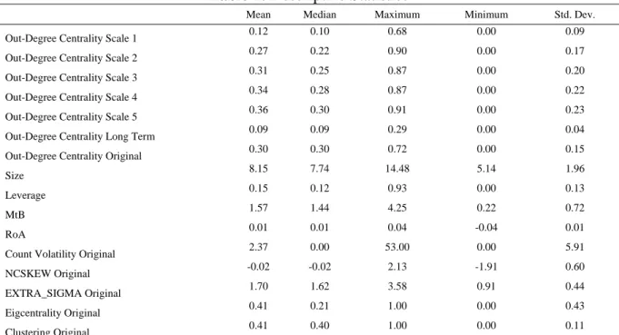
Table 1 presents the descriptive statistics of the out-degree centrality, the Size, the Leverage,

MtB, RoA, COUNT_VOL, NCSKEW, EXTRA_SIGMA, Eigcentrality and Clustering. The

decompositions corresponding to j=1 to 5 regard the corresponding wavelet decompositions, the S index regards the long-term decomposition and the original index regards the actual returns (without decomposition). A closer inspection of Table 1 reveals that the dependent variable is lower for lower scales and increases as the scale increase. This shows that in lower scales the number of nodes affected by the node of interest is lower, likely implying that the low-scale shocks may not persist, while on the contrary, the higher the scale of a shock the higher the probability of persisting in the system.

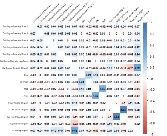
Figure 1 presents a correlation plot of the dependent and independent variables. A closer inspection of Figure 1 reveals correlations very close to zero between the variables with an exception of NCSKEW and EXTRA_SIGMA in the original returns and MtB and RoA.

[Insert Figure 1 approximately here]

5. Empirical Results

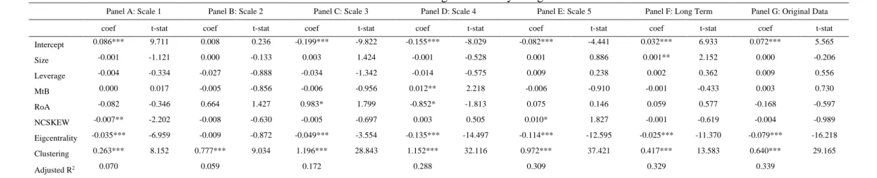
Table 2 presents the results of estimating equation (10), which are used as a benchmark. As it can be seen the coefficient of eigenvector centrality is negative and significant in most cases. This result provides support to Research Hypothesis H2A by showing that the more important

is the neighbor of a node of interest, the more difficult for a shock to pass through him in the network. Moreover, we also see that moving from higher frequencies to lower frequencies (from Panel A to Panel F) the coefficient of eigenvector centrality becomes more negative. This result provides support to Research Hypothesis H2B due to showing that the more

important the nodes connected to the node of interest the less likely that it will affect the change in out-degree centrality as we move to higher scales. Put differently, the higher the measurement scale, the less probable is that a firm will affect its neighbors, if its neighbors are important in the system in the long run.

On the other hand, focusing on the original data (Panel G) we also observe a negative relation between eigenvector centrality and the level of the out-degree centrality, however with a much lower coefficient in relation to other Panels in the Table. The above results confirm the importance of analyzing the contagion in a multiscale framework.

The analysis of the clustering coefficient in Table 2 shows that it is positively related to contagion as measured by the out-degree centrality and thus provides support to Research

(14)

Hypothesis H1A. This result shows that, the more clustered the nodes in the neighbor of a node

of interest, the higher the level of outdegree centrality and hence the more probable is the dissemination of contagion through the system. In addition, we observe higher clustering coefficients to the short- and mid-term components, while we observe a much smaller coefficient in the long-term component. These results provide support to research hypothesis H2B. Again, these results are not reflected at the same extend in the original data, where the

respective coefficient is lower than most of the respective coefficients of the decomposed data. Our results do not indicate any support for H4 since most of the accounting variables are

statistically insignificant for all scales.

[Insert Table 2 approximately here]

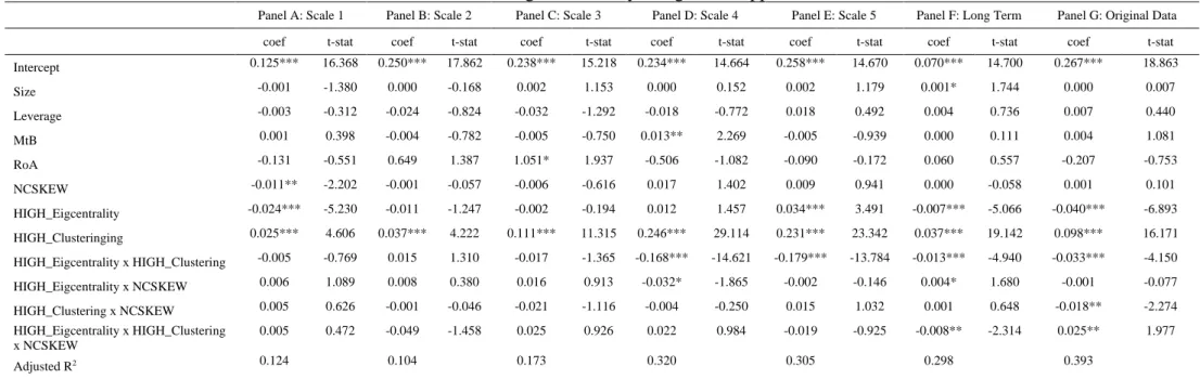
Next, we turn our attention to the results of the extended model reported in Table 3. First, we observe that high eigenvector centrality is related negatively to the out-degree centrality but the respective coefficient is not significant in all Panels of Table 3. High clustering is positively related to out-degree centrality for all scales, as well as, the long-term component and the original data. Its coefficient increases with scale, although it is much smaller for the long-term component and the original data, indicating that a shock originated from a highly clustered banks may affect the system and the magnitude of the effect will be higher in the shock persists in higher scales. These results provide support to Research Hypotheses H1A, H1B, H2A and H2B.

The interaction term between the high centrality and high eigenvector centrality is negative which is expected. Banks that are highly clustered with other banks that are important is more likely to absorb a shock. Also, the coefficient becomes more negative indicating that a shock originating from banks that are highly clustered with high eigenvector centrality in higher scales, is even less probable to spread in the network. Taken together the above results imply that, contagion may be favored by high clustering with important nodes in the network, however, if connectedness is also present in the data then contagion seems to be limited. This implies that neighbors of a node of interest that are important for the system are less prone to contagion if they are also closely connected in triads (have a high clustering coefficient).

(15)

Moreover, firms with a higher likelihood of a stock crash, as measured by the NCSKEW

measure have lower out-degree centrality as shown by the negative and significant coefficient

of NCSKEW but only in Panel A. Moreover, for some of the Panels of Table 3 high eigenvector

centrality leads to a weaker relation between NCSKEW and out-degree centrality. Our results provide some support to Research Hypotheses H3A and H3B but do not provide enough evidence

to support H4 since the coefficients of Size, Leverage, MtB and RoA are statistically

insignificant, with an exception of MtB for scales 3 and 4 and RoA for scale 3.

6. Robustness Checks

In our analysis, the NCSKEW, proposed by Chen et al. (2001), is the prime measure of a shock. For robustness checks, we replace NCSKEW by two alternative crash measures. First, we estimate model (10) using the EXTRA_SIGMA measure of Bradshaw et al. (2010) which is a more extreme measure of crash risk:

 

, , , _ min i w i w i w r r EXTRA SIGMA std r            (13)

For each year, we compute the weekly return that is below the mean weekly return for the specific year, r_{i w}_, , divided by the standard deviation of the weekly returns during the specific year, std r

 

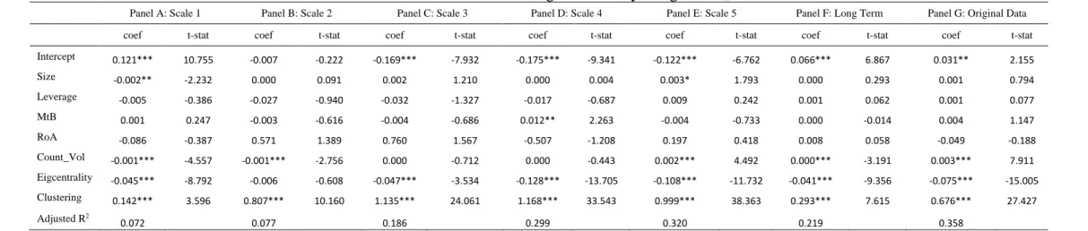
_{i w}_, . The results are presented in the Appendix in Tables A1 and A2 and lead to the same conclusions reached using NCSKEW as the primary measure of crash risk.

Second, we estimate model (10) by replacing the shock measure NSKEW by Count_Vol.

Count_Vol represents the number of times in a year the conditional volatility of a firm is over

the 95th_{quantile of the conditional volatility of all firms. We follow Baur (2012) and estimate}

the conditional volatility using a non-symmetric GARCH model. The results are reported in Tables A3 and A4 in the Appendix and show that our primary conclusions still hold.

7. Conclusions

The present study proposes a novel approach in the measurement of contagion. According to this approach, we use wavelet analysis to decompose stock returns into time scales and then feed these data into a network in order to measure contagion based on the network

(16)

characteristics. In this respect, our approach offers a number of important research insights that would not be unraveled using only the original return series.

Our results show that certain network characteristics like clustering may enhance the contagion effects in some cases, while eigenvector centrality seems to limit it. The effect of both clustering and eigenvector centrality is not constant at different scales but generally increase (in absolute value). The effect of high clustering is more evident in higher scales indicating that a shock originated from a highly clustered banks may affect the system and the magnitude of the effect will be higher in the shock persists in higher scales. On the other hand, when both clustering and eigenvector centrality are high we observe a limiting effect in contagion indicating that a shock originating from banks that are highly clustered with high eigenvector centrality in higher scales it is even less probable to spread in the network. Our results do not provide enough evidence to support the hypothesis that high scale contagion is related positively to more financially healthy firms.

Finally, using wavelet analysis and study contagion in different frequencies we were able to analyze successfully the characteristics of a firm that affect the spread of a shock in the financial markets. This was not possible in the original time-series where the aforementioned effects were masked and our results were often contradicting. These results should be useful to academics and market participants due to the new level of analysis offered by the wavelet decomposition.

References

Acemoglu, D., Ozdaglar, A., and Tahbaz-Salehi, A. (2015). "Systemic Risk and Stability in Financial Networks." American Economic Review 105(2), 564-608.

Alexandridis, A. K., and Zapranis, A. D. (2013). "Wavelet neural networks: A practical guide."

Neural Networks, 42, 1-27.

Alexandridis, A. K., and Zapranis, A. D. (2014). Wavelet Networks: Methodologies and

Applications in Financial Engineering, Classification and Chaos, Wiley, New Jersey,

USA.

Baur, D. G. (2012). "Financial Contagion and the Real Economy." Journal of Banking &

Finance, 36, 2680-2692.

Billio, M., Getmansky, M., Lo, A. W., and Pelizzon, L. (2012). "Econometric Measures of Connectedness and Systemic Risk in the Finance and Insurance Sectors." Journal of

Financial Economics, 104(3), 535-559.

Bradshaw, T., Hutton, A., Marcus, A., and Tehranian, H. (2010). "Opacity, Crash Risk, and the Option Smirk Curve." Available at SSRN: http://ssrn.com/abstract=1640733.

Chen, J., Hong, H., and Stein, J. C. (2001). "Forecasting crashes: trading volume, past returns, and conditional skewness in stock prices." Journal of Financial Economics, 61(3), 345-381.

(17)

Conlon, T., and Cotter, J. (2012). "An empirical analysis of dynamic multiscale hedging using wavelet decomposition." Journal of Futures Markets, 32(3), 272-299.

Conlon, T., Cotter, J., and Gençay, R. (2016). "Commodity futures hedging, risk aversion and the hedging horizon." The European Journal of Finance, 22(15), 1534-1560.

Dimson, E. (1979). "Risk measurement when shares are subject to infrequent trading." Journal

of Financial Economics, 7(2), 197-226.

Donoho, D. L., and Johnstone, I. M. (1994). "Ideal Spatial Adaption by Wavelet Shrinkage."

Biometrika, 81, 425-455.

Elliott, M., Golub, B., and Jackson, M. O. (2014). " Financial Networks and Contagion." Available at SSRN: http://ssrn.com/abstract=2175056 or

http://dx.doi.org/10.2139/ssrn.2175056.

Fagiolo, G. (2007). "Clustering in complex directed networks." Physical Review E, 76(2), 026107.

Fernandez, V. (2006). "The CAPM and value at risk at different time-scales." International

Review of Financial Analysis, 15(3), 203-219.

Gençay, R., Selçuk, F., and Whitcher, B. (2005). "Multiscale systematic risk." Journal of

International Money and Finance, 24(1), 55-70.

Granger, C. W. J. (1969). "Investigating Causal Relations by Econometric Models and Cross-Spectral Methods." Econometrica: Journal of the Econometric Society, 424-438. In, F., and Kim, S. (2006). "The hedge ratio and the empirical relationship between the stock

and futures markets: A new approach using wavelet analysis." Journal of Business, 79(2), 799-820.

Kim, S., and In, F. (2005). "The Relationship between Stock Returns and Inflation: New Evidence from Wavelet Analysis." Journal of Empirical Finance, 12(3), 435-444. Mallat, S. G. (1999). A Wavelet Tour of Signal Processing, Academic Press, San Diego. Mantegna, R. N. (1999). "Hierarchical Structure in Financial Markets." The European Physical

Journal B-Condensed Matter and Complex Systems, 11(1), 193-197.

Newman, M. (2010). Networks: an introduction, Oxford university press.

Onnela, J. P., Kaski, K., and Kertész, J. (2004). "Clustering and Information in Correlation based Financial Networks." The European Physical Journal B-Condensed Matter and

Complex Systems, 38(2), 353-362.

Percival, D., and Walden, A. (2000). Wavelets analysis for time series analysis, Cambridge University Press, Cambridge, U.K.

Ramsey, J. B. (1999). "The contribution of wavelets to the analysis of economic and financial data." Philosophical Transactions of the Royal Society of London A: Mathematical,

Physical and Engineering Sciences, 357(1760), 2593-2606.

Reboredo, J. C., and Rivera-Castro, M. A. (2014). "Wavelet-Based Evidence of the Impact of Oil Prices on Stock Returns." International Review of Economics & Finance, 29, 145-176.

Tumminello, M., Aste, T., Di Matteo, T., and Mantegna, R. N. (2005). "A Tool for Filtering Information in Complex Systems." Proceedings of the National Academy of Sciences

of the United States of America, 102(30), 10421-10426.

Watts, D. J., and Strogatz, S. H. (1998). "Collective dynamics of'small-world'networks."

(18)

Table 1: Descriptive Statistics

Mean Median Maximum Minimum Std. Dev.

Out-Degree Centrality Scale 1 0.12 0.10 0.68 0.00 0.09

Out-Degree Centrality Long Term 0.09 0.09 0.29 0.00 0.04

Out-Degree Centrality Original 0.30 0.30 0.72 0.00 0.15

Size 8.15 7.74 14.48 5.14 1.96

Leverage 0.15 0.12 0.93 0.00 0.13

MtB 1.57 1.44 4.25 0.22 0.72

RoA 0.01 0.01 0.04 -0.04 0.01

Count Volatility Original 2.37 0.00 53.00 0.00 5.91

NCSKEW Original -0.02 -0.02 2.13 -1.91 0.60

EXTRA_SIGMA Original 1.70 1.62 3.58 0.91 0.44

Eigcentrality Original 0.41 0.21 1.00 0.00 0.43

Clustering Original 0.41 0.40 1.00 0.00 0.11

Notes: The sample covers the period 1997-2016 and concern 240 US banks with 4,140 observations. Scales 1 to 5 concern the decomposition of idiosyncratic returns using the wavelet analysis and the associated Out-Degree Centrality, using the j=1 to 5 return decompositions, which serve as the proxy of contagion.

(19)

Table 2: Determinants of out-degree centrality using NCSKEW

Panel A: Scale 1 Panel B: Scale 2 Panel C: Scale 3 Panel D: Scale 4 Panel E: Scale 5 Panel F: Long Term Panel G: Original Data

coef t-stat coef t-stat coef t-stat coef t-stat coef t-stat coef t-stat coef t-stat

Intercept 0.086*** 9.711 0.008 0.236 -0.199*** -9.822 -0.155*** -8.029 -0.082*** -4.441 0.032*** 6.933 0.072*** 5.565 Size -0.001 -1.121 0.000 -0.133 0.003 1.424 -0.001 -0.528 0.001 0.886 0.001** 2.152 0.000 -0.206 Leverage -0.004 -0.334 -0.027 -0.888 -0.034 -1.342 -0.014 -0.575 0.009 0.238 0.002 0.362 0.009 0.556 MtB 0.000 0.017 -0.005 -0.856 -0.006 -0.956 0.012** 2.218 -0.006 -0.910 -0.001 -0.433 0.003 0.730 RoA -0.082 -0.346 0.664 1.427 0.983* 1.799 -0.852* -1.813 0.075 0.146 0.059 0.577 -0.168 -0.597 NCSKEW -0.007** -2.202 -0.008 -0.630 -0.005 -0.697 0.003 0.505 0.010* 1.827 -0.001 -0.619 -0.004 -0.989 Eigcentrality -0.035*** -6.959 -0.009 -0.872 -0.049*** -3.554 -0.135*** -14.497 -0.114*** -12.595 -0.025*** -11.370 -0.079*** -16.218 Clustering 0.263*** 8.152 0.777*** 9.034 1.196*** 28.843 1.152*** 32.116 0.972*** 37.421 0.417*** 13.583 0.640*** 29.165 Adjusted R2 0.070 0.059 0.172 0.288 0.309 0.329 0.339

(20)

Table 3: Determinants of out-degree centrality using a DiD approach and NCSKEW

Intercept 0.125*** 16.368 0.250*** 17.862 0.238*** 15.218 0.234*** 14.664 0.258*** 14.670 0.070*** 14.700 0.267*** 18.863 Size -0.001 -1.380 0.000 -0.168 0.002 1.153 0.000 0.152 0.002 1.179 0.001* 1.744 0.000 0.007 Leverage -0.003 -0.312 -0.024 -0.824 -0.032 -1.292 -0.018 -0.772 0.018 0.492 0.004 0.736 0.007 0.440 MtB 0.001 0.398 -0.004 -0.782 -0.005 -0.750 0.013** 2.269 -0.005 -0.939 0.000 0.111 0.004 1.081 RoA -0.131 -0.551 0.649 1.387 1.051* 1.937 -0.506 -1.082 -0.090 -0.172 0.060 0.557 -0.207 -0.753 NCSKEW -0.011** -2.202 -0.001 -0.057 -0.006 -0.616 0.017 1.402 0.009 0.941 0.000 -0.058 0.001 0.101 HIGH_Eigcentrality -0.024*** -5.230 -0.011 -1.247 -0.002 -0.194 0.012 1.457 0.034*** 3.491 -0.007*** -5.066 -0.040*** -6.893 HIGH_Clusteringing 0.025*** 4.606 0.037*** 4.222 0.111*** 11.315 0.246*** 29.114 0.231*** 23.342 0.037*** 19.142 0.098*** 16.171 HIGH_Eigcentrality x HIGH_Clustering -0.005 -0.769 0.015 1.310 -0.017 -1.365 -0.168*** -14.621 -0.179*** -13.784 -0.013*** -4.940 -0.033*** -4.150 HIGH_Eigcentrality x NCSKEW 0.006 1.089 0.008 0.380 0.016 0.913 -0.032* -1.865 -0.002 -0.146 0.004* 1.680 -0.001 -0.077 HIGH_Clustering x NCSKEW 0.005 0.626 -0.001 -0.046 -0.021 -1.116 -0.004 -0.250 0.015 1.032 0.001 0.648 -0.018** -2.274 HIGH_Eigcentrality x HIGH_Clustering x NCSKEW 0.005 0.472 -0.049 -1.458 0.025 0.926 0.022 0.984 -0.019 -0.925 -0.008** -2.314 0.025** 1.977 Adjusted R2 0.124 0.104 0.173 0.320 0.305 0.298 0.393

(21)

(22)

Appendix

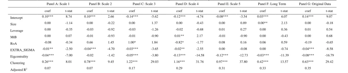
Table A1: Determinants of out-degree centrality using EXTRA_SIGMA

Intercept 0.10*** 8.74 0.10*** 2.66 -0.14*** -5.62 -0.12*** -4.74 -0.08*** -3.54 0.03*** 6.07 0.14*** 9.07 Size 0.00 -1.14 0.00 -0.22 0.00 1.37 0.00 -0.43 0.00 0.89 0.00** 2.13 0.00 -0.18 Leverage 0.00 -0.35 -0.03 -0.92 -0.03 -1.26 -0.02 -0.68 0.01 0.27 0.00 0.36 0.01 0.54 MtB 0.00 0.07 -0.01 -0.93 -0.01 -0.90 0.01** 2.17 -0.01 -0.90 0.00 -0.43 0.00 0.68 RoA -0.08 -0.34 0.66 1.45 1.00* 1.84 -0.82* -1.77 0.08 0.16 0.06 0.59 -0.19 -0.65 EXTRA_SIGMA -0.01** -2.50 -0.04*** -4.70 -0.03*** -3.65 -0.02** -2.55 0.00 -0.08 0.00 -0.74 -0.04*** -8.58 Eigcentrality -0.04*** -7.00 -0.02 -1.42 -0.05*** -3.80 -0.13*** -14.58 -0.12*** -12.73 -0.03*** -11.39 -0.08*** -16.79 Clustering 0.26*** 8.01 0.78*** 9.45 1.22*** 29.03 1.16*** 31.76 0.97*** 37.80 0.42*** 13.57 0.63*** 29.42 Adjusted R2 0.07 0.07 0.17 0.29 0.31 0.33 0.35

(23)

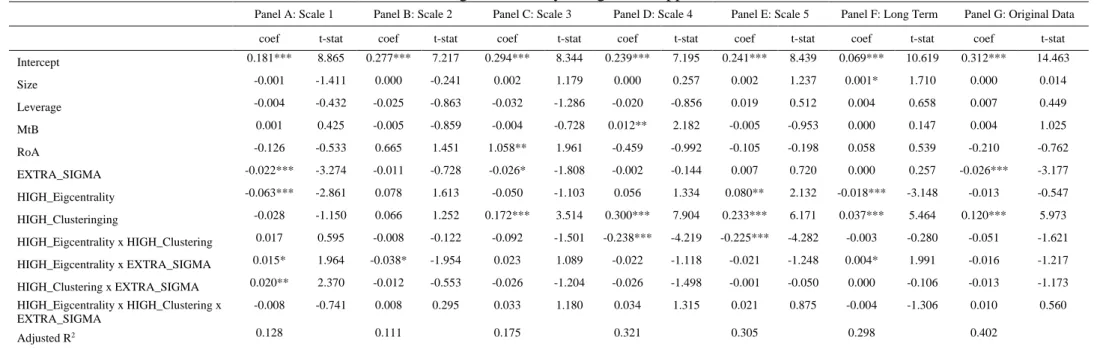
Table A2: Determinants of out-degree centrality using a DiD approach and EXTRA_SIGMA

Intercept 0.181*** 8.865 0.277*** 7.217 0.294*** 8.344 0.239*** 7.195 0.241*** 8.439 0.069*** 10.619 0.312*** 14.463 Size -0.001 -1.411 0.000 -0.241 0.002 1.179 0.000 0.257 0.002 1.237 0.001* 1.710 0.000 0.014 Leverage -0.004 -0.432 -0.025 -0.863 -0.032 -1.286 -0.020 -0.856 0.019 0.512 0.004 0.658 0.007 0.449 MtB 0.001 0.425 -0.005 -0.859 -0.004 -0.728 0.012** 2.182 -0.005 -0.953 0.000 0.147 0.004 1.025 RoA -0.126 -0.533 0.665 1.451 1.058** 1.961 -0.459 -0.992 -0.105 -0.198 0.058 0.539 -0.210 -0.762 EXTRA_SIGMA -0.022*** -3.274 -0.011 -0.728 -0.026* -1.808 -0.002 -0.144 0.007 0.720 0.000 0.257 -0.026*** -3.177 HIGH_Eigcentrality -0.063*** -2.861 0.078 1.613 -0.050 -1.103 0.056 1.334 0.080** 2.132 -0.018*** -3.148 -0.013 -0.547 HIGH_Clusteringing -0.028 -1.150 0.066 1.252 0.172*** 3.514 0.300*** 7.904 0.233*** 6.171 0.037*** 5.464 0.120*** 5.973 HIGH_Eigcentrality x HIGH_Clustering 0.017 0.595 -0.008 -0.122 -0.092 -1.501 -0.238*** -4.219 -0.225*** -4.282 -0.003 -0.280 -0.051 -1.621 HIGH_Eigcentrality x EXTRA_SIGMA 0.015* 1.964 -0.038* -1.954 0.023 1.089 -0.022 -1.118 -0.021 -1.248 0.004* 1.991 -0.016 -1.217 HIGH_Clustering x EXTRA_SIGMA 0.020** 2.370 -0.012 -0.553 -0.026 -1.204 -0.026 -1.498 -0.001 -0.050 0.000 -0.106 -0.013 -1.173 HIGH_Eigcentrality x HIGH_Clustering x EXTRA_SIGMA -0.008 -0.741 0.008 0.295 0.033 1.180 0.034 1.315 0.021 0.875 -0.004 -1.306 0.010 0.560 Adjusted R2 0.128 0.111 0.175 0.321 0.305 0.298 0.402

(24)

Table A3: Determinants of out-degree centrality using Count_Vol

Intercept _0.121*** _10.755 _-0.007 _-0.222 _-0.169*** _-7.932 _-0.175*** _-9.341 _-0.122*** _-6.762 _0.066*** _6.867 _0.031** _2.155 Size _-0.002** _-2.232 _0.000 _0.091 _0.002 _1.210 _0.000 _0.004 _0.003* _1.793 _0.000 _0.293 _0.001 _0.794 Leverage _-0.005 _-0.386 _-0.027 _-0.940 _-0.032 _-1.327 _-0.017 _-0.687 _0.009 _0.242 _0.001 _0.062 _0.001 _0.077 MtB _0.001 _0.247 _-0.003 _-0.616 _-0.004 _-0.686 _0.012** _2.263 _-0.004 _-0.733 _0.000 _-0.014 _0.004 _1.147 RoA _-0.086 _-0.387 _0.571 _1.389 _0.760 _1.567 _-0.507 _-1.208 _0.197 _0.418 _0.008 _0.058 _-0.049 _-0.188 Count_Vol _-0.001*** _-4.557 _-0.001*** _-2.756 _0.000 _-0.712 _0.000 _-0.443 _0.002*** _4.492 _0.000*** _-3.191 _0.003*** _7.911 Eigcentrality _-0.045*** _-8.792 _-0.006 _-0.608 _-0.047*** _-3.534 _-0.128*** _-13.705 _-0.108*** _-11.732 _-0.041*** _-9.356 _-0.075*** _-15.005 Clustering _0.142*** _3.596 _0.807*** _10.160 _1.135*** _24.061 _1.168*** _33.543 _0.999*** _38.363 _0.293*** _7.615 _0.676*** _27.427 Adjusted R2 0.072 0.077 0.186 0.299 0.320 0.219 0.358

(25)

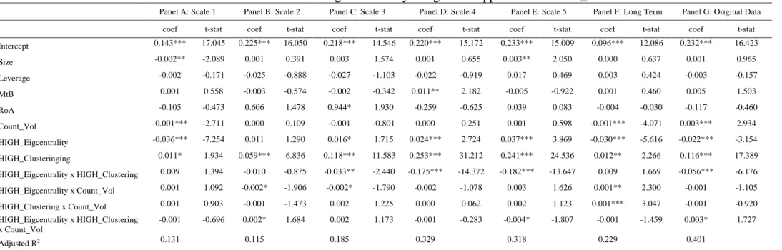
Table A4: Determinants of out-degree centrality using a DiD approach and Count_Vol

Intercept 0.143*** 17.045 0.225*** 16.050 0.218*** 14.546 0.220*** 15.172 0.233*** 15.009 0.096*** 12.086 0.232*** 16.423 Size -0.002** -2.089 0.001 0.391 0.003 1.574 0.001 0.655 0.003** 2.050 0.000 0.637 0.001 0.965 Leverage -0.002 -0.171 -0.025 -0.888 -0.027 -1.103 -0.022 -0.919 0.017 0.469 0.003 0.424 -0.003 -0.157 MtB 0.001 0.558 -0.003 -0.574 -0.002 -0.342 0.011** 2.182 -0.005 -0.922 0.001 0.460 0.005 1.503 RoA -0.105 -0.473 0.606 1.478 0.944* 1.930 -0.259 -0.625 0.039 0.083 -0.004 -0.030 -0.117 -0.460 Count_Vol -0.001*** -2.711 0.000 0.109 -0.001 -0.801 0.000 0.251 0.001 0.598 -0.001*** -4.071 0.003*** 2.934 HIGH_Eigcentrality -0.036*** -7.254 0.011 1.290 0.016* 1.715 0.024*** 2.724 0.037*** 3.869 -0.030*** -5.616 -0.022*** -3.154 HIGH_Clusteringing 0.011* 1.934 0.059*** 6.836 0.118*** 11.583 0.253*** 31.212 0.241*** 24.536 0.012** 2.266 0.116*** 17.389 HIGH_Eigcentrality x HIGH_Clustering 0.009 1.394 -0.010 -0.875 -0.033** -2.440 -0.175*** -14.372 -0.182*** -13.647 0.009 1.669 -0.056*** -6.176 HIGH_Eigcentrality x Count_Vol 0.001 1.092 -0.002* -1.906 -0.002* -1.790 -0.002 -1.078 0.003 1.626 0.001** 2.300 -0.001 -1.105 HIGH_Clustering x Count_Vol 0.001 0.903 -0.001 -1.473 0.002 1.225 0.000 0.062 0.002 1.123 0.001*** 3.047 -0.001 -0.920 HIGH_Eigcentrality x HIGH_Clustering x Count_Vol -0.001 -0.696 0.002* 1.684 0.002 1.173 -0.001 -0.283 -0.004* -1.807 -0.001 -1.459 0.003* 1.727 Adjusted R2 0.131 0.115 0.185 0.329 0.318 0.229 0.401

:

http://ssrn.com/abstract=2175056

http://dx.doi.org/10.2139/ssrn.2175056.