COVID-19 second wave mortality in Europe and the United States
Nick James,1Max Menzies,2,a)and Peter Radchenko3
1)School of Mathematics and Statistics, University of Sydney, NSW, 2006, Australia 2)Yau Mathematical Sciences Center, Tsinghua University, Beijing, 100084, China 3)School of Business, University of Sydney, NSW, 2006, Australia
(Dated: 4 August 2020)
This paper introduces new methods to analyze the changing progression of COVID-19 cases to deaths in different waves of the pandemic. First, an algorithmic approach partitions each country or state’s COVID-19 time series into a first wave and subsequent period. Next, offsets between case and death time series are learned for each country via a normalized inner product. Combining these with additional calculations, we can determine which countries have most substantially reduced the mortality rate of COVID-19. Finally, our paper identifies similarities in the trajectories of cases and deaths for European countries and U.S. states. Our analysis refines the popular conception that the mortality rate has greatly decreased throughout Europe during its second wave of COVID-19; instead, we demonstrate a bifurcation in which wealthier Western European countries have managed their mortality rate more successfully. A similar distinction exists in the United States, where Northeastern states have been the most successful in the country.
Europe is experiencing a substantial second wave of COVID-19. Epidemiologists have attributed this to loos-ening of both government restrictions and individual precautions.1This reflects the ongoing struggle to balance the spread of the virus and allowing public life to return to normal, a year into the pandemic.2The mortality rate of the disease, and how it changes over time, plays a critical role in this debate. Identifying countries that have reduced their mortality rate in subsequent waves of the disease is therefore of great relevance to policymakers. In the pub-lic conception, health experts and journalists alike have noted a substantial decrease in the mortality of COVID-19 in Europe’s second wave.3This paper aims to refine this conception with a mathematical analysis on a country-by-country basis. Instead, we show a considerable variance in the reduction of mortality in different countries’ second waves. Most wealthy countries in Europe, with the notable exceptions of Germany and Sweden, have drastically re-duced their mortality rate during their second wave. Less wealthy European countries, as well as many U.S. states, have seen a less notable reduction.
I. INTRODUCTION
Government responses to COVID-19 have varied substan-tially, both from country to country and as time has progressed. Early responses included banning travel4and establishing test and trace programs,5followed by lockdowns as cases rose, of-ten implemented too late.6,7Due to the economic consequences and unpopularity of lockdowns, the U.S. states prioritized re-opening well before the virus was entirely suppressed.8Such responses to the virus, highly varying with time, have created
first and subsequent wavesof the outbreak in most countries, with subsequent waves often exhibiting greater case numbers than the first.9,10
a)Electronic mail: [email protected]
Fortunately, subsequent waves of COVID-19 have featured a reduced mortality rate in many countries.11Explanations for this include the development of new treatments for COVID-19 as time passes12–15and under-reporting of true case numbers in the first wave.16This paper is the first to perform a math-ematical analysis to quantify the reduction of mortality on a country-by-country basis throughout Europe, and compare Eu-ropean countries with U.S. states. We demonstrate significant heterogeneity in Europe, with wealthier Western European countries having reduced their mortality rate more drastically than less wealthy European countries or U.S. states.
To perform our analysis, we use new and recently intro-duced techniques intime series analysis. Time series analysis has been frequently used in epidemiology,17,18 including to study the Zika virus,19,20Ebola,21,22and COVID-19.23–26 Non-linear dynamics researchers apply a wide range of methods, including power-law models,23,26,27distance analysis,10,28–31 and network models.32,33In this work, we apply the algorith-mic framework introduced in Ref. 10 to partition COVID-19 case time series into a first wave and a subsequent period (the latter could consist of a single second wave or multiple waves). Later, we consider all the European countries and U.S. states in conjunction, and identify similarities in their case and death trajectories viaclustering. We implementhierarchical clustering; this technique has been used in a wide variety of epidemiological applications.24,34–38
This paper is structured as follows: in Section II, we study the reduction in mortality rate between the first and subsequent waves of COVID-19 among European countries and U.S. states. This relies on a new framework for partitioning time series and learning appropriate offsets. In Section III, we study all European countries and U.S. states in conjunction, clustering case and death trajectories to elucidate similarities across the two groups. We summarize our findings regarding COVID-19 mortality and trajectories across first and subsequent waves in Section IV.
In this section, we describe a mathematical framework to analyze the changing mortality relative to first and subsequent waves of COVID-19. We first apply our constructions on an individual country-by-country basis and then collectively compare all the European countries and U.S. states. Our list of European countries comes from the United Nations,39except we exclude Russia and the Holy See. We consider all U.S. states plus the District of Columbia (D.C.). This gives us 93 total countries and states.
A. Methodology: determination of offsets and mortality
ratios
Letx(t),y(t)be the new daily case and death time series, respectively, of a single country or state,t=0, ...,T. In this paper, data for every country and state spans 01/21/2020 to 11/25/2020, a period of 310 days. The end date corresponds to the last week that the European Centre for Disease Prevention and Control (ECDC) provided daily data updates.40That is,
T =309 for every time series.
First, we apply the methodology developed in Ref. 10 to divide each country into first and subsequent waves of the disease. Specifically, we apply a smoothing filter to the case time seriesx(t)followed by a two-step algorithm to output an alternating sequence of local maxima (peaks) and minima (troughs), beginning with a trough att=0, where there are zero cases. Further details are provided in Appendix A. We apply this only to the case counts, as the death counts are much sparser. Just two European countries and three U.S. states in our analysis are assigned a sequence that consists of just one trough att=0, and one peak. These countries and states are determined to still be in their first wave of COVID-19. For every other country, we have at least one non-trivial trough. LetT1be the first non-trivial trough, or the second trough after
t=0. This marks the end of the complete first wave in the corresponding country. We refer to the periodt=0, ...,T1as the first wave, andt=T1+1, ...,T as the subsequent period.
We aim to analyze the changing mortality rate by comparing the first wave and the subsequent period. Indeed, we wish to understand if countries were able to learn and adapt their treatment of the disease after the end of the first wave. To appropriately compare the case and death time series, we must calculate an offset in time between cases and deaths for each country. For this purpose, we usenormalized inner products, and can either assume that there is a single offset for the entire time period, or two offsets - one each for the first wave and subsequent period.
For each country, letτbe the optimal single offset between the case and death time series. We define this as the optimal value of the normalized inner product
<x(0 :T−τ),y(τ:T)>n= (1)
x(0)y(τ) +...+x(T−τ)y(T)
(x(0)2+...+x(T−τ)2)21(y(τ)2+...+y(T)2)12
. (2)
imal value 1 if and only if there is a proportionality relation
y(t) =kx(t+τ)for allt=0, ...,T−τfor some constantk>0. Indeed, we are seeking the offset in time where deaths are most closely proportional to cases. This is more suitable than other metrics, such as correlation or distance correlation.29 Correla-tion or distance correlaCorrela-tion would each return maximal value 1 ify=kx+bfor an additional constantb, which is unsuitable.
Having determined this offset, we can define
M1=∑ T1+τ t=τ y(t) ∑Tt=10x(t) , (3) M2= ∑tT=T1+1+τy(t) ∑tT=−Tτ1+1x(t) . (4)
These record the mortality rates for each country over the first wave and subsequent period, respectively, taking into account a single offset between case and death counts.
Alternatively, we can determine a pair of two offsetsλ1and λ2. The first offsetλ1is chosen to maximize the normalized inner product
<x(0 :T1),y(λ1:T1+λ1)>n. (5) while the second offsetλ2is chosen to maximize the normal-ized inner product
<x(T1+1 :T−λ2),y(T1+λ2:T)>n. (6) With these two offsets, we can define
N1= ∑tT=1+λλ1 1 y(t) ∑Tt=10x(t) , (7) N2= ∑tT=T1+1+λ2y(t) ∑tT=−Tλ12+1x(t) . (8)
These record the mortality rates for each country over the first wave and subsequent period, respectively, taking into account two respective offsets between case and death counts. Each country or state is assigned its own value of
T1,τ,M1,M2,λ1,λ2,N1,N2, whileT =309 is fixed for all of them. We refer toτ,λ1,λ2asoffsetsandM1/M2andN1/N2as
one- and two-offset mortality ratios, respectively.
Finally, we can generate convenient scatter plots to show the case and death counts of the first wave and the subsequent period. Using the two offsetsλ1,λ2, we can simply plot the set of first wave values{(x(t),y(t+λ1))∈R2:t=0, ...,T1} and subsequent period values {(x(t),y(t+λ2))∈R2:t = T1, ...,T−λ2}. In the next section, we plot these two peri-ods in red and blue, respectively, and include their centroid (that is, average) and convex hull.41
(a) (b) (c)
(d) (e) (f)
FIG. 1: Smoothed case time series and identified turning points for various European countries: (a) the United Kingdom (b) France (c) Germany (d) Sweden (e) Romania (f) Belarus. Green and red vertical lines denote algorithmically detected troughs and
peaks, respectively.
(a) (b) (c)
(d) (e) (f)
FIG. 2: Scatter plots of cases and deaths for the first wave and subsequent period, for (a) the United Kingdom (b) France (c) Germany (d) Sweden (e) Romania (f) Belarus. The first wave data is plotted in red, the subsequent period in blue, with two offsets
Figure 1 displays new case time series and algorithmically determined turning points (peaks and troughs) for six European countries. The first non-trivial troughT1splits each time series up into its first wave and subsequent period. All these countries display a similar structure - they experience a first wave in cases followed by at least one more significant subsequent wave. The United Kingdom (U.K.), France and Germany, displayed in Figures 1a, 1b, and 1c, respectively, highlight a characteristic case trajectory for wealthier European countries, in which there are two predominant waves in COVID-19 cases. Less developed European countries such as Romania and Belarus, displayed in Figures 1e and 1f, respectively, produce a similar new case trajectory to the wealthier European countries, yet many with a smaller first wave, like Romania.
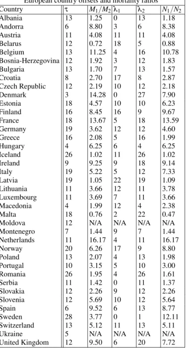
In Tables I and II, respectively, we record the values ofτ,
M1/M2, λ1,λ2and N1/N2 for European countries and U.S. states, respectively. First, we notice significant variance be-tween European countries in the one-offset mortality ratios
M1/M2. The Netherlands has the highest ratio of 16.2, fol-lowed by Denmark, France, Belgium, Spain, the U.K., Ireland, Andorra, Finland and Norway, all of which are wealthy coun-tries in Western or Northern Europe. These councoun-tries are indi-cated to have drastically reduced COVID-19 mortality between their first wave and subsequent period. By contrast, the small-est mortality ratios are exhibited by Belarus, Malta, Iceland, Latvia, Albania and Serbia, most of which are less developed. Notable wealthy countries with comparatively low mortality ratios include Germany (3.6) and Sweden (3.8). These coun-tries have not reduced their mortality ratio as much relative to their first wave.
We obtain broadly similar results in the two-offset mortality ratiosN1/N2. Once again, the Netherlands has the highest ratio, followed by France, Sweden, Belgium, Finland, Ireland, Norway, Spain, Andorra, Denmark and the U.K. Sweden has changed its position drastically due to significant differences in the optimized values ofτ,λ1,λ2. Malta, Belarus, Iceland, Latvia, Albania and Serbia have the lowest two-offset mortality ratios. Broadly, but not universally, the two methods give similar results, indicating the robustness of the methodology.
Such heterogeneity is also observed for the United States. The U.S. states with the greatest one-offset mortality ratio are Vermont (9.2), New Jersey, New York and Connecticut, all Northeastern states, with similar results observed for the two-offset mortality ratio. No U.S. state reduced its mortality as much as the Netherlands, Denmark, France, Belgium, Spain, the U.K. or Ireland.
We can further elucidate the differences between first and subsequent wave mortality by examining the case-death scatter plots in Figure 2. As described in Section II A, we plot both first and subsequent waves accounting for two offsets, and include the centroid and convex hull of each set, understood as a subset ofR2. The U.K., France, Germany and Sweden, displayed in Figures 2a, 2b, 2c and 2d, respectively, show a similar pattern. These countries experience a significantly higher mortality rate during their first wave than subsequent period. This finding is consistent among many of the more
de-of the scatter plot regions is sharper for the U.K. and France than for Germany and Sweden, consistent with their mortality ratios. The pattern among several less developed European countries such as Romania and Belarus is markedly different, as seen in Figures 2e and 2f. Romania is one of several eastern European countries with a smaller first wave, while Belarus exhibits no real change in the progression from cases to deaths at all.
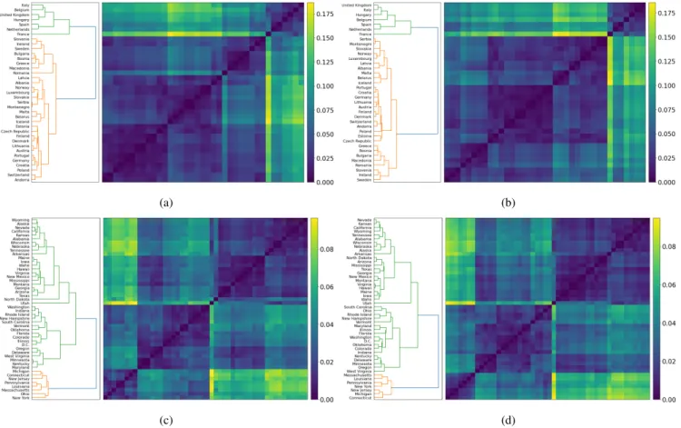
We extend our analysis of mortality by implementing hier-archical clustering on the ordered pairs(M1,M2)and(N1,N2), understood as elements ofR2. We retain more information this
way without taking the quotients. Figures 3a and 3b demon-strate a consistent structure among European countries across both our one offset and two offset models. Both figures con-tain two clusters; a smaller cluster and a larger cluster with two sub-clusters. In each dendrogram, the smaller cluster con-tains the same members, Belgium, France, Hungary, Italy, the Netherlands, Spain and the U.K. Excluding Hungary, these countries have much in common. They are all wealthy west-ern European countries that have among the highestM1/M2 andN1/N2ratios. They experienced severe first waves in both cases and deaths and implemented harsh lockdown procedures in response. Even Hungary has comparatively high mortality ratios relative to the rest of Europe.
Figures 3c and 3d display the cluster structure among U.S. states, with striking similarities to the European countries. Once again, there are two clusters in each figure, one larger cluster with two subclusters and one smaller cluster. Again, the smaller cluster highlights a collection of anomalous states, predominantly located in the Northeastern United States. Con-necticut, Massachusetts, New Jersey, New York, and Pennsyl-vania feature in both smaller clusters. Like western Europe, these states experienced early and severe first waves. There is a consistent theme among European countries and U.S. states -countries and states that were impacted most severely during the first wave have managed the progression from cases to deaths more successfully in subsequent waves.
To understand this phenomenon further, we divided the Eu-ropean countries into two similarly sized groups based on the total number of cases in the first wave, adjusted for the population. As with Table I, we exclude the three smallest European countries Liechtenstein, Monaco and San Marino, in addition to Moldova and Ukraine, which are determined to still be in their first wave. The group that experienced a more substantial first wave (more than 1.5 total first wave cases per 1000 of population) consisted of 18 countries: Andorra, Austria, Belarus, Belgium, Denmark, France, Germany, Italy, Iceland, Ireland, Luxembourg, the Netherlands, Norway, Por-tugal, Spain, Sweden, Switzerland, and the U.K. The second group, which experienced a smaller first wave (less than 1.5 cases per 1000 population) was comprised of the following 19 countries: Albania, Bosnia and Herzegovina, Bulgaria, Croatia, Czech Republic, Estonia, Finland, Greece, Hungary Latvia, Lithuania, Macedonia, Malta, Montenegro, Poland, Serbia, Slovenia, and Slovakia. The averageN1/N2ratio for the first group was 7.39, while the same ratio for the second group was 2.94, illustrating that the first group had a more substantial
European country offsets and mortality ratios Country τ M1/M2λ1 λ2 N1/N2 Albania 13 1.25 0 13 1.18 Andorra 6 8.80 3 6 8.38 Austria 11 4.08 11 11 4.08 Belarus 12 0.72 18 5 0.88 Belgium 13 11.25 4 16 10.78 Bosnia-Herzegovina 12 1.92 3 12 1.83 Bulgaria 13 1.70 7 13 1.57 Croatia 8 2.70 17 8 2.87 Czech Republic 12 2.19 10 12 2.18 Denmark 3 14.28 0 27 7.90 Estonia 18 4.57 10 10 6.23 Finland 16 8.45 16 9 9.67 France 18 13.67 5 18 13.59 Germany 19 3.62 12 12 4.60 Greece 16 2.08 5 16 1.99 Hungary 4 6.25 6 4 6.25 Iceland 26 1.02 11 26 1.02 Ireland 9 9.25 9 18 9.14 Italy 19 5.22 5 12 7.33 Latvia 19 1.05 22 19 1.09 Lithuania 11 3.66 12 11 3.78 Luxembourg 11 3.69 7 11 3.66 Macedonia 4 1.99 12 4 2.38 Malta 18 0.76 2 22 0.47
Moldova 12 N/A N/A N/A N/A
Montenegro 7 1.44 9 7 1.44 Netherlands 11 16.17 4 11 16.17 Norway 20 6.26 17 9 8.80 Poland 13 2.07 4 13 1.98 Portugal 10 3.15 5 10 3.00 Romania 26 1.95 4 26 1.61 Serbia 11 1.42 0 11 1.37 Slovakia 12 2.26 9 12 2.26 Slovenia 12 5.69 10 12 5.64 Spain 6 9.52 6 13 8.77 Sweden 28 3.77 0 1 12.11 Switzerland 13 5.12 11 13 5.11
Ukraine 5 N/A N/A N/A N/A
United Kingdom 12 9.50 6 20 7.72
TABLE I: European countries and their estimated offsets and mortality ratios, as defined in Section II A. Moldova and Ukraine are determined to be in their first wave, and so do not
have values ofT1,Mi,Niorλi. The three smallest countries Liechtenstein, Monaco and San Marino are excluded.
decrease in the mortality rate between the first wave and subse-quent period. We confirmed the statistical significance of the aforementioned difference in theN1/N2ratio via a two-sample t-test, which had ap-value of 0.0005. We conducted a similar analysis for the U.S. states however we did not reach the same conclusions. In fact, the second group of U.S. states (which experienced a smaller first wave of cases) had a slightly greater decrease in the mortality rate than the first group of states (the difference was not statistically significant). We observed the
U.S. state offsets and mortality ratios
State τ M1/M2λ1 λ2 N1/N2 Alabama 18 1.13 4 18 1.06 Alaska 29 3.36 3 16 4.07 Arizona 13 1.39 13 20 1.26 Arkansas 11 0.69 25 26 0.72 California 13 1.62 6 27 1.36 Colorado 25 3.81 5 5 7.01 Connecticut 13 6.67 6 13 6.62 Delaware 6 2.52 9 21 2.66 D.C. 6 4.27 6 19 4.10 Florida 19 2.84 11 19 2.61 Georgia 29 1.30 13 3 1.30 Hawaii 27 1.90 8 27 1.90 Idaho 13 3.21 11 13 3.12 Illinois 19 3.42 5 12 4.00 Indiana 18 3.76 4 11 4.29 Iowa 18 2.52 7 18 2.40 Kansas 6 2.24 3 6 2.20 Kentucky 13 3.91 5 27 3.06 Louisiana 13 3.63 11 20 3.56 Maine 6 2.79 9 10 2.51 Maryland 11 3.81 4 4 4.08 Massachusetts 12 2.49 4 6 2.80 Michigan 20 4.78 6 13 5.85 Minnesota 12 4.15 4 12 3.99 Mississippi 13 1.62 6 13 1.56
Missouri 40 N/A N/A N/A N/A
Montana 14 2.40 3 14 2.10 Nebraska 13 1.63 5 13 1.55 Nevada 18 1.65 18 13 1.82 New Hampshire 26 3.13 12 26 3.09 New Jersey 11 8.23 11 13 7.51 New Mexico 13 1.88 5 13 1.81 New York 5 7.41 2 17 5.97
North Carolina 4 N/A N/A N/A N/A
North Dakota 47 1.00 11 27 1.32 Ohio 26 3.93 9 19 3.91 Oklahoma 20 5.86 6 20 5.31 Oregon 11 2.97 4 11 2.89 Pennsylvania 20 3.40 11 7 4.41 Rhode Island 27 2.83 6 27 2.71 South Carolina 19 2.95 18 19 2.89
South Dakota 13 N/A N/A N/A N/A
Tennessee 3 0.88 19 3 1.03 Texas 20 1.36 20 7 1.57 Utah 12 1.97 4 12 1.88 Vermont 19 9.17 11 6 12.54 Virginia 11 2.06 1 18 1.81 Washington 13 4.09 3 13 3.49 West Virginia 12 2.00 12 12 2.00 Wisconsin 6 1.94 6 6 1.94 Wyoming 12 2.09 11 12 2.09
TABLE II: U.S. states and their estimated offsets and mortality ratios, as defined in Section II A. Missouri, North Carolina and South Dakota are determined to be in their first wave, and so
tween 1.5 and 20) for determining the partition into two groups of states.
Finally, we include a brief statistical analysis of the offsets. More homogeneity among the countries is observed in the two offsetsλ1andλ2, withλ2systematically larger thanλ1among both European countries and U.S. states. The average offset difference, that is,λ2−λ1, across the European countries is 4.89. The statistical significance of this observed difference is supported by the pairedt-test, which yielded ap-value of 0.00183. Similarly, the corresponding average offset difference across the U.S. states is 6.48. The statistical significance of the difference is again confirmed by the pairedt-test, whose
p-value was less than 0.00001.
III. TRAJECTORY ANALYSIS
This section seeks to analyze and classify countries accord-ing to appropriately normalized trajectories of their case and death counts. Letxi(t),yi(t)be the multivariate time series of cases and deaths across a collection of countries and states. We consider all the European countries and U.S. states in conjunc-tion, giving us a collection of sizen=93. We normalize these time series in three ways.
Let||xi||=∑tT=0xi(t)be theL1norm ofxi(t), understood as a vector in RT+1, and analogously ||yi||. Let ci= ||xxii||.
This vector reflects the changes of the daily case time series for a given country across the entire period of analysis. Let di = ||yyii|| be the normalized death time series. We define
the trajectory distance matrix Di j=||ci−cj||+||di−dj|| that measure distance between normalized trajectories. Note that all vectorsci,cj,di,djhave norm 1. So a comparison is appropriate.
We may also normalize the death time series in a different way, relative to total cases. Letri= yi
||xi||. This normalizes a
country’s trajectory of deaths according to the total number of observed cases; it captures differences not in just the trajectory of cases but separates countries more according to their overall mortality rate. We define thetrajectory rate matrixbyRi j=
||ri−rj||.
We can now analyze the hierarchical clustering of the 93×
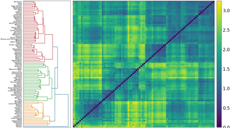
93 matrices D andR. Clustering based on Rreveals New York, New Jersey, Connecticut and Massachusetts as clear outliers. Indeed, these four U.S. states featured very high mortality rates in the early days of the pandemic in the United States. Clustering onDreveals far more insights. In the first instance, a cluster of Monaco, Liechtenstein, Iceland, Andorra and San Marino arises as clear outliers. We have removed these countries, all the five smallest in Europe, to obtain Figure 4.
Turning now to a close analysis of Figure 4, we observe the existence of three distinct clusters. The green cluster is almost exclusively composed of Northeastern U.S. states (Connecticut, Delaware, D.C., Maine, Maryland, Massachusetts, New Hamp-shire, New Jersey, New York, Pennsylvania, Rhode Island, and Vermont) and developed Western or Northern European coun-tries (Belgium, Denmark, Finland, France, Germany, Ireland,
As explored in Section II, many of these experienced simi-lar severe first waves, with most responding with lockdowns. These countries and states managed their progression from cases to deaths much more successfully in subsequent waves of COVID-19.
The orange cluster consists primarily of less developed Eu-ropean countries (Bulgaria, Croatia, Czech Republic, Greece, Hungary, Latvia, Lithuania, Poland, Slovakia and Slovenia) and select U.S. states such as Alaska and Kansas. These coun-tries and states all experienced less severe first waves, and more significant subsequent waves of the virus. Countries such as Croatia and Greece continued to attract travellers during the European summer,42which may have been an additional factor in spreading the virus. U.S. states such as Alaska and Kansas also both experienced less severe first waves in COVID-19, followed by extreme growth in both cases and deaths in
subsequent waves.
The red cluster is composed mostly of the remaining U.S. states and select European countries. Their case and death count have been steadily increasing over the entire period, for the most part.
IV. CONCLUSION
This paper introduces new methods to partition time se-ries and estimate offsets to quantify the changing mortality of COVID-19 over different waves of the pandemic. The method-ology is applied to European countries and U.S. states, both independently and in conjunction. Our methodology is flexible: different smoothing techniques, metrics between data, parame-ters in the algorithmic framework, and clustering methods can be used to study multivariate time series and identify changing mortality or other outcomes beyond this application.
Our analysis has refined the popular conception concerning the reduction of mortality during the second wave of COVID-19 in Europe.3We have shown significant variance in the mor-tality ratios (defined in Section II A), with European countries spanning a wide spectrum. For example, the Netherlands has reduced its mortality drastically, Germany has done so moder-ately, while Belarus’ mortality has slightly increased. Wealthy Western and Northern European countries, with the notable exceptions of Germany and Sweden, have reduced their mor-tality more than all U.S. states and the rest of Europe. Similar findings are observed with both one- and two-offset models. All these findings are reflected in the scatter plots of Figure 2, where a great difference in time-adjusted case and death data points is observed between the first wave and subsequent period. This considerable reduction in mortality has several explanations. In Europe, it has been surmised that the first wave’s case counts were drastically underestimated.16The first wave disproportionately affected the elderly,43while the sec-ond wave has largely affected young people,44 who have a much lower morbidity rate. It is also possible that the more socialized and equitable health systems of wealthy European countries have served their populations better than the United States,45resulting in higher mortality reductions than even the
(a) (b)
(c) (d)
FIG. 3: Hierarchical clustering on the one-offset and two-offset mortality pairs(M1,M2)and(N1,N2). European countries are clustered relative to(M1,M2)in (a) and(N1,N2)in (b). U.S. states are clustered relative to(M1,M2)in (c) and(N1,N2)in (d).
Moldova, Ukraine, Missouri, North Carolina and South Dakota do not have a subsequent period and so are excluded.
Northeastern U.S. states.
Despite the considerable variance in mortality reduction among European countries and the U.S. states, we have also shown broad similarity between the two groups. Hierarchical clustering on the one- and two- offset mortality pairs, shown in Figure 3, highlights a broadly similar structure among Eu-rope and the United States. Both groups, for the one- and two- offset models, consist of one predominant cluster and a smaller cluster. In each group, the smaller cluster consists of countries and states that experienced a severe first wave and were then able to substantially reduce their mortality during the subsequent period. These were predominantly wealthy Western European countries and Northeastern U.S. states. A consistent observation among both groups is that countries and states that experienced a severe first wave in cases reduced their mortality rate more effectively in subsequent waves. We then confirmed this in a statistical test for Europe, although it failed for the United States.
Our offset analysis also revealed insights regarding the time delay between cases and deaths in the first and subsequent waves. This finding was more consistent than the mortality reduction across both Europe and the United States. We found that the time offsetλ2between cases and deaths of the subse-quent period is systematically larger than that of the first wave, λ1. This is likely due to under-reporting in the first wave.
Val-ues ofλ1as small as zero indicate that during the first waves, the spike in deaths was happening at the exact same time as the spike in cases, suggesting that the cases were being observed too late, or not at all. Indeed, previous analysis46has showed that Spain had 2.27 times as many deaths on 03/28/2020 as the number of cases 16 days earlier. By the second wave, European countries and U.S. states were testing more consistently, soλ2 is likely a more accurate reflection of the time delay between cases and deaths.
Finally, Figure 4 analyzed all the European countries and U.S. states in conjunction, and again highlighted numerous similarities and differences between the groups. One cluster consisted of most wealthy Western European countries and Northeastern states alike, indicating their similar trajectories of both cases and deaths. Another cluster consists primarily of less affluent European countries such as Bulgaria, Croatia, Greece, Latvia and Poland. The third cluster consists primarily of the remaining U.S. states. In particular, while similarity exists between Western European countries and Northeastern U.S. states, there is no such close relationship between other European countries, such as less developed Eastern European countries, and other U.S. states outside the Northeast.
Overall, this paper introduces a new method for analyzing second wave mortality in a collection of epidemiological time series and provides new insights into the differing effects of
FIG. 4: Hierarchical clustering on the matrixD, defined in Section III. The five smallest European countries, which initially appeared as outliers, have been removed. The remaining dendrogram exhibits three characteristic clusters. One consists of predominantly wealthy Western European countries and Northeastern U.S. states. One consists predominantly of less affluent
European countries. The largest consists predominantly of the remaining U.S. states.
COVID-19 across Europe and the U.S. Midway through 2020, Europe had seen a substantial reduction of new case counts at the end of its first wave, and many European countries were praised for their handling of the virus. Few predicted the enormity of the second wave in Europe. Fortunately, wealthy Western countries, the Netherlands most of all, experienced a drastic drop in mortality. However, this is by no means uniform. Less developed countries are often underrepresented in media reports and their mortality is less visible in popular conception. As further waves carry the risk of widespread loss of life, each country must be aware of the potentially high human cost of COVID-19 and react swiftly to new waves of the pandemic.
DATA AVAILABILITY
The data that support the findings of this study are openly available at Refs. 47 and 48.
ACKNOWLEDGMENTS
The authors thank Kerry Chen for helpful comments and edits.
Appendix A: Turning point methodology
In this section, we provide more details for the identification of turning points of a new case time seriesx(t), in particular the first non-trivial troughT1. First, some smoothing of the time series is necessary due to irregularities in the data set, and discrepancies between different data sources. There are lower counts on the weekends, and some negative counts due to retroactive adjustments. A Savitzy-Golay filter ameliorates these issues by combining polynomial smoothing with a mov-ing average computation - this movmov-ing average eliminates all but a few small negative counts; we then replace these neg-ative counts with zero. This yields a smoothed time series ˆ
x(t)∈R≥0.Subsequently, we perform a two-step process to se-lect and then refine a non-empty setPof local maxima (peaks) andT of local minima (troughs). ThenT1is the first non-trivial element ofT.
Following Ref. 10, we apply a two-step algorithm to the smoothed time series ˆx(t). The first step produces an alternat-ing sequence of troughs and peaks, beginnalternat-ing with a trough at
t=0, where there are zero cases. The second step refines this sequence according to chosen conditions and parameters. The most important conditions to initially identify a peak or trough,
respectively, are the following: ˆ
x(t0) =max{xˆ(t): max(0,t0−l)≤t≤min(t0+l,T)}, (A1) ˆ
x(t0) =min{xˆ(t): max(0,t0−l)≤t≤min(t0+l,T)}, (A2) wherelis a parameter to be chosen. Following Ref. 10, we selectl=17, which accounts for the 14-day incubation period of the virus49and less testing on weekends. Defining peaks and troughs according to this definition alone has some flaws, such as the potential for two consecutive peaks.
Instead, we implement an inductive procedure to choose an alternating sequence of peaks and troughs. Supposet0is the last determined peak. We search in the periodt>t0for the first of two cases: if we find a timet1>t0that satisfies (A2) as well as a non-triviality condition ˆx(t1)<xˆ(t0), we addt1to the set of troughs and proceed from there. If we find a timet1>t0 that satisfies (A1) and ˆx(t0)≥xˆ(t1), we ignore this lower peak as redundant; if we find a timet1>t0that satisfies (A1) and
ˆ
x(t1)>xˆ(t0), we remove the peakt0, replace it witht1 and continue fromt1. A similar process applies from a trough att0.
At this point, the time series is assigned an alternating se-quence of troughs and peaks. However, some turning points are immaterial and should be removed. Lett1<t3be two peaks, necessarily separated by a trough. We select a param-eterδ =0.2, and if thepeak ratio, defined as xxˆˆ((tt3)
1) <δ, we
remove the peakt3. If two consecutive troughst2,t4remain, we removet2if ˆx(t2)>xˆ(t4), otherwise removet4. That is, if the second peak has size less thanδ of the first peak, we remove it.
Finally, we use the samelog-gradient function between timest1<t2, defined as
log-grad(t1,t2) =
log ˆx(t2)−log ˆx(t1)
t2−t1
. (A3) The numerator equals log(xˆ(t2)
ˆ
x(t1)), a "logarithmic rate of change."
Unlike the standard rate of change given by xˆ(t2)
ˆ
x(t1)−1, the
loga-rithmic change is symmetrically between(−∞,∞). Lett1,t2be adjacent turning points (one a trough, one a peak). We choose a parameterε=0.01; if
|log-grad(t1,t2)|<ε, (A4) that is, the average logarithmic change is less than 1%, we removet2from our sets of peaks and troughs. Ift2is not the final turning point, we also removet1.
We conclude with an alternating sequence of peaks and troughs, beginning with a trough att =0. We then simply defineT1to be the first trough aftert=0, if this exists. This marks the end of the first wave.
1M.-K. Looi, “Covid-19: Is a second wave hitting Europe?” BMJ , m4113
(2020).
2F. Walsh, “Coronavirus: Is it time to move on and get back to normal
life?”https://www.bbc.com/news/health-53951764, BBC, August 28, 2020.
3C. Cookson and J. Burn-Murdoch, “Why the second wave of Covid-19
appears to be less lethal,” https://www.ft.com/content/b3801b63-fbdb-433b-9a46-217405b1109f, Financial Times, October 21, 2020.
4S. McDonell, “Coronavirus: US and Australia close borders to Chinese
arrivals,”https://www.bbc.com/news/world-51338899, BBC, Febru-ary 2, 2020.
5J. McCurry, “Test, trace, contain: how South Korea flattened its
coro-navirus curve,” https://www.theguardian.com/world/2020/apr/ 23/test-trace-contain-how-south-korea-flattened-its-coronavirus-curve, The Guardian, U.S.April 23, 2020.
6A. McCann, N. Popovich, and J. Wu, “Italy’s virus shutdown came too
late. what happens now?”https://www.nytimes.com/interactive/ 2020/04/05/world/europe/italy-coronavirus-lockdown-reopen.html, The New York Times, U.S.April 5, 2020.
7G. Scally, B. Jacobson, and K. Abbasi, “The UK’s public health response to
covid-19,” BMJ , m1932 (2020).
8M. Iatiet al., “All 50 U.S. states have taken steps toward reopening in
time for Memorial Day weekend,”https://www.washingtonpost.com/ nation/2020/05/19/coronavirus-update-us, The Washington Post, May 20, 2020.
9R. Meyer and A. C. Madrigal, “A devastating new stage of
the pandemic,”https://www.theatlantic.com/science/archive/ 2020/06/second-coronavirus-surge-here/613522, the Atlantic, June 25, 2020.
10N. James and M. Menzies, “COVID-19 in the United States: Trajectories and
second surge behavior,” Chaos: An Interdisciplinary Journal of Nonlinear Science30, 091102 (2020).
11S. Griffin, “Covid-19: Second wave death rate is doubling fortnightly but is
lower and slower than in march,” BMJ , m4092 (2020).
12M. Wanget al., “Remdesivir and chloroquine effectively inhibit the recently
emerged novel coronavirus (2019-nCoV) in vitro,” Cell Research30, 269– 271 (2020).
13E. M. Bloch, “Convalescent plasma to treat COVID-19,” Blood136, 654–
655 (2020).
14X. Xu et al., “Effective treatment of severe COVID-19 patients with
tocilizumab,” Proceedings of the National Academy of Sciences117, 10970– 10975 (2020).
15B. Caoet al., “A trial of Lopinavir-Ritonavir in adults hospitalized with
se-vere Covid-19,” New England Journal of Medicine382, 1787–1799 (2020).
16R. Liet al., “Substantial undocumented infection facilitates the rapid
dis-semination of novel coronavirus (SARS-CoV-2),” Science368, 489–493 (2020).
17H. W. Hethcote, “The mathematics of infectious diseases,” SIAM Review
42, 599–653 (2000).
18G. Chowell, L. Sattenspiel, S. Bansal, and C. Viboud, “Mathematical models
to characterize early epidemic growth: A review,” Physics of Life Reviews 18, 66–97 (2016).
19S. K. Biswas, U. Ghosh, and S. Sarkar, “Mathematical model of Zika virus
dynamics with vector control and sensitivity analysis,” Infectious Disease Modelling5, 23–41 (2020).
20R. E. Morrison and A. Cunha, “Embedded model discrepancy: A case study
of Zika modeling,” Chaos: An Interdisciplinary Journal of Nonlinear Science 30, 051103 (2020).
21S. Funk, A. Camacho, A. J. Kucharski, R. M. Eggo, and W. J. Edmunds,
“Real-time forecasting of infectious disease dynamics with a stochastic semi-mechanistic model,” Epidemics22, 56–61 (2018).
22A. Mhlanga, “Dynamical analysis and control strategies in modelling
ebola virus disease,” Advances in Difference Equations 2019 (2019), 10.1186/s13662-019-2392-x.
23C. Manchein, E. L. Brugnago, R. M. da Silva, C. F. O. Mendes, and M. W.
Beims, “Strong correlations between power-law growth of COVID-19 in four continents and the inefficiency of soft quarantine strategies,” Chaos: An Interdisciplinary Journal of Nonlinear Science30, 041102 (2020).
24J. A. T. Machado and A. M. Lopes, “Rare and extreme events: the case of
COVID-19 pandemic,” Nonlinear Dynamics (2020), 10.1007/s11071-020-05680-w.
25N. James and M. Menzies, “Cluster-based dual evolution for multivariate
time series: Analyzing COVID-19,” Chaos: An Interdisciplinary Journal of Nonlinear Science30, 061108 (2020).
(2020).
27A. Vazquez, “Polynomial growth in branching processes with diverging
reproductive number,” Physical Review Letters96(2006), 10.1103/phys-revlett.96.038702.
28R. Moeckel and B. Murray, “Measuring the distance between time series,”
Physica D: Nonlinear Phenomena102, 187–194 (1997).
29G. J. Székely, M. L. Rizzo, and N. K. Bakirov, “Measuring and testing
dependence by correlation of distances,” The Annals of Statistics35, 2769– 2794 (2007).
30C. F. Mendes and M. W. Beims, “Distance correlation detecting Lyapunov
instabilities, noise-induced escape times and mixing,” Physica A: Statistical Mechanics and its Applications512, 721–730 (2018).
31C. F. O. Mendes, R. M. da Silva, and M. W. Beims, “Decay of the distance
autocorrelation and Lyapunov exponents,” Physical Review E99(2019), 10.1103/physreve.99.062206.
32K. Shang, B. Yang, J. M. Moore, Q. Ji, and M. Small, “Growing networks
with communities: A distributive link model,” Chaos: An Interdisciplinary Journal of Nonlinear Science30, 041101 (2020).
33A. Karaivanov, “A social network model of COVID-19,” PLOS ONE15,
e0240878 (2020).
34A.-M. Madoreet al., “Contribution of hierarchical clustering techniques
to the modeling of the geographic distribution of genetic polymorphisms associated with chronic inflammatory diseases in the Québec population,” Public Health Genomics10, 218–226 (2007).
35M. Kretzschmar and R. T. Mikolajczyk, “Contact profiles in eight European
countries and implications for modelling the spread of airborne infectious diseases,” PLoS ONE4, e5931 (2009).
36H. Alashwal, M. E. Halaby, J. J. Crouse, A. Abdalla, and A. A. Moustafa,
“The application of unsupervised clustering methods to Alzheimer’s dis-ease,” Frontiers in Computational Neuroscience13(2019), 10.3389/fn-com.2019.00031.
37H. Muradi, A. Bustamam, and D. Lestari, “Application of hierarchical
clus-tering ordered partitioning and collapsing hybrid in Ebola virus phylogenetic analysis,” in2015 International Conference on Advanced Computer Science
R. Rizzi, P. Mahata, L. Mathieson, and P. Moscato, “Hierarchical clustering using the arithmetic-harmonic cut: Complexity and experiments,” PLoS ONE5, e14067 (2010).
39“Worldodometer,”
https://www.worldometers.info/geography/ how-many-countries-in-europe/ (2020), accessed November 25, 2020.
40“Our World in Data,” https://ourworldindata.org/covid-data-switch-jhu(2020), accessed November 25, 2020.
41D. Avis, D. Bremner, and R. Seidel, “How good are convex hull algorithms?”
Computational Geometry7, 265–301 (1997).
42F. Campana, “How greece is rethinking its once bustling tourism industry,” https://www.nationalgeographic.com/travel/2020/09/how-greece-is-coping-without-tourism-due-to-covid/, National Geographic, September 22, 2020.
43E. Kontopantelis, M. A. Mamas, J. Deanfield, M. Asaria, and T. Doran,
“Excess mortality in england and wales during the first wave of the COVID-19 pandemic,” Journal of Epidemiology and Community Health , jech–2020– 214764 (2020).
44A. Aleta and Y. Moreno, “Age differential analysis of COVID-19 second
wave in europe reveals highest incidence among young adults,” medRxiv (2020), 10.1101/2020.11.11.20230177.
45L. A. Burke and A. M. Ryan, “The complex relationship between cost and
quality in US health care,” AMA Journal of Ethics16, 124–130 (2014).
46N. James and M. Menzies, “Cluster-based dual evolution for multivariate
time series: Analyzing COVID-19,” Chaos: An Interdisciplinary Journal of Nonlinear Science30, 061108 (2020).
47“Our World in Data,” https://ourworldindata.org/coronavirus-source-data(2020), accessed November 25, 2020.
48“Coronavirus (Covid-19) data in the United States,”https://github. com/nytimes/covid-19-data, The New York Times, Accessed Novem-ber 25, 2020.
49S. A. Laueret al., “The incubation period of Coronavirus disease 2019
(COVID-19) from publicly reported confirmed cases: Estimation and appli-cation,” Annals of Internal Medicine172, 577–582 (2020).