GMM Estimation of Autoregressive Roots Near Unity with Panel Data
By
Peter C.B. Phillips and Hyungsik Roger Moon
January 2003
COWLES FOUNDATION DISCUSSION PAPER NO. 1390
COWLES FOUNDATION FOR RESEARCH IN ECONOMICS
YALE UNIVERSITY
Box 208281
New Haven, Connecticut 06520-8281
GMM Estimation of Autoregressive Roots
Near Unity with Panel Data
∗
Hyungsik Roger Moon
Department of Economics
University of Southern California
&
Peter C.B. Phillips
Cowles Foundation, Yale University
University of Auckland & University of York
November 2002
Abstract
This paper investigates a generalized method of moments (GMM) approach to the estimation of autoregressive roots near unity with panel data and incidental deterministic trends. Such models arise in empirical econometric studies of Þrm size and in dynamic panel data modeling with weak instruments. The two moment conditions in the GMM approach are obtained by constructing bias corrections to the score functions under OLS and GLS detrending, respectively. It is shown that the moment condition under GLS detrending corresponds to taking the projected score on the Bhattacharya basis, linking the approach to recent work on projected score methods for models with inÞnite numbers of nuisance parameters (Waterman and Lindsay, 1998). Assuming that the localizing parameter takes a nonpositive value, we establish consistency of the GMM estimator andÞnd its limiting distribution. A notable newÞnding is that the GMM estimator has convergence rate n1/6, slower than√n,when the true localizing parameter is zero (i.e., when there is a panel unit root) and the deterministic trends in the panel are linear. These results, which rely on boundary point asymptotics, point to the continued difficulty of distinguishing unit roots from local alternatives, even when there is an inÞnity of additional data. JEL ClassiÞcation: C22 & C23
Keywords and Phrases: Bias, boundary point asymptotics, GMM estimation, local to unity, moment conditions, nuisance parameters, panel data, pooled regression, projected score.
∗The authors are grateful to J. Horowitz and two referees for comments on earlier versions, to J.
Owens for excellent research assistance, to J. Hahn and D. Bowman for helpful discussions, and to R.
Waterman for sharing with us his recent joint papers with B. Lindsay. Moon thanks the Academic
Research Committee of UCSB and the Faculty Development Awards of USC for research support and Phillips thanks the NSF for research support under NSFs SBR 97-30295 & SES 0092509.
1
Introduction
Recent years have seen the introduction of several important panel data sets where the cross sectional dimension (n)and the time series dimension (T)are comparable in magni-tude. Some of these panel data sets, like the Penn World Tables, involve time series that are manifestly nonstationary and have persistent or slowly decaying serial correlations. These features distinguish the new data from the characteristics that are conventionally assumed in the analysis of panel data whereT is very small andnis very large.
Since the early 1990’s, there has been ongoing theoretical and applied research on panels whose time series components are nonstationary or persistent. For large n and
ÞxedT panels, see Hahn et al (2001) and Kruiniger (2000). For largen and T panels allowing for nonstationarity in the data over time, the theoretical research includes the study of asymptotically unbiased estimation of the dynamic panel model (e.g.,Hahn and Kuersteiner, 2000), panel unit root tests (e.g.,Quah, 1994, Levin and Lin, 1993, Imet al.,
1996, Maddala and Wu, 1997, and Choi, 1999), panel cointegration tests (e.g.,Pedroni, 1999, Binder et al., 1999), and the development of linear regression theories for panel estimators under nonstationarity (e.g.,Pesaran and Smith, 1995, and Phillips and Moon, 1999). Applied research includes tests of growth convergence theories (Bernard and Jones, 1996), purchasing power parity relations (MacDonald, 1996, Oh, 1996, Pedroni, 1996, Wu, 1996, and Wu, 1997), and studies of the international links between savings and investment (Coakleyet al., 1996 and Moon and Phillips, 1998).
Two recent papers by the authors (Moon and Phillips, 1999 & 2000) study panel regression models that allow for both deterministic trends and stochastic trends with roots local to unity. As we discuss in Section 2 of the present paper, such models are important empirically in studying Gibrat’s law and they have received attention recently in the weak instrument literature. When the deterministic trends in nonstationary panel data are heterogeneous across individuals, Moon and Phillips (1999) show that the maximum likelihood estimator (MLE) of the local to unity parameter in the stochastic trend is inconsistent. They call this phenomenon, which arises because of the presence of an inÞnite number of nuisance parameters, an incidental trend problem because it is analogous to the well-known incidental parameter problem in dynamic panels when T is Þxed1. To solve the incidental trend problem, Moon and Phillips (2000) propose various methods, including an iterative ordinary least squares (OLS) procedure and a double bias corrected estimator, and establish limit theories for these consistent estimators that can be used for statistical inference about the localizing parameter.
As a continuation of the two studies just mentioned, the present paper investigates a generalized method of moments (GMM) estimator of autoregressive roots near unity with panel data. We establish two moment conditions that form the basis for inference. The
Þrst moment condition is obtained by adjusting for the bias of the score function after con-ventional OLS detrending. The second moment condition is constructed by adjusting for the bias of the score function following quasi-difference (QD) detrending. Interestingly, the second moment condition is shown to correspond to the Gaussian projected score, where the projection is taken on the so-called Bhattacharya basis that has been studied recently in the conventional incidental parameter problem by Waterman and Lindsay (1996, 1998) and Hahn and Kuersteiner (2000). Unlike the conventional moment conditions used in estimating dynamic panel data models, these moment conditions do not suffer the weak instrument problem that is discussed, for example, in Kruiniger (2000) and Hahn et al.
(2001).
Consistency of the GMM estimator is proved under the assumption that the local-izing parameter takes a nonpositive value. This condition is not too restrictive because 1Lancaster(2000) provides a recent general survey of the incidental parameter problem in econometrics.
most econometric models consider non-explosive autoregressive regression models. Nev-ertheless, the restriction does matter in deriving the limiting distribution of the estimator because it is possible that the true parameter lies on the boundary of the parameter set. The most interesting case is, of course, the pure unit root case where the true localizing parameter is zero. In this case, in establishing the limiting distribution we cannot use the conventional approach that approximates the Þrst order condition because the true parameter could be on the boundary of the parameter set. To avoid this difficulty, we use the approach that takes a quadratic approximation of the nonlinear objective function and optimize it on the parameter set (c.f. Andrews, 1999, for some recent developments of estimation and inference in boundary problems).
One of the most interestingÞndings in the present paper is that the GMM estimator has slower convergence rate than√nwhen the time series components in the panel have unit roots (i.e., the true localizing parameter is zero), and the deterministic trends are linear. In this case the convergence rate is actually O(n1/6) rather than O(√n). This
slow convergence rate arises because of lack of information in the moment conditions when there is a unit root, i.e., at the pointc= 0in the space of the localizing parameter. It points to the continued difficulty of distinguishing unit roots from local alternatives in the presence of heterogeneous deterministic trends even when there is an inÞnity of additional data from a cross section.
The paper is organized as follows. Section 2 lays out the model and gives the basic assumptions that are maintained throughout the paper. We also discuss the empirical relevance of the model and the conventional moment conditions used in dynamic panels models of this type. In section 3 we introduce two new moment conditions and prove that the second of these moment conditions corresponds to a Gaussian projected score on the Bhattacharya basis. In Section 4 we establish consistency of the GMM estimator and obtain the limiting distributions of the GMM estimator when the true parameter is less than zero and equal to zero. The appendix contains technical derivations and proofs of the results in the main text.
2
Persistent Dynamic Panels
2.1
The Model and Assumptions
We study panel data that may show characteristics of time trends and persistent tem-poral shocks and whose dimension is large in both cross section (n)and time series (T)
dimensions. To model such data, we extend the conventional dynamic panel model by taking the components formulation
zit=β0igpt+yit, (1)
where gpt =
¡
t, t2, ..., tp¢0, the coefficients β
i are p−vectors that could be random, and
the residualsyitfollow
yit=ρyit−1+εit
with a common autoregressive coefficient ρthat is close to one deÞned in (4) below. Let
yi0 = zi0 be the panel observations at the initial time period. In (1), the Þrst term β0igpt represents deterministic trends in the data, omitting an intercept because this is
not consistently estimable from time series data whenyitis near integrated (e.g.,Phillips
and Lee, 1996) and can be incorporated in the initial condition yi0. Assuming that the
or Þxed effects in the panel. Sinceρ is in the vicinity of unity, the componentsyit have
stochastic trends with persistent innovationsεit.
The components model (1) can also be written in the more familiar format of an augmented regression form as
zit=ρzit−1+δi+γ0igpt+εit, (2) where δi = ρβ0iιp, ιp=− ³ −1,(−1)2, ...,(−1)p´0, γ0i = β0iΥ(ρ), Υ(ρ) is a (p×p) matrix depending onρ.
For example, when p= 1, the deterministic panel trends are linear and the augmented model (2)is
zit=ρβi+ (1−ρ)βit+ρzit−1+εit. (3)
This linear trend model (3) is an extended version of the standard model for dynamic panels in which the individual effects are the incidental trends ρβi+ (1−ρ)βit and the autoregressive parameter is assumed to be close to one.2
The augmented format(2)has the drawback that linear regression leads to inefficient trend elimination, but the advantage that the detrended data is invariant to the trend parameters in(2).In the next section, we use the augmented formation(2)to deÞne the
Þrst moment condition, and the component model(1)for the second moment condition. To enable a rigorous development whenρ is close to one, we take the speciÞc near unity formulation,
ρ= 1 + c
T, (4)
or equivalently,
T(ρ−1) =c,
in which the standardized deviation of the coefficient ρfrom unity remains constant (c).
In this case, the stochastic trendsyitare near integrated and they are characterized by the
parametercinstead of the autoregressive coefficientρ. The time series properties of the near integrated process yit are well known from the nonstationary time series literature
(e.g.,Phillips, 1987, and Stock, 1994). Recently, Hahnel al.(2001) and Kruiniger (2000) use the related speciÞcation ρ= 1 + nc to model an autoregressive coefficient near unity in a panel with large nand ÞxedT.
In a conventional time series autoregression (AR), the probabilistic features (and the asymptotics) are discontinuous with respect to the AR coefficient as it passes through unity. When|ρ|<1, the process is stationary, reverts to its mean, converges to a steady state, and has no stochastic trend, whereas whenρ= 1, the process is nonstationary, not mean-reverting, and contains stochastic trends. Models with near unit roots as in(4)have probabilistic features that are continuous with respect to parameterc,while still retaining some of the implications of the three different cases: ρ< 1(c <0), ρ= 1 (c= 0), and
ρ > 1 (c >0). More speciÞcally, a direct calculation shows that V ar(yit) increases at
the ratet,regardless of the sign of the parameterc.Thus,yitis nonstationary and has a
2For other examples of incidental trend models, see Section 11.2.1 of Wooldridge (2001) and the
stochastic trend regardless of the sign of the parameter c.On the other hand, when for
t= [T r]with0< r≤1,it is well known that
yit √ T ⇒Jc(r) asT → ∞, (5) whereJc(r) = Rr 0 e
c(r−s)dW(s)is the Ornstein-Uhlenbeck process, andW(s)is a
Brown-ian motion (e.g.,Phillips, 1987).So, the marginal asymptotic distribution of the standard-ized process√yit
T is continuous inc.Also, whenc <0,the limit processJc(r)is stationary
and mean reverting, while for c = 0, the limit process is Brownian motion. Thus, the standardized process √yit
T preserve some of the probabilistic implications implied by the
conventional AR(1) model for|ρ|<1andρ= 1.One beneÞt of the continuity property is that it is possible to produce conÞdence intervals for the AR coefficientρfrom estimates ofc(Stock, 1991) even though consistent estimation ofcfrom time series observations is not possible. In this paper we use notationc0to denote the true coefficient forc.
In later sections of the paper, as part of the asymptotic development, we need to verify some properties of complicated nonlinear functions of cthat depend on the trend
gpt.These functions are so complicated that it is very difficult to establish analytic results
under the general polynomial trend set up with gpt = (t, ..., tp)0. Instead, we rely on
numerical methods for this part of the analysis. To assist the analytic development, we restrict our attention to the following two cases: (i) g1t =t and (ii)g2t =
¡
t, t2¢0. This
restriction is hardly restrictive in practice because the linear and quadratic trends are the most widely used in empirical applications.The set up is formalized as follows:
Assumption 1 (Trend Formulation)
The polynomial trend in model(1) is either (i) g1t=t or (ii)g2t=¡t, t2¢0.
Assumption 2 (Initial Condition) The initial observations zi0 = yi0 are independent across iwithsupiEy4i0<∞.
Assumption 3 (Error Condition) The error terms εit∼iid
¡
0,σ2¢ acrossi and t with Eε4
it<∞andεit are independent of yi0 for alli. Assumption 4 (Parameter Set)
(a) The localizing parameter ctakes a value in a compact subset C= [ ¯c , 0 ] ⊂ R,
where ¯c <0.
(b) The true localizing parameterc0 is in the set C0= (¯c, 0 ].
Assumption 4(a) restricts the parameter setC= [¯c , 0] to be non-positive. This re-striction is made because in most econometric applications, the cases |ρ| <1andρ= 0
are of most interest. When the true parameter c0 = 0, the model becomes nonstandard
in the sense that the true parameter is on the boundary of the parameter set. Section 4.3 explores the implications of the boundary point aspect of this case.
The practical implication of the restriction ofc0toC= [¯c ,0]is of some interest. One
of the advantages of pooling is that consistent estimation of c0 is achievable with panel
data while it is not with a single time series. Take the case where the true valueρ0= 1+c0 T
lies in the interior of the compact interval [1 + T¯c,1] for some c <¯ 0. Theorem 3 below shows that the GMM estimatorˆcis consistent forc0 and has a limit normal distribution
√
n(ˆc−c0)→dZ. The corresponding autoregressive coefficient estimate isˆρ= 1 +Tˆc and
√
nT(ˆρ−ρ0)→d Z.So, panel pooling affects the ‘usual asymptotic distribution’ of the
autoregressive coefficient in near integrated models. The distribution is normal and lives in a shrunken neighbourhood within the compact set[1 +T¯c,1].In effect,ˆρis distributed
in an O³√1
n
´
neighbourhood of the true valueρ0 ∈ [1 + ¯c
T,1]. The main thrust of the
present work is to put panel pooling to good effect, so that we get this increased precision about the value of ρ0 even when it is already in the locality of unity. To the extent that many economic time series are near integrated but also may have idioscyncratic deterministic trend components, this process increases precision in estimation, conÞdence interval construction and local discriminatory power at unity for ρ0 (where it increases fromO¡T−1¢to O³T−1n−1
6 ´
- see section 4.3), but also near unity (where it increases fromO¡T−1¢to O³T−1n−12
´
- see section 4.2).
Assumption 5 (n, T → ∞)with loglogTn <2 +O³log1T´.
Assumption 5 restricts the relative size of the cross-section and temporal dimensions in the panel in the asymptotic theory. It is assumed thatnincreases at a lesser speed than
T2 asT → ∞. So if n=Tα thenα<2, thereby allowing for panels in whichnand T
are of comparable size satisfying n
T →κ,0<κ<∞,as in Hahn and Kuersteiner, 2000),
and some panels where the size of the cross section dominates the time series count, i.e.,
n
T → ∞. This assumption is required for the derivation of the limit distribution of the
estimator ofcin Section 4. Consistency of the estimator does not require this restriction.
2.2
Discussion of the Model
2.2.1 Empirical Relevance in Modeling Firm Size
In the empirical industrial organization literature onÞrm size, dynamic panel models have been used widely to describe Þrm growth in terms of a simple formulation that follows the spirit of Gibrat’s law of proportional effect (Gibrat, 1931). Gibrat’s law states that the expected value of the increment in a Þrm’s size each time period is proportional to the current size of theÞrm. LetZit denote the size ofÞrmiat time tandeitdenote the
(stochastic) proportionate rate of growth ofÞrmibetween timetandt−1.Then Gibrat’s law is formalized as
Zit−Zit−1=Zit−1eit.
(e.g., Steindle, 1965, and Sutton, 1997). Let zit = logZit and, using the approximation
log(1 +a)≈afor smalla,we may write the proportional law in autoregressive form as
zit=zit−1+eit, (6)
which McCloughan (1995) calls Gibrat’s process — a law in which the growth rate of a
Þrm is independent of its initial size. Wheneit∼iid
¡
µ,σ2
e
¢
, setεit=eit−µ, and then
we may rewrite Gibrat’s process(6)in the component form
zit = µt+yit, (7)
yit = yit−1+εit,
which is a special case of model (1). The panel model (1) (or (2)) can therefore be interpreted as a generalized version of Gibrat’s process when applied toÞrm growth data. To motivate (1), we now discuss more detailed features of the model in the context of this application and indicate how we can explain in terms of this model (1) some empirical
First we consider several well known implications of Gibrat’s law. For T large, by virtue of the functional central limit theorem applied to T−1/2z
it in (6), the
distribu-tion of Þrm size Zit is approximately lognormal and therefore skewed. Evidence
sup-porting lognormality and skewness ofÞrm size distributions has been reported in many past empirical papers. The more recent literature argues thatÞrm size distributions do not follow a ‘typical’ distributional shape but nevertheless have skewness as their cen-tral characteristic (e.g., Sutton, 1997, and Schmalensee, 1989). Next, observing that
∆V ar(zit) :=V ar(zit)−V ar(zit−1) =σ2in Gibrat’s process (7),Prais (1976) and more
recently McCloughan (1995) claimed that the proportionate model implies that size in-equalities between Þrms will increase at a constant rate, and the rate of concentration will be greater the higher the variance of the growth distribution,σ2.For this reason, Mc-Cloughan (1995) calls∆V ar(zit) =σ2Gibrat’s effect. For other implications of Gibrat’s
law, see Lucas (1978) and Sutton (1997).
Over the last two decades, many studies have found empirical violations of Gibrat’s law. These are reviewed and classiÞed in McCloughan (1995). For example, Evans (1987) found through a cross-sectional analysis that Þrm growth decreases with Þrm age and
Þrm size, which is claimed to be consistent with the prediction made by the theory in Jovanovic (1982). More recently, Hall and Mairesse (2000) investigated the time series properties of several variables in Þrm-level panel data that are related to the growth of
Þrms. One of theirÞndings was that the growth rates of these variables vary widely across
Þrms. Another was that the sample serial correlations typically decay very slowly. In what follows, we compare the implications of the panel model (1) with those of Gibrat’s process and consider possible explanations, in terms of (1), of the empirical violations of the law.
(i) According to (1)and (4), the stochastic shock in the logarithm ofÞrm size is nearly integrated and involves the parameterc.As discussed earlier, forT large this formulation ensures that the distribution of Þrm size is asymptotically lognormal, as indicated by Gibrat’s law3. Also, since the autoregressive coefficient ρ is close to unity for large T, the serial correlations ofzitwill not decay. These properties coincide with what Hall and
Mairesse (2000) observe in theirÞrm panel data.
(ii) Since the random growth rate process is∆zit=δi+γ0igpt+Tczit−1+εit,we have
∂∆zit
∂zit−1 = c
T <0ifc <0.Thus,Þrm growth decreases asÞrm size increases, giving the size
effect.
(iii) If the deterministic trends are quadratic and the coefficient of the quadratic
coef-Þcient is negative, we have the age effect because ∂E(∆zit)
∂t = 2βi2<0whenzi0=yi0= 0.
(iv) A simple calculation shows that
V ar(zit) =σ2 ³ 1 +ρ2+...+ρ2(t−1)´∼σ2 t−1 X s=0 exp³2cs T ´ (8) whenyi0is nonrandom. So,
∆V ar(zit)'σ2exp µ 2ct−1 T ¶ . (9)
3In empirical studies, a commonly used model for representing a generalized Gibrat process is the
conventional AR(1) model
zit=µ+ρzit−1+eit,
e.g., McCloughan, 1995, and Hall and Mairesse, 2000. In this case, when−1<ρ<1,the size distribution depends on the distribution of the error eit and skewess of the size distribution is not guaranteed. By
Equations (8) and (9) indicate that inequalities inÞrm growth grow over time and the rate of change in the inequality depends on the value of the growth parameterc.
(v) Model (2) introduces individual speciÞc effects through the trend coefficients βi
and the initial conditions zi0. These effects may explain certain heterogeneous factors
such as the x-inefficiency of someÞrms.
In view of these characteristics, the panel model (2) helps to bridge the gap between the pure form of Gibrat’s law and the empirical evidence indicating certain systematic violations of the law. In addition, consistent estimation of the systematic growth parame-tercmakes it possible to measure the size effect and changes in growth inequality orÞrm concentration.
2.2.2 Conventional Moment Conditions and Weak Instruments
In recent years, one of the most widely used methods of estimating dynamic panel regres-sion models withÞxed effects, such as
zit= (1−ρ)βi+ρzit−1+εit,
is to utilize the moment conditions implied by the assumptions imposed on the model. (For details and references, see the recent survey by Arellano and Honore, 2000). Among these moment conditions4, the moment restrictions known as the basic moment conditions, viz.,
E(zis∆εit) = 0fors= 0, ..., t−2, (10)
are the most widely applied. This section considers the properties of the basic form of moment conditions implied by the model (1).
For simplicity, we consider only the linear trend case, i.e.,
zit=ρβi+ (1−ρ)βit+ρzit−1+εit.
Due to the presence of the incidental trends, instead of (10)the basic moment conditions in the model 1 are
E¡zis∆2εit¢= 0 fors= 0, ..., t−3, (11)
which provide the orthogonality conditions in an instrumental variable regression of
∆2zit=ρ∆2zit−1+∆2εit, (12)
with instrumental variableszis, s= 0, ..., t−3.Notice from (12) that the basic moment
conditions (11)are linear in the parameterρ.To evaluate the orthogonality conditions in (11)in terms of their information content, we calculate theÞrst derivative of the moments with respect to the parameterρ.Then,
∂E¡zis¡∆2zit−ρ∆2zit−1¢¢
∂ρ =E
¡
zis∆2zit−1¢,s= 0, ..., t−3,
which is the covariance between the instrumental variablezis and regressor in (12).
First, when ρ = 1, as is well known in the conventional dynamic panel model, the information content of the basic moment conditions is zero becauseE¡zis∆2zit−1
¢
= 0
4Other types of moment conditions used in conventional dynamic panel models are derived under
extra assumptions on the initial conditions, the Þxed effect parameter, and the covariance stationarity restrictions.
fors= 0, ..., t−3, and so the instruments are not correlated with the regressors of (12). In this case, the parameterρis not identiÞable from the basic moment conditions.
Whenρ= 1 + c
T withc <0,a direct calculation shows that
E¡zis∆2zit−1 ¢ =³c T ´2 E(βis+yis) (2βi+yt−3)∼O µ 1 √ T ¶ .
This implies that if the coefficient is near unity as in (4)and the time dimension is large, the information in the basic moment conditions is small, and the instrumentszis become
weak5. In consequence, GMM estimation involving only conventional moment conditions cannot estimate the model consistently. This has become an issue of some importance in empirical studies of dynamic panel regression.
We therefore proceed to consider a different approach that augments the information content of the basic moment conditions. This approach arises from a consideration of the incidental trends problem, which we now discuss.
2.2.3 Incidental Trends Problem
Two recent papers by the authors (Moon and Phillips, 1999 & 2000) Þnd that an in-cidental trend problem arises in estimating the local to unity parameter c in the panel regression model (1) or (2) where inÞnite number of nuisance parameters are present. Moon and Phillips (1999) show that the score of the (pseudo) likelihood that concentrates out the incidental trend parametersβi are biased (even in the limit). In consequence, the maximum likelihood estimator (MLE) ofcin(1)is inconsistent. Also, according to Moon and Phillips (2000), when the incidental trend parametersβi are eliminated by ordinary least squares (OLS) projection, the normal equation of the pooled OLS estimator is biased as well (even in the limit) due to the correlation between the OLS detrended error term and the OLS detrended regressor. It follows that the pooled OLS estimator ofcobtained from OLS detrended data is also biased.
3
Moment Conditions
We now propose an estimation procedure that eliminates the effects of the incidental trend problem. The approach involves GMM and minimizes a distance criterion based on a vector of sample moment functions. The moment conditions are designed to have a limit that will identify the true localizing parameterc0 even in the presence of the incidental
trend coefficientsβi.
The principle we use for contructing moment conditions with this property is to adjust for the bias that arises in the usual score functions, the latter being explained in Moon and Phillips (1999, 2000). The adjustments are based on formulae from the explicit computation of the bias functions. The next subsections explain these constructions in detail.6
5When T is Þnite andnis large, Hahn et al (2001) and Kruiniger (2000) investigate similar weak
intrument effects in the conventional dynamic panel regression model with near unit root speciÞcations
ρ= 1 +nc.
6The principle employed can be applied to any biased score function for transformed data that is
invariant to the incidental trend coefficients. A referee suggested such a biased score function that leads to an alternative moment condition that turns out to be closely related to theÞrst moment condition described below. In view of this similarity and space constraints, we do not investigate this alternative moment condition here.
3.1
The First Moment Condition
The following notation is deÞned to assist with the analysis of the trend function asymp-totics and it will be used throughout the rest of the paper. Let
˜ γi = (δi,γ0i)0, ˜ gpt = ¡1, gpt0 ¢0 , gp(r) = (r, ..., rp)0 withr∈[0,1], g˜p(r) =¡1, gp(r)0¢0, Gp,T = ¡ gp01, ..., g0pT¢0, Gp,T,−1= ¡ gp00, ..., gpT0 −1¢0, G˜p,T = ¡ ˜ g0p1, ...,˜g0pT¢0, ˜ Mp,T = IT−G˜p,T ³ ˜ G0p,TG˜p,T ´−1 ˜ G0p,T, Dp,T = diag(T, ..., Tp), D˜p,T =diag(1, Dp,T), hpT(t, s) = gpt0 Dp,T−1 Ã 1 T T X t=1 D−p,T1gptg0ptDp,T−1 !−1 Dp,T−1gps, ˜ hpT(t, s) = g˜pt0 D˜p,T−1 Ã 1 T T X t=1 ˜ D−p,T1g˜pt˜g0ptD˜p,T−1 !−1 ˜ Dp,T−1g˜ps, hp(r, s) = gp0 (r) µZ 1 0 gp(r)gp(r)0dr ¶−1 gp(s), ˜ hp(r, s) = g˜p0 (r) µZ 1 0 ˜ gp(r) ˜gp(r)0dr ¶−1 ˜ gp(s). Writezi= (zi1, ..., ziT)0, zi,−1= (zi0, ..., ziT−1)0,andεi= (εi1, ...,εiT)0. DeÞne z ˜i = ˜Mp,Tzi, ε ˜i = ˜Mp,Tεi, z ˜i,−1 = ˜Mp,Tzi,−1.
Then, it is straightforward to show that
z ˜i =y ˜i andz ˜i,−1 =y ˜i,−1 , where y ˜i = ˜Mp,Tyi, y ˜i,−1 = ˜Mp,Tyi,−1, yi= (y1, ..., yT)0,andyi,−1= (y0, ..., yT−1)0.Let µ z ˜i,−1 ¶ t =zit−1− 1 T T X s=1 ˜ hpT(t, s)zis−1 be thetthelement ofz ˜i,−1.
One straightforward procedure of estimatingc0 (equivalentlyρ0= 1 +cT0)is to
elim-inate the unknown trends δi+γ0igpt by taking OLS regression residuals and then apply
pooled least squares with an appropriate bias correction for the serial correlation ofεit.
We call this method iterative OLS. However, as noted in Moon and Phillips (2000), this iterative OLS procedure yields an inconsistent estimator of c0 due to a
nondegenerat-ing asymptotic bias between the detrended regressor and the detrended error term. The
Þrst moment condition is obtained simply by subtraction of this asymptotic bias term in iterative OLS from the normal equation for the OLS detrended data.
More speciÞcally, write the model(2)in vector notation as
zi=ρ0zi,−1+ ˜Gp,Tγ˜i+εi, ρ0= 1 + c0
T. (13)
ApplyingM˜pT to both sides, we have
z ˜i =ρ0z ˜i,−1 +ε ˜i , (14) wherez ˜i , z ˜i,−1 ,andε ˜i
are OLS detrended versions ofzi, zi,−1,andεi,respectively. In
gen-eral, the detrended regressor vectorz
˜i,−1and the detrended error vectorε˜i are correlated
and theÞrst moment condition is found by correcting for the bias due to the correlation betweenz
˜i,−1
and ε
˜i
.
Before we deÞne the Þrst moment condition, we discuss the estimation of the error varianceσ2.Letˆρbe the pooled OLS estimator of(14),
ˆ ρ= Pn i=1z˜0 i z ˜i,−1 Pn i=1z˜0 i,−1 z ˜i,−1 , andˆε ˜i
be the OLS residual of(14),ˆε
˜i =z ˜i− ˆ ρz ˜i,−1 .The estimator of σ2 is ˆ σ2= 1 nT n X i=1 ˆ ε ˜ 0 i ˆ ε ˜i . (15)
TheÞrst moment condition formula is deÞned as
m1,iT(c) = 1 T µ z ˜i− ³ 1 + c T ´ z ˜i,−1 ¶0 z ˜i,−1 + ˆσ2ωpT(c) (16) = 1 Tε˜ 0 i y ˜i,−1 −(c−c0) 1 T2y ˜ 0 i,−1 y ˜i,−1 + ˆσ2ωpT(c) = 1 T T X t=1 εityi,t−1− 1 T2 T X t=1 T X s=1 εityi,s−1˜hpT(t, s)−(c−c0) 1 T2 T X t=1 à y ˜i,−1 !2 t + ˆσ2ωpT(c), where ωpT(c) = 1 T2 T X t=2 t−1 X s=1 ·³ 1 + c T ´T¸t−Ts−1 ˜ hpT(t, s), andε ˜it and(y ˜i,−1
)tare thetthelements ofε
˜i
andy
˜i,−1
,respectively. The termsσˆ2ωpT(c)
corrects for the bias that arises from the correlation betweenε
˜it
and(y
˜i,−1
)t.
ThisÞrst moment condition was utilized in the double bias corrected estimator of Moon and Phillips (2000). Suppose that a preliminary consistent estimate ofcis available. By linearizing the bias correction term ˆσ2ωpT(c)in (16)around the consistent estimate of
c, we may approximate the Þrst moment condition as a linear function of (c−c0).The
double bias corrected estimator solves this linear approximation equation. In this paper, to estimate the parameter c, we continue to use the nonlinear moment condition (16)
3.2
The Second Moment Condition
Before discussing the second moment condition, we introduce some additional notation. Let ∆c= ³ 1−³1 + c T ´ L´,
whereL is the lag operator. DeÞne
Fp,T = diag¡1, T, ..., Tp−1¢= 1 TDp,T, ∆\cgpt=F −1 p,T∆cgpt · gp(r) = d drgp(r) = ¡ 1,2r, ..., prp−1¢0, g·pc(r) = · gp(r)−cgp(r), ApT(c) = 1 T T X t=1 \ ∆cgpt∆\cgpt 0 , Ap(c) = Z 1 0 · gpc(r)g·pc(r)0dr, BpT(c) = 1 T T X t=1 \ ∆cgptgpt0 −1D−pT1, Bp(c) = Z 1 0 · gpc(r)gp(r)0dr.
The second moment condition is obtained from the efficiently detrended regression equa-tion. According to Canjels and Watson (1997) and Phillips and Lee (1996), the trend coefficient in the model(1)can be efficiently estimated in the time domain by employing a procedure that amounts to quasi-differencing the data with the operator ∆c. That is,
when the localizing parametercis known, an estimator ofβi in(1)that is asymptotically more efficient than the OLS estimator ofβi is
ˆ βi(c) = Ã T X t=1 ∆cgpt∆cg0pt !−1Ã T X t=1 ∆cgpt∆czit ! . Denotingyit(βi) =zit−β0igpt, we write ˆ βi(c) =βi+ Ã T X t=1 ∆cgpt∆cg0pt !−1Ã T X t=1 ∆cgpt∆cyit(βi) ! . DeÞneεit(c,βi) =∆czit−β0i∆cgpt.
The second moment functionm2,iT(c)is deÞned as
m2,iT(c) = 1 T T X t=1 εit ³ c,βˆi(c)´yit−1 ³ ˆ βi(c)´+ ˆσ2λpT(c), (17) where λpT(c) = 1 T2 T X t=2 t−1 X s=1 ·³ 1 + c T ´T¸t−Ts−1 \ ∆cgps 0 ApT (c)−1∆\cgpt. Notice thatyit−1 ³ ˆ
βi(c)´is the induced residual of the regression equationzit=β0igpt+yit
and εit
³
c,βˆi(c)´ is the residual of the quasi-differenced equation ∆czit = β0i∆cgpt+
∆cyit. In the second moment function m2,iT(c) we correct for the asymptotic bias of
1 T PT t=1εit ³ c,βˆi(c)´yit−1 ³ ˆ
As mentioned above, Moon and Phillips (1999) showed that the Gaussian MLE of the panel regression model (3)with linear incidental trends is inconsistent. The main reason for inconsistency of the MLE is that the concentrated score of the (standardized) Gaussian likelihood function, n1Pni=1T1PTt=1εit(c,βˆi(c))yit−1(ˆβi(c)), has non-zero mean in the
limit. In the second moment formulation of m2,iT(c), by subtracting off the estimate
ˆ
σ2λpT(c),we eliminate the asymptotic bias of the concentrated Gaussian score function.
3.3
The Relationship between the Second Moment Condition and
the Projected Score
This section shows that the second moment function m2,iT(c)is a projected score of the
panel regression model(1) under Gaussian errors. Suppose that the error process εit in
the model(1) is an iid standard normal process acrossi and overt.For convenience we assume thatzi0=yi0= 0for alli.
Under general regularity conditions, it is well known that the asymptotic properties of the MLE, and most notably its consistency, are closely related to the unbiasedness of the score function at the true parameter. However, it is also well known that in dynamic panel regression models with incidental parameters the MLE is not consistent (e.g., see Neyman and Scott, 1948, and Nickel, 1981) asn→ ∞withT Þxed. Recently, Moon and Phillips (1999) found that this incidental parameter problem also arises in nonstationary panel regression models with incidental trends and roots local to unity when bothn→ ∞
andT → ∞, covering models such as(1).
The main reason for the inconsistency of the MLE is that the score function in an incidental trend model has a bias at the true parameter. Therefore, in order to obtain a consistent estimate, one needs to correct for the bias in the score function. One recently investigated method to correct for this bias is to use a projected score function, where the projection is taken onto the so-called Bhattacharyya basis. The resulting approach is called ‘a projected score method’.
To deÞne a projected score in the present case, assuming that εit are iidN(0,1),we
introduce the following notation. Denote the joint density ofzi
fi(zi;c,βi) = µ 1 √ 2π ¶T exp à −1 2 T X t=1 ¡ ∆czit−β0i∆cgpt ¢2 ! (18) and set U1i(c,βi) = ∂fi/∂c fi , V1i(c,βi) = ∂fi/∂βi fi , V2i(c,βi) = ∂2f i ∂βi∂β0i fi , Vi(c,βi) = µ V1i(c,βi) Dp+vecV2i(c,βi) ¶ , whereD+ p = ¡ D0 pDp¢− 1 D0
p andDp is the duplication matrix.
For convenience, we mix notation U1i, Vi, and Vki for U1i(c,βi), Vi(c,βi), and
Vki(c,βi), k = 1,2, respectively. In the statistics literature, V1i and V2i are known
as the Bhattacharyya basis of order 1 and 2, respectively (see Bhattacharyya, 1946 and Waterman and Lindsay, 1996). The projected scoreU2i is deÞned as the residual in the
L2−projection ofU1i on the closed linear space spanned byV1i andV2i, i.e.,
U2i=U1i−ξ01V1i−ξ02D+p (vecV2i). (19)
Recently, using the projected score method, Waterman and Lindsay (1998) and Hahn (1998) were able to solve similar nuisance parameter problems in the classical Neyman
and Scott panel regression model and in a simple dynamic panel regression model with
Þxed effects, respectively.
When the joint density ofzi is given in(18), U1i, V1i,andV2i are found to be
U1i(c,βi) = 1 T T X t=1 εit(c,βi)yit−1(βi), V1i(c,βi) = T X t=1 εit(c,βi)∆cgpt, V2i(c,βi) = − T X t=1 ∆cgpt∆cg0pt+ Ã T X t=1 εit(c,βi)∆cgpt ! Ã T X t=1 εit(c,βi)∆cgpt !0 .
Some algebra veriÞes that EV1iU1i = 0 and EV1i£Dp+(vecV2i)¤0 = 07. Hence, the two
L2−projection coefficientsξ1andξ2in(19)are given by ξ1= [EV1iV10i]− 1 EV1iU1i = 0, and ξ2=£D+pE(vecV2i) (vecV2i)0D+p0 ¤−1 D+pE(vecV2i)U1i. Next E(vecV2i) (vecV2i)0 = T X t=1 T X s=1 ¡ ∆cgpt∆cg0pt⊗∆cgps∆cgps0 ¢ + T X t=1 T X s=1 ¡ ∆cgpt∆cg0ps⊗∆cgps∆cgpt0 ¢ , and E(vecV2i)U1i = 1 T T X t=2 t−1 X s=1 [∆cgpt⊗∆cgps+∆cgps⊗∆cgpt] ·³ 1 + c T ´T¸t−Ts−1 .
Therefore, the projected scoreU2i(c,βi)is
U2i(c,βi) = 1 T T X t=1 εit(c,βi)yit−1(βi) +ξ02Dp+ T X t=1 (∆cgpt⊗∆cgpt) −ξ02D+p à T X t=1 εi,t(c,βi)∆cgpt ! ⊗ à T X s=1 εis(c,βi)∆cgps ! , where ξ2 = " T X t=1 T X s=1 Dp+©¡∆cgpt∆cgpt0 ⊗∆cgps∆cg0ps ¢ +¡∆cgpt∆cgps0 ⊗∆cgps∆cg0pt ¢ª ¡ Dp+¢0 #−1 ×T1 T X t=2 t−1 X s=1 D+p [∆cgpt⊗∆cgps+∆cgps⊗∆cgpt] ·³ 1 + c T ´T¸t−Ts−1 .
7The expectation is evaluated at the parameterscandβ i.
Sinceβi inU2i is unknown, we replace it with the estimate ˆ βi(c) = Ã T X t=1 ∆cgpt∆cg0pt !−1Ã T X t=1 ∆cgpt∆czit ! .
Then, we have the following concentrated projected score
U2i ³ c,ˆβi(c)´= 1 T T X t=1 εit ³ ˆ βi(c), c´yit−1 ³ ˆ βi(c)´+ξ02D+p T X t=1 (∆cgpt⊗∆cgpt), (20) becausePTt=1εit ³ c,βˆi(c)´∆cgpt= 0.
When the error processεitis iid(0,1)acrossiand overt,the second moment function
m2,iT(c)is m2,iT(c) = 1 T T X t=1 εit ³ c,βˆi(c)´yit−1 ³ ˆ βi(c)´+λpT(c).
The following lemma states that the bias correction termλpT (c)inm2,iT(c)is equivalent
to ξ02D+
p
PT
t=1(∆cgpt⊗∆cgpt).So, the second moment function actually corresponds to
the concentrated projected score function of the Gaussian model. The proof of the lemma is in the appendix.
Lemma 1 (Equivalence) Suppose that the errors in model 1 are iid normal with mean zero and variance 1 across i and over t and yi0 = zi0 = 0 for all i. Then, the sec-ond moment csec-ondition m2,iT(c)is equivalent to the concentrated projected score function
U2i
³
c,βˆi(c)´.
4
GMM Estimation and Asymptotics
This section investigates the asymptotic properties of a GMM estimator ofcthat is based on the two moment conditions introduced in the previous section. Let
MnT(c) = 1 n n X i=1 miT(c),
where miT(c)0 = (m1,iT(c), m2,iT(c)), and m1,iT(c) and m2,iT(c) are deÞned in (16)
and(17),respectively. LetWˆ be a(2×2)random weight matrix andBnT be a sequence
of real numbers that converges to inÞnity as(n, T → ∞).The GMM estimatorˆcfor the unknown parameter c0 in(13)is deÞned as the extremum estimator for which
ZnT(ˆc)≤ min c∈CZnT(c) +op ¡ BnT−2¢, (21) where ZnT(c) =MnT(c)0W Mˆ nT(c).
Since the objective function ZnT(c) is continuous in cand the parameter set C= [¯c,0]
for somec <¯ 0that containsc0 is assumed to be compact, it is possible to Þnd a global
minimum of ZnT(c) over C. The main purpose in allowing for an op
¡
BnT−1¢ deviation bound from the global minimummin
c∈CZnT(c)is to reduce the computational burden and
allow for potential numerical computational errors within a range of op¡BnT−1¢. Later in
the paper, depending on the convergence rate ofcˆto c0,we will determine the sequence BnT.
4.1
Consistency of the GMM Estimator
DeÞne M(c) = µ m1(c) m2(c) ¶ , where m1(c) =ωp(c)−ωp(c0)−(c−c0)ψp(c0), ωp(c) = Z 1 0 Z r 0 ec(r−s)˜hp(r, s)dsdr, ψp(c0) = − 1 2c0 µ 1 + 1 2c0 ¡ 1−e2c0¢ ¶ − Z 1 0 Z 1 0 ec0(r+s) 1 2c0 ³ 1−e−2c0(r∧s) ´ ˜ hp(r, s)dsdr, and m2(c) = −(c−c0) µZ 1 0 Z r 0 e2c0(r−s)dsdr ¶ + (c−c0) Z 1 0 Z 1 0 Z r∧s 0 ec0(r+s−2v)g· pc(s)0Ap(c)−1g·pc(r)dvdsdr + (c−c0) Z 1 0 Z r 0 ec0(r−s)g· pc(r)0Ap(c)−1gp(s)dsdr + (c−c0) Z 1 0 Z r 0 ec0(r−s)g· pc(s)0Ap(c)−1gp(r)dsdr −(c−c0)2 Z 1 0 Z 1 0 Z r∧s 0 ec0(r+s−2v)g· pc(s)0Ap(c)−1gp(r)dvdsdr −(c−c0) Z 1 0 Z r 0 ec0(r−s)g· pc(r)0Ap(c)−1Bp(c)Ap(c)−1g·pc(s)dsdr −(c−c0) Z 1 0 Z r 0 ec0(r−s)g· pc(s)0Ap(c)−1Bp(c)0Ap(c)−1g·pc(r)dsdr + (c−c0)2 Z 1 0 Z 1 0 Z r∧s 0 ec0(r+s−2v)g· pc(s)0Ap(c)−1Bp(c)Ap(c)−1g·pc(r)dvdsdr − Z 1 0 Z r 0 ec0(r−s)g· pc(s)0Ap(c)−1g·pc(r)dsdr+λp(c), where λp(c) = Z 1 0 Z r 0 ec(r−s)g·pc(s)0Ap(c)−1g·pc(r)dsdr.The following lemma derives the convergence rate ofσˆ2 deÞned in(15).8 8In this paper, we assume that ε
it are iid (Assumption 3). If the error process εit has both serial
Lemma 2 Suppose that Assumptions 1 — 3 hold. DeÞne ˜ σ2= 1 nT n X i=1 T X t=1 ε2it Then, as (n, T → ∞), ˆ σ2= ˜σ2+Op µ1 T ¶ , and ˜ σ2=σ2+Op µ 1 √ nT ¶ .
The next lemma shows that the sample moment conditionMnT(c)has a uniform limit
inc.
Lemma 3 (Uniform Convergence) Under Assumptions 1-3,
MnT(c)→pσ2M(c) uniformly inc, as(n, T → ∞).
Assumption 6 As(n, T → ∞),Wˆ →pW, whereW is positive deÞnite.
Observe that the limit functionM(c)is continuous on the compact parameter setC.
Also, note that M(c) = 0 at the true parameter c = c0. In Appendix D, we conÞrm
numerically thatM(c) = 0only when c=c0.Then, by a standard result (e.g., theorem
2.1 of Newey and McFadden, 1994), the GMM estimator ˆc is consistent for the true parameterc0.Summarizing, we have the following theorem.
Theorem 1 (Consistency) Suppose Assumptions 1-3 and Assumption 6 hold. Then, as(n, T → ∞), ˆc→pc0.
4.2
Limiting Distribution of the GMM Estimator when
c0
<
0
By inspection the objective functionZnT(c)is differentiable incon the regionc∈(¯c,0),
and it has right and left derivatives at c= ¯cand0, respectively. To derive the limit dis-tribution of the GMM estimator, we employ an approach that approximates the objective functionZnT(c)uniformly in terms of a quadratic function in a shrinking neighborhood
of the true parameter.
For this purpose, we deÞne
dMnT(c) = 1 n n X i=1 dmiT(c),
long-run variance(Ωi)ofεit. LettingΛˆiandΩˆidenote the estimates ofΛiandΩi,respectively, we need 1 √nPni=1 ³ ˆ Λi−Λi ´ =op(1)and √1nPni=1 ³ ˆ Ωi−Ωi ´
=op(1).Typically, we use nonparametric kernel
estimation forΛˆi andΩˆi.In this case, in order to have the desired property, we may need to choose a
proper bandwidth parameter and a kernel as well as strenthen the restriction on the relative convergence rates betweennandT to be Tn→0. For details, the reader is referred to Moon and Perron (2002).
where dmiT(c) denotes the derivative of miT(c)with respect to cwhen c∈ (¯c , 0)and
the right and left derivatives whenc=¯c and0,respectively. By the mean value theorem, forc6=c0, MnT(c) =MnT(c0) +dMnT(c0) (c−c0) +rnT(c, c0) (c−c0), where rnT(c, c0) = (r1nT(c, c0), r2nT(c, c0))0, rknT(c, c0) = 1 n n X i=1 ¡ dmkiT ¡ c+k¢−dmkiT(c0) ¢ ,
andc+k lies betweencandc0 fork= 1,2.
DeÞne
SnT =dMnT(c0)0W Mˆ nT(c0),
and
HnT =dMnT(c0)0W dMˆ nT(c0).
Then, we can write
ZnT(c) = MnT(c0)0W Mˆ nT(c0) + 2 (c−c0)SnT+ (c−c0)2HnT + (c−c0)R1nT(c, c0) + (c−c0)2R2nT(c, c0), where R1nT(c, c0) = 2MnT(c0)0W rˆ nT(c, c0), and R2nT(c, c0) = 2dMnT(c0)0W rˆ nT(c, c0) +rnT(c, c0)0W rˆ nT(c, c0).
Next, we give some asymptotic results that are useful in establishing the limit distri-bution ofˆc.
Lemma 4 Suppose that Assumptions 1-3 hold. When the true parameter is c0, dMnT(c)→pσ2dM(c) =σ2 µ dM1(c) dM2(c) ¶ uniformly incas (n, T → ∞)
for some continuous functiondM(c)with
dM1(c0) = Z 1 0 Z r 0 ec0(r−s)(r−s) ˜h p(r, s)dsdr−ψp(c0),
and dM2(c0) = − Z 1 0 Z r 0 e2c0(r−s)dsdr + Z 1 0 Z 1 0 Z r∧s 0 ec0(r+s−2v)g· pc0(s) 0A p(c0)−1g·pc0(r)dvdsdr + Z 1 0 Z r 0 ec0(r−s)g· pc0(r) 0A p(c0)−1gp(s)dsdr + Z 1 0 Z r 0 ec0(r−s)g· pc0(s) 0A p(c0)−1gp(r)dsdr − Z 1 0 Z r 0 ec0(r−s)g· pc0(r) 0A p(c0)−1Bp(c0)Ap(c0)−1g·pc0(s)dsdr − Z 1 0 Z r 0 ec0(r−s)g· pc0(s) 0A p(c0)−1Bp(c0)0Ap(c0)−1g·pc0(r)dsdr + Z 1 0 Z r 0 (r−s)ec0(r−s)g· pc0(r) 0A p(c0)−1g·pc0(s)dsdr.
Lemma 5 Suppose that Assumptions 1-3 hold and setBnT =√n. Then, as (n, T → ∞) following Assumption 5, BnTMnT(c0) = 1 √n n X i=1 miT(c0)⇒N¡0,σ4J0Φ(c0)J¢, whereJ = µ 1 −1 0 0 0 1 0 −1 −1 1 ¶0 andΦ(c0)is deÞned in(46). Remarks
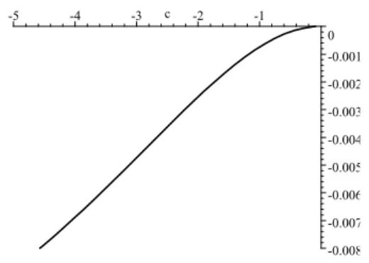
(a) The proof of Lemma 5 is similar to that of Lemma 3 and is omitted. (b) Figs. 3-4 plot the graphs ofdM1(c0, c0)in the casesg˜1t= (1, t)0andg˜2t=
¡
1, t, t2¢0,
respectively. The graphs reveal that dM1(c0, c0) < 0 for c0 < 0, and, therefore,
HnT >0forc0<0. -0.018 -0.016 -0.014 -0.012 -0.01 -0.008 -0.006 -0.004 -0.002 0 -5 -4 -3 c -2 -1
-0.008 -0.007 -0.006 -0.005 -0.004 -0.003 -0.002 -0.001 0 -5 -4 -3 c -2 -1
Fig. 4. Graph ofdM1(c0)when˜g2t=
¡
1, t, t2¢0.
(c) According to Moon and Phillips (2000), when c0 = 0, dM1(c0, c0) = 0 holds for
all polynomial trends g˜pt = (1, ..., tp)0. Also, for c0 = 0, direct calculations show
that dM2(c0, c0) = 0for g1t=t and dM2(c0, c0) = 0 forg2t=
¡
t, t2¢0. Therefore,
HnT →p0whenc0= 0,g1t=t,andg2t=¡t, t2¢0.
From Lemma 4 and the following remarks and by Assumption 6, it follows thatHnT
has a positive limit as(n, T → ∞)whenc0<0.Thus,HnT−1 =Op(1). Then, we can write
BnT2 ZnT(c) = MnT(c0)0W Mˆ nT(c0)− (BnTSnT)2 HnT +HnT µ BnT(c−c0)− BnTSnT HnT ¶2 +BnT(c−c0)BnTR1nT(c, c0) + (BnT(c−c0))2R2nT(c, c0). (22) Lemma 6 Under Assumptions 1-3 and Assumption 6, for every sequence γnT →0, we have as (n, T → ∞)following Assumption 5,
(a) sup c∈C:|c−c0|≤γnT |BnTR1nT(c, c0)|=op(1), and (b) sup c∈C:|c−c0|≤γnT |R2nT(c, c0)|=op(1).
Theorem 2 Suppose that Assumptions 1-3 and Assumption 6 hold. Then, as(n, T → ∞)
following Assumption 5,
BnT(ˆc−c0) =Op(1).
Lemma 6 establishes that the two remainder termsBnTR1nT(c, c0) andR2nT(c, c0)
converge in probability to zero uniformly in the shrinking neighborhood of the true param-eter. Also, Theorem 2 shows that the GMM estimator isBnT( =√n)−consistent. This
implies that in the shrinking neighborhood of the true parameter, the scaled objective functionB2
nTZnT(c)is uniformly approximated by the following quadratic function
BnT2 Zq,nT(c) = MnT(c0)0W Mˆ nT(c0)− (BnTSnT)2 HnT +HnT µ BnT(c−c0)− BnTSnT HnT ¶2 .
The heuristic ideas of the limit theory are as follows. LetBnT(ˆcq−c0) = arg min
c∈C B2
nTZq,nT(c).
Then, we may expect that a minimizer of B2
nTZnT(c) will be close to the minimizer of
B2
nTZq,nT(c),suggesting that the GMM estimatorBnT(ˆc−c0)will be close to BnT(ˆcq−c0) = BnTSnT HnT if ½ BnT(¯c−c0)≤ BnTSnT HnT ≤ − BnTc0 ¾ = BnT(¯c−c0) if ½ BnT(¯c−c0)> BnTSnT HnT ¾ = −BnTc0 if ½B nTSnT HnT >−BnTc0 ¾ . Notice that BnTSnT
HnT =Op(1) and recall that it is assumed that the true parameter
sat-isÞes¯c < c0<0. In this case, the probabilities of the events
n BnT(¯c−c0)> BnTHnTSnT o and n BnTSnT HnT >−BnTc0 o
will be very small and the scaled and centred estimatorBnT(ˆcq−c0)
will therefore be close with high probability to the random variable
ˆ
φnT = BnTSnT
HnT
.
In view of Lemmas 4 and 5 and Assumption 6,
BnTSnT ⇒S =d N¡0,σ8£dM(c0)0W J0Φ(c0)JW dM(c0)¤¢
and
HnT →pH=σ4dM(c0)0W dM(c0)>0
as(n, T → ∞)with nT →0.Thus, whenc0∈C0/{0}, ˆ
φnT ⇒φ=d H−1Slet=Z.
The proof of the following theorem conÞrms the heuristic argument above.
Theorem 3 Suppose that Assumptions 1-3 and Assumption 6 hold. Suppose that c0 ∈ C0/{0} and ˆc be the GMM estimator deÞned in (21). Then, as (n, T → ∞) following Assumption 5, √ n(ˆc−c0)⇒Z, where Z =d N Ã 0,dM(c0) 0W J0Φ(c0)JW dM(c0) £ dM(c0)0W dM(c0)¤ 2 ! . Remarks
(a) Whenc0∈C0/{0}andJ0Φ(c0)J is invertible, the optimal weight matrix is found
as
ˆ
Wopt = (J0Φ(ˆc)J)−1.
The limiting distribution of√n(ˆc−c0)is then
√ n(ˆc−c0)⇒Zopt=d N Ã 0, σ 4 £ dM(c0)0W dM(c0)¤ 2 ! . (23)
(b) Fig. 5 plots the graph of the minimum eigenvalue ofJ0Φ(c
0)J as a function ofc0.
As we see through the graph, J0Φ(c
0)J is positive deÞnite except for the case of c0= 0. Co 0.0 0.002 0.004 0.006 0.008 0.010 0.012 0.014 -10 -8 -6 -4 -2 0
Fig. 5. Graph of the Minimum Eigenvalue ofJ0Φ(c0)J wheng1t=t.
Co 0.003 0.004 0.005 0.006 0.007 0.008 0.009 -10 -8 -6 -4 -2 0
Fig. 6. Graph of the Minimum Eigenvalue ofJ0Φ(c0)J wheng2t=¡t, t2¢0.
4.3
Limiting Distribution of the GMM Estimator When
c0
= 0
An important special case of model 1 occurs whenc0= 0.The time series components of yitin(1) then have a unit root, and the deterministic trend is linear, so
zit = βi0t+yit (24)
where ρ0 = 1, i.e, c0 = 0. According to Remark (c) below Lemma 5, in this case, the
information from the moment conditions is zero becauseHnT →p 0.We cannot then use
a conventional quadratic approximation approach, as in the previous section, and need instead to employ a higher order approximation to extract the limit theory (c.f., Sargan, 1983).
This section develops asymptotics for the GMM estimator when the true localizing parameter is zero, so throughout this section we setc0= 0.The following lemmasÞnd the
limits of theÞrst and the second moment conditions and their higher order derivatives at
c= 0.
Lemma 7 Suppose that the panel data is generated by (24). Under Assumptions 2 and 3, the following hold as(n, T → ∞)following Assumption 5.
(a)√nM1nT(0)⇒N ³ 0,σ604´≡ q σ4 60Z,where Z≡N(0,1), (b)√ndM1nT(0) =N¡0,σ4 116300¢, (c)√nd2M1nT(0)⇒op(1), (d)d3M1nT(c)→pσ2d3M1(c,0) uniformly incwith d3M1(0) =−701,
wheredkM1nT(c) is thekth left derivative ofM1nT(c), and d3M1(c) is the third left derivative ofM1(c),the probability limit ofM1nT(c).
Lemma 8 Suppose that the assumptions in Lemma 7 hold. Then, when (n, T → ∞)
following Assumption 5, (a)√nM2nT(0) =op(1), (b)√ndM2nT(0)⇒N ³ 0,σ454´, (c)√nd2M 2nT(0) =op(1), (d)d3M 2nT(c)→pσ2d3M2(c)uniformly incwith d3M2(0) =−151, wheredkM
2nT(0) is thekthleft derivative of M2nT(c)at c= 0, andd3M2(0)is the third left derivative of d3M
2(c)atc= 0.
Remarks. Since the higher order derivatives of M2nT(0) are complicated and involve
extremely lengthy expressions, we omit the details of their derivation in the appendix. Instead, we give a sketch of the proof in the appendix and here provide some simulation evidence relating to the various parts of Lemmas 7 and 8. Using simulated data for zit
in (24) with εit ∼ iid N(0,1) and yi0 = 0, we estimate the means and the variances
of √ndkM
jnT(0), k= 0, ...,2; j = 1,2and the means ofd3MjnT(0), j = 1,2. Table 1
reports the results. The numbers in the table are consistent with the theoretical results in the lemmas. Noticeably, the variance estimates of √nM1nT(0), √ndM1nT(0), and
√
ndM2nT(0) are all small. This is because their theoretical limit variances are small
but not zero. In fact, a long calculation shows that the theoretical limit variances of
√nM
1nT(0), √ndM1nT(0),and √ndM2nT(0)are 601('0.01667), 630011 ('0.00175), and
1
45('0.0222), respectively whenεit∼iid N(0,1).
Table 19 9Notice that the second and the third derivatives ofM
√nM 1nT(0) √ndM1nT(0) √nd2M1nT(0) d3M1nT(c) Mean Variance −0.0019 0.018 −0.0003 0.0017 7.96×10⁻⁷ 0 −0.0169 N/A √nM 2nT(0) √ndM2nT(0) √nd2M2nT(0) d3M2nT(0) Mean Variance 9.4×10⁻⁵ 0.0012 −0.0001 0.022 −2.88×10⁻⁶ 4.85×10⁻⁶ −0.06 N/A
Using the left derivatives of the moment conditionMnT(c)atc= 0, we approximate
MnT(c)around the true parameterc0= 0with a third order polynomial as follows, MnT(c) =MnT(0) +c(dMnT(0)) + 1 2c 2¡d2M nT(0) ¢ +1 6c 3¡d3M nT(0) ¢ +c3r˜nT(c,0), where ˜ rnT(c,0) = (˜r1nT(c,0),r˜2nT(c,0))0, ˜ rknT(c,0) = d3MknT¡ck+¢−d3MknT(0), k= 1and2. Then, ZnT(c) = MnT(c)0W Mˆ nT(c) = 6 X k=0 ckAk,nT+NnT(c,0), where A0,nT = MnT(0)0W Mˆ nT(0), A1,nT = 2MnT(0)0W dMˆ nT(0), A2,nT = MnT(0)0W dˆ 2MnT(0) +dMnT(0)0W dMˆ nT(0), A3,nT = 1 3MnT(0) 0W dˆ 3M nT(0) +dMnT(0)0W dˆ 2MnT(0), A4,nT = 1 3dMnT(0) 0W dˆ 3M nT(0) + 1 4d 2M nT(0)0W dˆ 2MnT(0), A5,nT = 1 6d 2M nT(0)0W dˆ 3MnT(0), A6,nT = 1 36d 3M nT(0)0W dˆ 3MnT(0), and NnT(c,0) = 6 X k=3 ckNk,nT(c,0), Nk,nT(c,0) = αkd(k−3)MnT(0)0Wˆ˜rnT(c,0) fork= 3,4,5, N6,nT(c,0) = α6d3MnT(0)0Wˆr˜nT(c,0) + ˜rnT(c,0)0Wˆr˜nT(c,0), α3,α4 = 2, α5= 1, α6= 1 3,
whered0M
nT(0)denotesMnT(0).
In view of Lemmas 7 and 8, it is easy toÞnd that as(n, T → ∞)with n
T →κ<∞, n5/6A1,nT = op(1), (25) n2/3A2,nT = op(1), (26) n1/3A4,nT = op(1), (27) n1/6A5,nT = op(1), (28) and A6,nT → p σ4 36 µ W11 4900+ 2W12 1050 + W22 225 ¶ >0, (29) n1/2A3,nT ⇒ A3Z, (30) nA0,nT ⇒ A0Z2, (31) whereZ ≡N(0,1) andA3=−σ 2 3 ¡W11 70 + W12 15 ¢ qσ4 60 andA0=W11 σ4 60.
Also, using Lemmas 7 and 8 and following similar lines of proof to Lemma 6, we can show that sup c∈C:|c|≤γnT ¯ ¯¯n(6−k)/6Nk,nT(c,0) ¯ ¯¯=op(1), (32)
for any sequence γnT tending to zero as(n, T → ∞).Then, we have the following limit theory forˆcat the origin.
Theorem 4 Under the assumptions in Lemmas 7 or 8, and as (n, T → ∞) following Assumption 5,
n1/6(ˆc−c0) =Op(1), wherec0= 0.
So, when the true localizing parameter is c0 = 0, the GMM estimator ˆc is n1/6−
consistent,which is slower than the regular case of√nthat applies for c0 <0as shown
in Section 4. ToÞnd the limiting distribution ofˆc,we use an argument similar to that of the previous section. Consequently, we sketch the derivation and give the Þnal result in Theorem 5 below.
In view of (25)−(31)and (32), the standardized objective function nZnT(c)is
ap-proximated by Zq,nT(c) =nA0,nT + ³ n1/6c´ 3√ nA3,nT+ ³ n1/6c´ 6 A6,nT.
Notice that the probability limit ofA6,nT is positive, as shown in (29).Then, it is easy to
see that the approximate objective functionZq,nT(c)is minimized at
n1/6cˆq = − µ√ nA3,nT 2A6,nT ¶1/3 if ½ n1/6c¯≤ − √ nA3,nT 2A6,nT ≤ 0 ¾ = 0if ½ − √ nA3,nT 2A6,nT >0 ¾ = −³n1/6(−¯c)´1/3 if ½ n1/6¯c >− √ nA3,nT 2A6,nT ¾ .
Using arguments similar to those in the proof of Theorem 3, we can prove that the standardized GMM estimatorn1/6ˆcis approximated byn1/6ˆc
q,the minimizer ofZq,nT(c),
that is,
n1/6ˆc=n1/6ˆcq+op(1),
and the estimator n1/6cˆqis approximated by
ˆ φnT =− µ√n A3,nT 2A6,nT ¶1/3 1 ½ − √n A3,nT 2A6,nT ≤ 0 ¾ ,
where 1{A} is the indicator of A. In view of (30) and (29), as (n, T → ∞) following Assumption 5,it follows by the continuous mapping theorem that
ˆ φnT ⇒Z01/31{Z0≤0}, where Z0 = V0Z, (33) V0 = ¯ ¯ ¯ ¯ ¯¯ q 1 15 ¡W11 70 + W12 15 ¢ 1 3 ¡W11 4900+ 2W12 1050 + W22 225 ¢ ¯ ¯ ¯ ¯ ¯¯, (34)
and Wij are the (i, j)th element of the weight matrix W. Thus, we have the following
theorem.
Theorem 5 Under the assumptions in Lemmas 7 and 8, as (n, T → ∞) following As-sumption 5,
n1/6ˆc⇒Z01/31{Z0≤0}, where Z0 is deÞned in(33).
Remarks
(a) Theorem 4 shows that when the true parameter c0= 0, i.e.,in the case of a panel
unit root, the GMM estimator is n1/6-consistent and that its limit distribution is
nonstandard, involving the cube root of a truncated normal. The truncation in the limiting distribution arises because the true parameter is on the boundary of the parameter set.
(b) The reason for the slower convergence rate in the panel unit root case is thatÞrst order information in the moment condition (from the Þrst derivative of the mo-ment condition) is aymptotically zero at the true parameter. In order to obtain nonneglible information from the moment condition, we need to pass to third order derivatives of the moment condition. Taking the higher order approximation slows down the convergence rate because the rate at which information in the moment condition is passed to the estimator is slowed down at the origin because of the zero lower derivatives.
(c) In view of Lemmas 7(a) and 8(a), weÞnd that√nM2nT(0) =op(1),while√nM1nT(0)
converges in distribution to a normal random variable with positive variance. Be-cause of the convergence rate difference between√nM2nT(0)and√nM1nT(0),we
setting W11 = W12 = 0, i.e. not considering the Þrst moment condition, causes
the variance of the limit variateZ0 in(33)to vanish, from which one might expect
that the GMM estimator from the second moment condition alone would have a faster convergence rate thann1/6. The reason for using theÞrst moment condition
is to identify the true parameterc0whenc0<0.As we discuss in Appendix D, the
second moment condition cannot identify the true parameterc0unlessc0= 0.
4.4
On Testing for a Unit Root
This section brießy considers how the asymptotic results for the localizing coefficient given in the previous section may be used to test for a unit root in the panel. Suppose the null hypothesis is H0 : c0 = 0 and the alternative hypothesis is H1 : c0 <0. We discuss two
types of panel unit root tests, one involving at−test and the other an LM test.
First, Theorem 5 shows that to testH0we can use a suitably constructedt−statistic.
SpeciÞcally, letVˆ0 be a consistent estimator ofV0and deÞne tgmm= √ nˆc3 ˆ V0 .
Then, sinceVˆ0→pV0 and from Theorem 5 with(n, T → ∞)as in Assumption 5, we get tgmm⇒Z1{Z ≤0},
whereZ ≡N(0,1).Under the alternative hypothesis c=cA<0,we have
tgmm = √n¡ˆc3−c3 A ¢ ˆ V0 + √nc3 A ˆ V0 = Op(1) + √nc3 A ˆ V0
by Theorem 3 and the delta method. So, under the alternative hypothesis,tgmm→ −∞
and the test is consistent.
Another type of test is to use the asymptotic properties of the moment conditions in Lemmas 7 and 8 in conjunction with the restricted parameter estimator, which is zero in this case. For example, in Lemma 7 we observe that √ndM1nT(0) = N
¡
0,σ4 11 6300
¢
.
Thus, a simple test can be based on
LMgmm= Ãr 6300 11 √ ndM1nT(0) ˆ σ2 !2 .
Then, as(n, T → ∞)as in Assumption 5, we have
LMgmm⇒χ2(1).
Under the alternativec=cA<0,it is easy to show that(√ndM2nT(0))
2
=nO(1)2→ ∞,
whiled3M
2nT(0)→p−σ2 115 <0.Thus, under the alternative hypothesis,LMgmm→ ∞.
The same principle can be applied to the second moment conditionM2nT(0).
5
Conclusion
Part of the richness of panel data is that it can provide information about features of a model on which time series and cross section data are uninformative when they are used on
their own. In the context of nonstationary panels with near unit roots, an interesting new example of this ‘added information’ feature of panel data is that consistent estimation of the common local to unity coefficient becomes possible. This means that panel data help to sharpen our capacity to learn from data about the precise form of nonstationarity where time series data alone are insufficient to do so. However, as the authors have shown in earlier work, the presence of individual deterministic trends in a panel model introduces a serious complication in this nice result on the consistent estimation of a root local to unity. The complication is that individual trends produce an incidental parameter problem as
n → ∞ that does not disappear as T → ∞. The outcome is that common procedures like pooled least squares and maximum likelihood are inconsistent. Thus, the presence of deterministic trends continues to confabulate inference about stochastic trends even in the panel data case.
One option is to adjust procedures like maximum likelihood to deal with the bias. The present paper shows how to make these adjustments. The theory is cast in the context of moment formulae that lead naturally to GMM based estimation. The paper has two importantÞndings.
The Þrst is that bias correction in the moment formulae arising from GLS estima-tion of the trend coefficients corresponds to taking the projected score (under Gaussian assumptions) on the Bhattacharya basis. This correspondence relates the approach we take here to recent work on projected score methods by Waterman and Lindsay (1998) that deals with models that have inÞnite numbers of nuisance parameters like the original incidental parameters problem.
The second is that our limit theory validates GMM-based inference about the localizing coefficient in near unit root panels. A notable new result is that the GMM estimator has a convergence rate slower than√nwhen the true localizing parameter is zero (i.e., when there is a panel unit root) and the deterministic trends in the panel are linear. The asymptotic theory in this case provides a new example of limit theory on the boundary of a parameter space. The results point to the continued difficulty of distinguishing unit roots from local alternatives when there are deterministic trends in the data even when time series data is coupled with an inÞnity of additional data from a cross section.
6
Appendix
6.1
Proof of the Equivalence Lemma
Before we start the proof of Lemma 1, we give some useful background results.
Lemma 9 LetKmdenote the(m×m)commutation matrix,Dmdenote them2×12m(m+ 1) duplication matrix, and set D+
m = (D0mDm)−1Dm0 . Also, assume that x andy are m−
vectors andAis an (m×m)invertible matrix. Then the following hold. (a)xy0⊗yx0=Km(yy0⊗xx0). (b)(Im+Km) ((x⊗y) + (y⊗x)) = 2 (x⊗y) + 2 (y⊗x). (c)Dp+Dp=I1 2p(1+p). (d)DpD+p = 12(Ip+Kp). (e)¡D+ p (A⊗A)Dp¢− 1 =D+ p ¡ A−1⊗A−1¢D p. Proof
Parts (c), (d), and (e) are standard results (e.g., Magnus and Neudecker, 1988, pp. 49-50). Part (a) holds because
xy0⊗yx0 = (x⊗y) (y0⊗x0) =vec(yx0) (vec(xy0))0
= (Kmvec(xy0)) (vec(xy0))0 =Km(y⊗x) (y⊗x)0
= Km(yy0⊗xx0).
Part (b) holds because
(Im+Km) ((x⊗y) + (y⊗x))
= (x⊗y) + (y⊗x) +Kmvec(yx0) +Kmvec(xy0)
= (x⊗y) + (y⊗x) +vec(xy0) +vec(yx0) = 2 (x⊗y) + 2 (y⊗x).¥
Proof of Lemma 1
In this proof we omit the subscriptpthat denotes the order of the polynomial trends for notational simplicity. To complete the proof, it is enough to show that λT(c) in
m2,iT(c)is equivalent toξ02D+p PT t=1(∆cgt⊗∆cgt)inU2i ³ c,βˆi(c)´.First, we deÞne ˜ A1T = 1 T T X t=2 1 T t−1 X s=1 D+p h∆[cgt⊗∆[cgs+∆[cgs⊗∆[cgt i ·³ 1 + c T ´T¸t−Ts−1 , ˜ A2T = 1 T T X t=1 1 T T X s=1 D+p n³∆[cgt∆[cgt 0 ⊗∆[cgs∆[cgs 0´ +³∆[cgt∆[cgs 0 ⊗∆[cgs∆[cgt 0´o ¡ Dp+¢0, ˜ A3T = D+p 1 T T X t=1 ³ [ ∆cgt⊗∆[cgt ´ .
Then, by deÞnition, we write
ξ02D+p T
X
t=1
(∆cgt⊗∆cgt) = ˜A10TA˜−2T1A˜3T.
Notice by Lemma 9(a), (d), and (c) that
˜ A2T = Dp+(Ip+Kp) 1 T T X t=1 1 T T X s=1 ³ [ ∆cgt∆[cgt 0 ⊗∆[cgs∆[cgs 0´ ¡ D+p¢0 = 2D+pDpD+p "à 1 T T X t=1 [ ∆cgt∆[cgt 0! ⊗ à 1 T T X s=1 [ ∆cgs∆[cgs 0!#¡ D+p¢0 = 2D+p "à 1 T T X t=1 [ ∆cgt∆[cgt 0! ⊗ à 1 T T X s=1 [ ∆cgs∆[cgs 0!#¡ D+p¢0 = 2 " D+p à 1 T T X t=1 [ ∆cgt∆[cgt 0! ⊗ à 1 T T X s=1 [ ∆cgs∆[cgs 0! Dp # ¡ Dp0Dp ¢−1 .
By Lemma 9(e), ˜ A−2T1 = 1 2 ¡ D0pDp ¢ D+p à 1 T T X t=1 [ ∆cgt∆[cgt 0!− 1 ⊗ à 1 T T X s=1 [ ∆cgs∆[cgs 0!− 1 Dp = 1 2D 0 p à 1 T T X t=1 [ ∆cgt∆[cgt 0!− 1 ⊗ à 1 T T X s=1 [ ∆cgs∆[cgs 0!− 1 Dp.
Again, from Lemma 9(d) and (b), we have
˜ A01TA˜−2T1A˜3T = 1 T T X t=2 1 T t−1 X s=1 h [ ∆cgt⊗∆[cgs+∆[cgs⊗∆[cgt i0·³ 1 + c T ´T¸t−sT−1¡ D+p ¢0 ×12D0p à 1 T T X t=1 [ ∆cgt∆[cgt !−1 ⊗ à 1 T T X s=1 [ ∆cgs∆[cgs 0!− 1 Dp ×D+p 1 T T X t=1 ³ [ ∆cgt⊗∆[cgt ´ = 1 8 " 1 T T X t=2 1 T t−1 X s=1 h [ ∆cgt⊗∆[cgs+∆[cgs⊗∆[cgt i0·³ 1 + c T ´T¸t−Ts−1# (Ip+Kp)0 × Ã 1 T T X t=1 [ ∆cgt∆[cgt !−1 ⊗ à 1 T T X s=1 [ ∆cgs∆[cgs 0!− 1 ×(Ip+Kp) " 1 T T X t=1 ³ [ ∆cgt⊗∆[cgt ´# = 1 2 " 1 T T X t=2 1 T t−1 X s=1 h [ ∆cgt⊗∆[cgs+∆[cgs⊗∆[cgt i0·³ 1 + c T ´T¸t−Ts−1# × Ã 1 T T X t=1 [ ∆cgt∆[cgt !−1 ⊗ à 1 T T X s=1 [ ∆cgs∆[cgs 0!− 1 × " 1 T T X t=1 ³ [ ∆cgt⊗∆[cgt ´# . (35) Expanding(35)yields 1 T T X t=2 1 T t−1 X s=1 1 T T X p=1 ·³ 1 + c T ´T¸t−Ts−1h [ ∆cgs 0 A−pT1∆[cgp i h [ ∆cgp 0 A−pT1∆[cgt i = 1 T T X t=2 1 T t−1 X s=1 ·³ 1 + c T ´T¸t−Ts−1 [ ∆cgs 0 A−pT1∆[cgt = λpT(c).¥
6.2
Appendix A: Useful Results for Joint Asymptotics
This section consists of two subsections. TheÞrst subsection introduces some useful results for joint asymptotic theories. Many of these are modiÞed versions of results developed in Phillips and Moon (1999) so we report them only brießy here. The second subsection introduces some useful results which will be used repeatedly in the fo