2013/36
■
Spatial issues on a hedonic estimation
of rents in Brussels
Alain Pholo Bala, Dominique Peeters
and Isabelle Thomas
Center for Operations Research
and Econometrics
Voie du Roman Pays, 34
B-1348 Louvain-la-Neuve
Belgium
http://www.uclouvain.be/core
D I S C U S S I O N P A P E R
CORE DISCUSSION PAPER 2013/36
Spatial issues on a hedonic estimation of rents in Brussels
Alain PHOLO BALA 1, Dominique PEETERS2
and Isabelle THOMAS 3
July 2013
Abstract
Using Belgian microdata, we assess the impact, on a hedonic regression, of the distortions arising from the choice of either a specific zoning system or the delineation of the study area. We also evaluate the biases that arise when spatial effects are not accounted for. Given that the dependent variable is interval-coded, controlling for spatial dependence in this context is challenging. We address this problem with two alternative strategies. Firstly, we use the Gibbs Sampling algorithm to estimate spatial econometric models which extends the interval regression model. A major drawback of this approach is that the implied estimation is proned to the endogeneity biases inherent to our hedonic regression model. To circumvent the endogeneity issues triggered by the first estimation strategy, we also use a two-stage estimation procedure with locational fixed effects. In all specifications, results are sensitive to the Modifiable Areal Unit Problem (MAUP) and to the choice of the delineation of the study area. Moreover, they confirm the existence of substantive spatial dependence. Conversely to the previous results with a negative elasticity for the percentage of the area covered by agriculture and a positive elasticity for the potential accessibility to jobs, the second approach implies opposite effects for those two variables. This indicates that dwellings close to agricultural areas and with a lower accessibility to the main employment centers are highly demanded and that endogeneity biases are not negligible.
Keywords: MAUP, interval regression, spatial dependence, spatial heterogeneity, Brussels.
JEL Classification: C21, C24, C25, C34, Q53, R21
1 Department of Economics and Econometrics, University of Johannesburg, South Africa. E-mail: [email protected] 2Université catholique de Louvain, CORE, B-1348 Louvain-la-Neuve, Belgium.
E-mail: [email protected]. This author is also member of ECORE, the association between CORE and ECARES.
3 Université catholique de Louvain, CORE, B-1348 Louvain-la-Neuve, Belgium.
E-mail: [email protected]. This author is also member of ECORE, the association between CORE and ECARES.
1
Introduction
The increasing concerns about sustainable development and the growth of urban areas have facilitated a renewed enthusiasm for the use of quantitative models in the field of transportation and spatial planning.
Some spatial issues may arise from the implementation of those quantitative models. One of them is that their implementation requires a massive amount of geographic data collected from various sources, and often at different spatial scales. Another issue is that the definition of agglomerations or, more broadly, the delineation of the study area may differ in the different case studies. All those problems are likely to influence and bias spatial econometric analyses. Moreover, spatial autocorrelation is also likely to have significant impacts on statistical findings. In this paper, we check the magnitude of those “spatial” biases and we propose some sug-gestions to control or at least limit them. To do so we will base our econometric investigation on the first–stage hedonic regression model, which is well represented in the OPUS/UrbanSim platform as the Real Estate Price Model.
In a conceptual point of view, the problem of spatial autocorrelation and the issues of the choice of spatial scales and of the study area boils down to spatial dependence and spatial heterogeneity problems. Spatial dependence is one of the main methodological problems that has to be tackled in first–stage hedonic regression. In general terms, it may be “considered to be the existence of a functional relationship between what happens at one point in space and what happens elsewhere” (Anselin, 1988, p.11).
Two broad causes may lead to spatial dependence: the nuisance and the substantive spatial dependence (Magrini, 2004). The nuisance spatial dependence refers to the by-product of mea-surement errors for observations in contiguous spatial units. In several cases data are collected only at aggregate scale. As it implies a poor correspondance between the spatial scope of the phenomenon under scrutiny and the delineation of the spatial units of observations, it may entail measurement errors. Those errors will tend to spill over across the frontiers of spatial entities as one may expect that errors for observations in one spatial unit are likely to be correlated with errors of neighboring geographical entities (Anselin, 1988).
Such measurement errors may be caused by problems of spatial aggregation or by arbitrary delineation of spatial units of observations. The aggregation of spatial data is not benign regard-ing statistical inference. The question of the sensitivity of statistical results to the choice of a particular zoning system is well known as the Modifiable Areal Unit Problem (MAUP).
Several contributions have assessed the impact of the MAUP on multivariate statistics (Gehlke and Biehl, 1934; Fotheringham and Wong, 1991; Amrhein, 1995; Briant et al., 2010). Gehlke
and Biehl (1934) outline the tendency for the correlation coefficient to increase as the size of spatial units increases. In a recent contribution, Briant et al. (2010) analyze the impact of size distortions on the behavior of simple regression coefficients. The context of our study is somewhat different since, as the dependent variable and several covariates are individual dwelling attributes, aggregation biases apply only to a subset of regressors.
Nuisance spatial dependence may also arise because of the arbitrary delineation of basic spatial units (BSU). In a literature review on regional convergence, Magrini (2004) makes an interesting survey of the question. He asserts that the use of administratively defined regions raises two fundamental problems: on the one hand, since output is measured at workplaces while population at residences, the measured levels of per capita income will be highly misleading. On the other hand, processes of decentralization or recentralization of residences relative to workplaces is likely to affect per capita income growth rates for administratively defined regions. A related but less investigated issue is the one arising from the choice of the delineation of the study area. This issue points more to spatial heterogeneity, i.e. the lack of uniformity of the effects of space. Any structural instability of a given relationship across space would entail different econometric results for distinct study areas. More intuitively, different limits of agglom-eration entail distinct geographic structures; and therefore unequal features in terms of degree of urbanization and accessibility. Our contribution focuses on Brussels. For this specific city several delineations may be considered: administrative delineations, morphological delineations (Don-nay and Lambinon, 1997; Tannier et al., 2011; Van Hecke et al., 2009), functional delineations (Cheshire, 2010; Van Hecke et al., 2009; Vandermotten et al., 1999), etc. While each way of defining Brussels may be consistent according to a given standpoint, considering administrative definitions can be harmful since administrative borders do not capture the essence of economic phenomena and transportation issues that often spill over boundaries. In this paper, we analyze nuisance spatial dependance and spatial heterogeneity by investigating the impacts of choices of the aggregation scale and of the delineation of the study area.
The substantive spatial dependence is more fundamental and is due to varieties of interdepen-dencies across space. Location and distance do matter and formal frameworks proposed by spatial interaction theories, diffusion processes and spatial hierarchies structure the dependence between phenomena at different locations in space (Anselin, 1988). It has been amply demonstrated that the neglect of spatial considerations in econometric models not only affects the magnitudes of the estimates and their significance, but may also lead to serious errors in the interpretation of standard regression diagnostics such as tests for heteroskedasticity (Kim et al., 2003).
In this paper, we also assess substantive spatial dependence by considering three components of the spatial econometrics toolbox: the Spatial AutoRegressive Model (SAR), the Spatial Durbin
Model (SDM) and the General Spatial Model (SAC). Several contributions investigate the spatial dependence issue in cross–sectional hedonic price analyses through the estimation of Spatial Models (Gawande and Jenkins–Smith, 2001; Kim et al., 2003; Brasington and Hite, 2005; L¨ochl and Axhausen, 2010).
In most of these contributions, the dependent variable (house price or dwelling rent) is con-tinuous. In this paper, we have to face an extra problem: the information about the dependent variable (here: dwelling rent) is collected through a categorical variable. Each modality of this discrete variable refers to a unique interval of dwelling rents. Therefore, we have to resort to techniques designed to estimate spatially dependent discrete choice models.
There are two ways to handle this issue. The first approach consists on using a Gibbs Sampling algorithm to design “Spatial Interval Regression” models. The second approach implies the use of a two-step procedure where we perform in the first step an interval regression on structural characteristics and fixed/locational effects. Then, in the second step we retrieve fixed/locational effects to obtain averages of log of rents within the basic spatial units and we regress them on a set of observed location characteristics. This last approach has the advantage of avoiding endogeneity bias caused by locational characteristics. Indeed, one may suspect reverse causality between dwelling rents and location characteristics like average income or accessibility.
This paper is organized as follows. The next section is devoted to a detailed presentation of the estimation strategy. The third section describes the study area and section 4 presents the data used for estimation. Section 5 presents the results of estimations and section 6 concludes the paper.
2
Estimation strategy
We estimate the hedonic model by means of interval regression and we analyze spatial effects. In this section we present the methodological aspects of our two estimation approaches.
2.1
Benchmark model: interval regression
In some databases the information on rent prices is collected through a categorical variable (cfr. 4.1). Therefore, they do not give the actual value of the rent yi∗; they just provide the value yi
of a categorical variable from which we can infer the interval where y∗i lies:
yi =j if αj−1 < y∗i ≤αj
where j ∈ {1, ..., J} and α = (α0, α1,· · · , αJ) is a given vector of boundaries with α0 ≤ α1 ≤
To estimate this model, without taking spatial effects into account, we rely on an “interval regression”. This model is close to the ordered probit model from a computational perspective, but it is conceptually different, since it may be interpreted as an extension of censored regression.1
In such a framework, y∗ = (y∗1, y2∗,· · · , y∗N)0 is a variable that has a quantitative meaning and not just a latent variable with only an ordinal signification, as in the ordered probit model (Wooldridge, 2002). This computational procedure presents some important differences with the ordered probit model: in the latter the vector α is an ordered set of unknown cut points. Therefore, there is an identification issue in the ordered probit model andσ2 =V ar(y∗|X) (with
X the matrix of regressors) is normalized to one so that the model can estimateβ, the vector of regressors, andα. In the interval regression modelαis rather a set of known interval boundaries, thus, β and σ2 may be jointly estimated.
As in Geoghegan et al. (1997), we opt for double-log estimation. This functional form has the clear advantage of simplifying the interpretation of the estimated coefficients of continuous variables. Therefore, in this model we are interested in estimating E(ln (y∗i)|x) =xi0β where xi
denotes a vector of dummies and of logarithmic transformations of continuous variables.
2.2
Spatial Interval Regression Models
2.2.1 DescriptionA first approach to control for spatial dependence is to extend the basic Interval Regression model by the following specification:
˜
y = ρW1y˜+Xβ+u
u = λW2u+ (1)
∼ N 0, σ2IN
where ˜y = ln (y∗), N is the number of observations, X is a N ×k matrix of regressors, ρ is the spatial dependence parameter. Whenever W1 6= 0 and W2 6= 0, we assume that W1 =W2 = W
which are N ×N standardized spatial weight matrices.
W tells us whether any pair of observations are neighbors. For example, if dwelling i and dwelling j are neighbors then,wij = 1 and zero otherwise. Whether or not any pair of dwellings
are neighbors is based on whether or not they are located in the same geographical entity or
1Extreme values of the categories on either end of the range are either left–censored or right–censored. The
other categories are interval censored, that is, each interval is both left and right censored. Source: SAS Data Analysis Examples, Interval Regression. UCLA: Academic Technology Services, Statistical Consulting Group from http://www.ats.ucla.edu/stat/sas/dae/intreg.htm(last access June 03, 2013).
in contiguous spatial units. We follow Kim et al. (2003) by considering two spatial units as contiguous when they share a common border.
We assume that there areSspatial entities. Any spatial entitylis populated byNlindividuals,
with PS
l=1Nl=N. Therefore, ify
∗
sl denotes the Nl×1 vector of rents paid by the Nl households living in the lth spatial entity, the N×1 vector of rents paid by all the households of the sample is y∗ = y∗s10,· · ·, y∗s
l
0
,· · · , ys∗S00.
While much has been written on the techniques for dealing with spatial dependence in con-tinuous econometric models, the study of spatial dependence in discrete choice models has re-ceived less attention in the literature. This is clearly due to the added complexity that spatial dependence introduces into discrete choice models and the subsequent need for more complex estimators.
Several techniques are used to estimate this spatially dependent discrete choice model in a purely cross-sectional setting. A comprehensive review of those techniques may be found in Flemming (2004). In this paper we opt for the Gibbs Sampling approach since it outperforms the most relevant alternative methods: the Recursive Importance Sampling (RIS) simulator and the Expectation Maximization (EM) algorithm. Indeed, while providing results that are similar to those of the RIS simulator, it is computationally and conceptually simpler (Bolduc et al., 1997). Moreover, the Gibbs Sampler method overcomes the problem encountered in the estimation of standard errors by the EM algorithm because the standard errors of the estimates are derived directly from the posterior parameter distributions.
Specification (1) describes the SAC model. This model contains spatial dependence in both the dependent variable and the disturbances (LeSage and Pace, 2009). IfW2 = 0, then model (1)
simplifies to the SAR model. The SAR model implicitly assumes thatW1y˜, the spatially weighted
average of housing prices in a neighborhood, affects the price of each dwelling (indirect effects) in addition to the standard explanatory variables of housing and neighborhood characteristics (direct effects). It is particularly appropriate when there is structural spatial interaction in the market and the modeler is interested in measuring the strength of that relationship. As the assumption of structural spatial interaction is peculiarly relevant in the hedonic regression, it is our favorite modelling strategy. It is also relevant when the modeler is interested in measuring the “ “true” effect of the explanatory variables, after the spatial autocorrelation has been removed” (Kim et al., 2003, p. 29).
Assuming thatW2 = 0 allows to develop an extension of the SAR model, the Spatial Durbin
model (SDM) which controls for spatial dependence in the dependent variable and the explana-tory variables. The formal expression of the SDM model is shown in (2):
˜
y = ρW y˜+Xβ+W Xθ+ (2)
∼ N 0, σ2IN
where X denotes the matrix of regressors with the intercept excluded. The W X term al-lows the physical attributes of neighboring dwellings to impact the rent of each dwelling. It further captures how the price of houses in one BSU depends on the environment quality and the neighborhood characteristics of contiguous BSUs (Brasington and Hite, 2005).
The SAC model is the additive combination of the Spatial Error Model (SEM) and the SAR Model. Whenever W1 = 0, the SAC model collapses to the SEM Model defined by the following
specification:
˜
y=Xβ+u u=λW u+ ∼ N 0, σ2IN
. (3)
2.2.2 Estimation of SAR or SDM Interval Regression Models
SAR and SDM models can be written by the same expression
˜
y = ρW y˜+Zδ+ (4)
∼ N 0, σ2IN
where Z =X for the SAR model and Z = [X W X] for the SDM model.
This implies that the likelihood function for SAR and SDM models can be expressed in the same way L y, W˜ |ρ, δ, σ2 = 1 (2πσ2)N2 |IN −ρW|exp − 1 2σ2( 0 ) (5) where = (IN −ρW) ˜y−Zδ.
Using diffuse priors for (δ, σ2, ρ) results in the following expression of the joint posterior
density, we have: p δ, σ2, ρ|y, Z, W˜ ∝ |IN −ρW| σ2 −(N/2+1) exp − 1 2σ2 ( 0 ) (6) Estimates of this distribution should be sampled through a Gibbs sampler with the following 4 steps:
1. Drawing δ frompδ|σ2 (0), ρ(0),y˜(0) δ|σ(0)2 , ρ(0),y˜(0) ∼ N ˜ δ, σ(0)2 (Z0Z)−1; (7) ˜ δ = (Z0Z)−1(Z0Ay˜) ; (8) A = IN −ρW. (9) 2. Drawing σ2 from p σ2|δ(1), ρ(0),y˜(0) σ2|δ(1), ρ(0),y˜(0) ∼ σ2 −(N/2+1) exp − 1 2σ2 ( 0) . (10) 3. Sample pρ|δ(1), σ2(1),y˜(0)
by inversion approach (LeSage and Pace, 2009), where
p ρ|δ, σ2,y˜∝ |A|exp − 1 2σ2 ( 0 ) . (11)
4. Drawing ˜y from theN (µ,Ω) distribution ˜ y|δ(1), σ2(1), ρ(1) ∼ T M V N(µ,Ω) ; (12) µ = (IN −ρW) −1 Zδ; (13) Ω = σ2(IN −ρW) 0 (IN −ρW) −1 ; (14)
where TMVN denotes a multivariate truncated normal distribution.
The conditional distribution of ρ does not take a known form as in the case of the conditionals for the parameters δ and σ2. Therefore, sampling for the parameter ρ must proceed using an
alternative approach, such as numerical integration or Metropolis-Hastings.
2.2.3 Estimation of a General Spatial Interval Regression Model
Assuming that W1 =W2 =W 6= 0, we have to estimate the more general SAC model described
in (1). With Z =X, the associated likelihood concentrated for the parametersδ andσ2 take the following form (LeSage and Pace, 2009):
p y˜|δ, σ2, ρ, λ ∝ |A| |B|exp − 1 2σ2 (BAy−BZδ) 0 (BAy−BZδ) (15) with A = IN −ρW, and B = IN −λW
Following LeSage and Pace (2009), we draw the estimates of this distribution through the following 5 steps Gibbs sampler:
1. Drawing δ frompδ|σ2 (0), ρ(0), λ(0),y˜(0) δ|σ2(0), ρ(0), λ(0),y˜(0) ∼ N ˜ δ, σ(0)2 (Z0B0BZ)−1; (16) ˜ δ = (Z0B0BZ)−1(Z0B0Ay˜). (17) 2. Drawing σ2 from p σ2|δ (1), ρ(0), λ(0),y˜(0) σ2|δ(1), ρ(0), λ(0),y˜(0) ∼ σ2 −(N/2+1) exp − 1 2σ2 ( 0 ) , (18) with = B(Ay˜−Zδ) (19) 3. Sample pρ|δ(1), σ2(1), λ(0),y˜(0)
by inversion approach (LeSage and Pace, 2009), where
p ρ|δ, σ2, λ,y˜ ∝ |A|B λ(0) exp − 1 2σ2 ˜ B(Ay˜−Zδ) 0 ˜ B(Ay˜−Zδ) . (20) 4. Sample pλ|δ(1), σ(1)2 , ρ(0),y˜(0)
by inversion approach (LeSage and Pace, 2009), where
p λ|δ, σ2, ρ,y˜∝ A ρ(0) |B|exp − 1 2σ2 B ˜ Ay˜−Zδ 0 B ˜ Ay˜−Zδ . (21)
5. Drawing ˜y from theN (µ,Ω) distribution ˜ y|δ(1), σ(1)2 , ρ(1), λ(1) ∼ T M V N(µ,Ω) ; (22) µ = (IN −ρW) −1 Zδ; (23) Ω = σ2[A0B0BA]−1. (24)
When sampling for the parameter ρ (λ), we rely on the current value for λ (ρ) in |B| (|A|) which we denoteB λ(0) A ρ(0) , andB λ(0) = ˜BA ρ(0)
= ˜A. Therefore, we can still perform our univariate numerical integration scheme to find a normalizing constant and produce a CDF from which we can draw by inversion.
2.3
Two-step estimation with locational fixed effects
Spatial econometrics models described in section 2.2 are designed for purely cross-sectional set-tings. However, since our database has several observations (dwellings) for each basic spatial unit, it has the structure of a panel. Therefore, we may control for location heterogeneity by using an interval regression model with location/fixed effects.
Such an estimation strategy has an additional advantage as it allows to avoid the endogeneity bias caused by locational characteristics. One may suspect reverse causality between dwelling rents and observed location characteristics like average income or accessibility. While we may expect dwelling rents to be high as a resultant of high average income in the area, we may as well consider areas with high dwelling rents as a sign of attractiveness for high income households because they are expected to host better schools or because they host socio-economic peers.
Since reverse causality is more likely to concern location invariant attributes, we may address this endogeneity problem by retrieving locational fixed effects. Hence, we use an alternative approach to capture spatial dependence based on a two-stage procedure (Ahlfeldt, 2011). In the first stage we obtain estimated values of dwelling rents by carrying out an interval regression on a set of dwelling structural attributes as well as a set of locational-fixed effects that capture location heterogeneity ˜ yi = zi0α+µl+εi or equivalently (25) ˜ y = Zsα+Zµµ+ε (26) with ε ∼ N(0, σ2 εIS), Zs = z10 z20 .. . zN0 and µ = (µ1, µ2, . . . , µS) 0 where Zs is a N ×ks matrix of
dwellings structural characteristics2,α is the corresponding vector of coefficients, µis a vector of unobserved location fixed effects, and Zµ is a N ×S matrix of spatial entities dummies. After
this first step, we retrieve the fixed effects and obtain an estimate of the average log of dwelling rent within former townships LREN T, adjusted for dwelling characteristics.
Then in a second stage, we regress LREN T on location characteristics
LREN Tj =LOCj0γ+ηj (27)
where LREN T is the average log of dwelling rents estimated from specification (26),LOC is a row-vector of location controls,γ is the corresponding column vector of coefficient estimates and
η is a random error term.
This two-step estimation strategy ensures that there is no endogeneity bias due to the corre-lation between unobserved location characteristics and observed neighborhood and environment quality attributes.
2withk
We may account for spatial dependence in this second stage by extending (27) into a general spatial model
LREN T = δM1LREN T +LOCγ+η
η = φM2η+ξ (28)
ξ ∼ N 0, σ2ξIS
where δ is a spatial dependence parameter, M1 and M2 are S×S standardized spatial weight
matrices which tell whether two spatial entities are neighbors or not. As before, (28) simplifies to a SAR model if M2 = 0. Moreover, in estimating (28) we will assume that M1 =M2 =M.
3
Delineation of the study area and basic spatial unit
3.1
Delineation of the study area
We restrict the focus of our analysis to the private renting market of Brussels. Here comes the first spatial issue as there is no univocal definition of Brussels. Several delineations of the capital of Belgium have been proposed based on different criteria, namely, administrative, morphological (Donnay and Lambinon, 1997; Tannier et al., 2011; Van Hecke et al., 2009) and functional (Cheshire, 2010; Van Heckeet al., 2009; Vandermottenet al., 1999; Blondelet al., 20103, Thomas
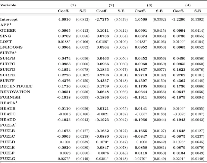
et al., 2012). Table 2 and Figure 1 in Appendix B present macrozones that are consistent with eight delineations of Brussels. One of those delineations, the Brussels Capital Region, corresponds to a purely administrative definition of Brussels. Another delineation, Brussels (operational) agglomeration corresponds to a morphological definition of Brussels. It is one of the macrozones defined by the Van Hecke et al. (2009) nomenclature of Belgian urban regions.
The other delineations represent merely functional definitions of Brussels. They are macro-zones that, because of the strong socio-economic ties of their peripheral rings with the Brussels urban center, may serve to define the Brussels urban functional region. From the Van Hecke
et al. (2009) nomenclature, we may consider the Brussels urban region on one hand and the
3The methodology used by Blondel et al. (2010) to define a functional agglomeration is quite innovative.
They use a mathematical method, based on origin-destination matrices, which allows networks to be divided into coherent groups in a natural and automatic manner (modularity criteria). This generates a mathematically optimal partition of space. Another innovative method is the one used by Rozenfeldet al. (2011). Rather than using informative but somewhat arbitrary legal or administrative definitions, they build on the City Clustering Algorithm (CCA) to construct cities based on geographical features of high-quality micro data.
Brussels residential urban complex on the other hand. We may also consider Brussels “extended residential commuting complex” which is the union of the Brussels and Leuven residential com-muting complexes. Stratec, an independent consultancy company, has proposed other definitions: “Stratec RER Area” and “Stratec Extended RER Area” on the basis of commuting ties through the railway network transportation system.4
The 2001 Belgian census includes the information from 177,721 dwellings pertaining to the Brussels Capital Region and 330,147 observations in the set of municipalities pertaining to at least one of the most extensive delineations of Brussels. This set is labelled “Union” in Table 2. Therefore, Brussels Capital Region concentrates more than half of the rented dwellings of the most extensive definitions of Brussels. In Figure 1, the “extended residential commuting complex” corresponds to the union of the “Extended residential commuting area” (light blue), the Suburb (medium blue), and the Agglomeration (dark blue). The hatched zone corresponds to “Stratec Extended RER Area” and the small and central area with a black border depicts the Brussels Capital Region.
3.2
Basic spatial units
Environment quality attributes and neighborhood characteristics can be measured at different spatial scales. From the less to the more disaggregated level, we may distinguish the following spatial units: the municipality, the former township and the statistical sector. Those spatial units are nested. The Union area is divided in 147 municipalities, 742 former townships and 5,127 statistical sectors. Variables measured at the municipal level are followed by the label (COM); those measured at the former township level are followed by the label (AC), and those measured at the statistical sector level are followed by the label (SS).
4
Data description
In hedonic regression models, dwelling rent is characterized by a bundle of several kinds of char-acteristics (Kim et al., 2003; Brasington and Hite, 2005). The first attribute type refers to the structural characteristics of the dwelling, i.e. its physical attributes. The second includes neigh-borhood characteristics such as median income and accessibility. The third type of characteristic relates to environmental quality, such as air pollution and proportion of agricultural areas or forests.
4These spatial entities are essentially based on the Official RER Area defined by ministerial decree and
In principle, all the features pertinent for the characterization of market prices should be included in a hedonic regression. However, as Butler (1982) notices, this cannot be done in practice for two reasons. Firstly, the number of characteristics is unmanageably large and the data on many of these are either unavailable or of poor quality. Secondly, some explanatory variables may lead to considerable multicollinearity. For those reasons, Butler (1982) states that any estimate of the hedonic relationship is potentially misspecified because some of the relevant explanatory variables must be omitted. He concluded that all estimates are to some extent “incorrect” and differences among them must be attributed at least in part to differences in adaptation to the specification problems common to all. Therefore, the objective generally pursued in hedonic regression models is to find a broad set of statistically significant variables with expected signs, moderate impact of multicollinearity and estimations with a sufficient model fit (L¨ochl and Axhausen, 2010). The variables used here are selected in that spirit.
4.1
Dwelling structural characteristics
The 2001 Belgian census includes several different housing attributes that can be taken into account into a hedonic regression: type of dwelling, number and type of rooms (separated kitchen(s), fitted kitchen(s) integrated in other rooms, separated lounge(s), bedroom(s), toilet(s), bathroom(s) etc.), total surface, building period, renovation, type of heating system, furnished or not, isolation (double glazing, wall or roof isolation), use of alternative energies, presence and size of a garage, presence of a garden. Most of the variables that can be constructed from those attributes are categorical and qualitative.
There is only one potential quantitative variable: the number of rooms. Information about monthly rents (in euros without charges) has been collected into intervals corresponding to the following categories: 1 for rents below 249.89; 2 for rents between 249.90 and 495.78; 3 for rents between 495.79 and 743.67; 4 for rents between 743.68 and 991,56; 5 for rents larger than or equal to 991,57. As previously discussed, this way of coding the rent variable has an impact on the choice of the appropriate estimation strategy.
Table 3 in Appendix C provides the list of the dwelling attributes used in this paper.5
5The composite quality index presented in Table 3 is built on dwellings physical attributes by allocating the
following categories: 1(insufficient quality) for dwellings without toilets or without bathrooms;2(basic quality) for dwellings with toilets and bathroom;3(good quality) for dwellings which have, in addition to the basic quality, a central heating, a kitchen, and a total surface of dwelling rooms between 35 m2 and 85 m2; 4(good quality
and spacious) similar with the preceding category but with a total surface of dwelling rooms between 85 m2 and
105 m2;5(very good quality) for dwellings fullfilling the requirements of the “good quality” category but with a total surface of dwelling rooms greater than 105 m2, and with double gazzling. Therefore, it is close to the index
4.2
Environment quality attributes
4.2.1 Land Cover informationAs in Goffette–Nagot et al. (2011), we aggregate some of the data in the CORINE database to produce synthetic indicators of biophysical land cover at various aggregation levels. The CORINE (Coordination of Information on the Environment) land-cover database provides a detailed inventory of the biophysical land cover in Europe using forty-four classes. It was obtained in the form of a raster dataset that was used to produce the following synthetic variables:
• Percentage of each municipality and former township covered by Forest (PERFOR). This proportion is computed as the percentage of the 250m by 250m grid cells entirely covered with forest in each municipality and former township.
• Percentage of each municipality and former township covered by Agriculture (PERAR). This percentage represents the share of the 250m by 250m grid cells entirely covered with arable land in each municipality and former township.
4.2.2 Pollution indicator
Several hedonic price studies attempt to find out whether air quality is associated with property value. Most of those studies suggest that air pollution affects property value negatively (Boyle and Kiel, 2001; Kim et al., 2003; Brasington and Hite, 2005; Anselin and Lozano–Gracia, 2008). The Belgian Interregional Cell for the Environment (IRCEL–CELINE) provides information on air quality in all 3 Belgian Regions through a raster file. This raster allowed us to compute the average concentration of PM10 in every Belgian municipality.6
4.2.3 Slope indicator
The average gradient of relief, noted SLOPE, is computed for each statistical sector, each former township and each municipality from a Digital Terrain Model. It is used as a proxy of the average landscape slope and it will be useful to test the assumption that hilly landscapes are more attractive to residents (Goffette–Nagot et al., 2011).
proposed by Vannesteet al. (2007). The difference between our index and the one built by Vannesteet al. (2007) is that we do not consider the necessity of at least four important repairs.
6PM
10 denotes particulate matter (suspended particles) with a diameter of 10µm or less. The use of the
concentration of PM10 pollutants as a proxy of air quality may be found in other studies such as Anselin and
4.3
Neighborhood attributes
4.3.1 Median and average incomeLocalities where most inhabitants have a high social and economic status are characterized by more expensive dwellings. We use median or average income by tax declaration as indicators of social and economic status (respectively noted MEDINC and AVINC). Those data were obtained from Belgian National Statistical Institute for 2001. Median income is available at the level of each statistical sector and each municipality, while average income is available at all the spatial scales. Goffette–Nagotet al. (2011) also use median declared income in a spatial analysis of land price in Belgium.
4.3.2 Accessibility indicators
Belgium is a densely populated country with large commuting flows. Its small size and its high population density mean that several employment centres are often reachable from a given point (Goffette–Nagot et al., 2011). Greater accessibility implies an increased quality of life for the individual (greater freedom to choose activities and more time to devote to them). Hence, we may expect an influence of accessibility to employment centers on residential land prices and dwelling rents. Several indicators may be used to capture accessibility.
We may firstly use a potential accessibility measure computed by Vandenbulcke (2007), noted POT JOBS. This measure of accessibility at zone i to all populations or jobs Dj in zone j (also
considered as the attraction of destination j) is formally defined as Ai = n
X
j=1
DjF (tij) where tij
is the traveling time betweeniand j along the Belgian road network,7 andF (tij) the impedance
function. Vandenbulcke (2007) computed the measures of potential accessibility to jobs and to population for all the 2616 Belgian former townships. We used their measure of the potential accessibility to jobs. The presence ofDjin the expression of this potential measure of accessibility
allows it to somewhat capture the market potential of the basic spatial unit in terms of the number of jobs that may potentially access to it.
We use another measure of market potential, noted MARKPOT. Following Harris (1954), Head and Mayer (2004) propose the inverse-distance-weighted sum of incomesMi =
n X j=1 Ej dij as a measure of market potential. In this expressiondij is the radial distance between the centroids of
7Using exclusively the road network to compute the temporal distance between two locations is grounded on
the fact that in 2001 82% of all commuters’ journeys are made by car, while public transport only accounts for 14% (the other 4% represents travel by bus companies) (Vandenbulckeet al., 2009).
the basic spatial units i and j, and Ej is the income in j. To measure the distance from a basic
spatial unit to itself dii, we follow Head and Mayer (2004) by assuming that each basic spatial
unit is a disk in which all production concentrates at the center and consumers are uniformly distributed throughout the rest of the area. Then, the average distance between a producer and a consumer is given by dii = Z R 0 r2r R2dr, (29)
whereR denotes the radius of the disk, and R2r2 is the density of consumers at any given distance r to the center. R is obtained as the square root of the area A divided byπ. From (29), we may derive the following expression of the internal distance dii= 23R = 23
p
A/π.
4.3.3 Population density
Urban theory and recent contributions in geographical economics outline the influence of popu-lation density on housing rents. Combes et al. (2011) find that land prices in France are higher in densely populated areas. Using 2001 data population from the Belgian Statistical institute, we computed the density of population at the level of each former township (noted DENS POP).
5
Results
In this section, we present estimation results for different specifications. We firstly present results from the benchmark model which further allows us to investigate MAUP and delineation issues. We discuss spatial autocorrelation with the spatial interval regression model. Eventually, we discuss MAUP, delineation issues and spatial autocorrelation with the two-step estimation procedure.
5.1
Interval Regression Model
We use the Interval Regression Model (IRM) to serve as a benchmark for comparison with more appropriate models. Since it is less computationally demanding than the spatial interval regression model, the IRM enables estimations with huge databases. This allows for enough variation of environment quality and neighborhood attributes to compare estimation results with different basic spatial units and with different delineations.
5.1.1 Impact of the choice of the delineation of the study area
Table 8 displays results of the IRM for different delimitations.8 Standard errors are clustered on statistical sectors in order to account for variance shifting in the error across space. Most of the results for different delineations of Brussels have the same sign but show differences in magnitude. This suggests that the choice of the limits of the agglomeration has a strong impact on econometric results.
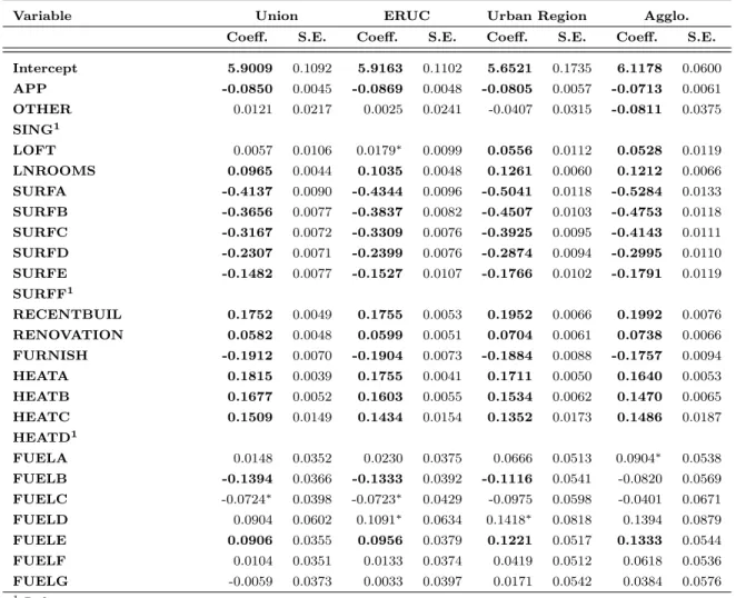
For the dwelling structural characteristics, most of the results are as expected. The value of a dwelling increases with its number of rooms and its surface. Renovated dwellings and dwellings recently built have higher monthly rents. Dwellings with central heating (especially those with individual central heating) are dearer than those with other heating installations. Dwellings using coal or wood as the source of energy for heating are less expensive. This is not surprising since heating with coal or wood is an indicator of the poor quality of a dwelling (Vannesteet al., 2007). Dwellings using electricity as the source of energy are more expensive. Dwellings with bathrooms, toilets, double glazing, and wall isolation are more valuable. Moreover, the more garage places a dwelling has, the more expensive it is. All other things being equal, apartments are cheaper than single-family houses.
Other results are more puzzling. Studios and lofts are, ceteris paribus, more expensive than other dwellings. Furnished dwellings are less expensive. While this may seem paradoxical, this can be due to the fact that this category of dwellings targets mostly low-income categories such as students who cannot afford to furnish and to renovate their dwellings.
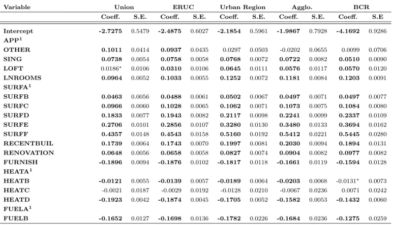
Most of the results about environmental quality variables and neighborhood attributes are in line with expectations. Rental prices are low when the pollution indicator is high. This is not surprising since we expect greater demand for dwellings located in less polluted areas. The coefficient of LNSLOPE (AC) is positive. This confirms the assumption that hilly landscapes are more attractive to residents.9 The coefficient obtained for the variableLNPERFOR (AC)is
8We chose the specification in Table 8, which uses the potential accessibility to jobs as a measure of accessibility,
by comparing several alternative models in Table 4 in Appendix D in terms of goodness of fit criteria (AIC and SBC). In Table 4, our preferred specification is displayed in column (2). It outperforms the corresponding semilog specification shown in column (1). Moreover, it has a better fit than models in the column (3) and the column (4) where the proxies of accessibility are respectively the density of population and the Harris Market Potential. While the density of population is not a “natural” measure of accessibility, it is significantly correlated with the potential accessibility to jobs (the pairwise correlation between LNPOT JOBS and LNDENS POPis significant and equal to 0.7713). Therefore, due to multicollinearity, simultaneously inserting the potential accessibility to jobs and the density of population yields a non significant coefficient forLNDENS POP.
9Goffette–Nagotet al. (2011) test this assumption by estimating a hedonic regression with data collected at the
positive and significant. This indicates that dwellings located in neighborhoods covered by forests are sought-after. The results obtained with theLNSLOPE (AC)and theLNPERFOR (AC)
variables are clearcut. They emphasize that households value positively neighborhoods with environmental amenities.
The sign of the LNPERAR (AC) coefficient is more difficult to interpret; it suggests that dwellings located in neighborhoods largely covered by agriculture are less valuable. This may indicate that such neighborhoods are deprived of infrastructures and amenities (schools, shop-ping centers, etc.) that are required by most households or that agriculture entails some negative neighborhood externalities. Dwelling rents increase with LNPOT JOBS the indicator of po-tential accessibility to jobs, which suggests that there is a greater demand for more accessible residential areas.10 Finally, the coefficient of the variable LNMEDINC is positive and signifi-cant, indicating that dwellings located in wealthy neighborhoods are more expensive.
Insert Table 8 about here.
Table 8 shows the impact of the choice of the limits of the agglomeration on econometric results through estimations of separate samples. The econometrics literature recommends rather to perform an estimation with interaction terms based on the largest sample. This procedure has the advantage of testing whether each coefficient varies significantly, in a statistical viewpoint, across different delineations. However, as it adds to the previous specification several interaction terms that are likely to be correlated with the other regressors, this procedure has the potential shortcoming of increasing the multicollinearity between regressors. Table 5 in Appendix E shows that several interaction terms are significant which clearly imply that the coefficients of several regressors vary significantly across different definitions of the study area.11 This further confirms
the sensitivity of statistical results to the delineation of the study area.
The use of household data helps greatly to improve the results regarding this variable.
10Results for theLNPERAR (AC)and the LNPOT JOBSwill be challenged in the two-stage estimation
approach where we control for endogeneity.
11Considering specifically the elasticity of potential accessibility and of its interaction terms, we find an elasticity
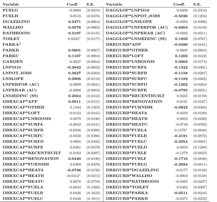
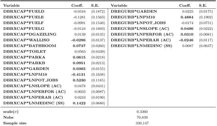
of 0.3627 for the Union area and of 0.5230 forDBRXCAP*LNPOT JOBS — the interaction term between potential accessibility to jobs and the dummy depicting the pertainance of a dwelling to Brussels Capital Region — and of -0.5026 for DAGGLOP*LNPOT JOBS — the interaction term between potential accessibility to jobs and the dummy related to the agglomeration macrozone. Therefore, the implied elasticities for the Union area, Brussels Capital Region, and the Operational Agglomeration delineation are respectively 0.3627, 0.8857 and -0.1399. We can note that the corresponding results in Table 8 are respectively 0.3548, 0.3663 and 0.1917. While the ordering of the elasticities remains the same, the model with interaction terms overestimate the elasticity of potential accessibility for the Union area and Brussels Capital Region and underestimate it for the agglomeration macrozone. Therefore, the multicollinearity caused by the addition of interaction terms is likely to affect the precision of the estimates.
To sum up, choices regarding the limits of the study area are not benign regarding econo-metric results. The reason of those discrepancies may lie on a spatial heterogeneity argument. The different delineations imply distinct geographic structures: the larger the study area, the larger will be the implied proportion of rural hinterland; which is by nature less urbanized and less accessible from the main centers of activities and employment. Therefore, the choice of the study area is a very sensitive issue regarding the precision of estimates. This further stresses the need to delineate the study area in a way that is consistent with the problem under in-vestigation. A failure to do so would entail biases that may mislead statistical inferences and the policy recommendations that they may drive. For instance, the elasticity of the potential accessibility indicator rises from 0.1917 for the Operational Agglomeration macrozone to 0.3663 for the Brussels Capital Region, which implies a 91% increase. Such a discrepancy may lead to highly mistaken conclusions in terms of land use and transport policies. Magrini (2004) warns against the measurement problems resulting from the mismatch between the spatial pattern of the process under study and the boundaries of the observational units. In the specific context of regional convergence analysis, the inadequate choice of the observational units might hide sub-stantial dependence of income growth. However, Magrini’s claim does not specifically concern the limits of the study area, but rather those of the basic spatial units. In the next subsection, we specifically address the question of the choice of basic spatial units.
5.1.2 Impacts of the choice of the basic spatial unit
After having evidenced that statistical results are sensitive to the delineation of the study area, we now investigate the impact of the aggregation scale on econometric findings. Briant et al.
(2010) assess the impact of size and shape distortions on the behavior of simple regression co-efficients. Concerning the size distortion, they find that if the aggregation distortion on the explanatory variables and the dependent variable are similar, the size effect of the MAUP will be small. Such a condition holds when both the explanatory and dependent variables are spatially autocorrelated and averaged. The size issue is more disturbing when the dependent and the explanatory variables are not aggregated by the same process or do not display the same level of spatial autocorrelation. Our dependent variable and the dwellings structural attributes are indi-vidual characteristics. Therefore, in our analysis aggregation biases concern only environmental and neighborhood variables.
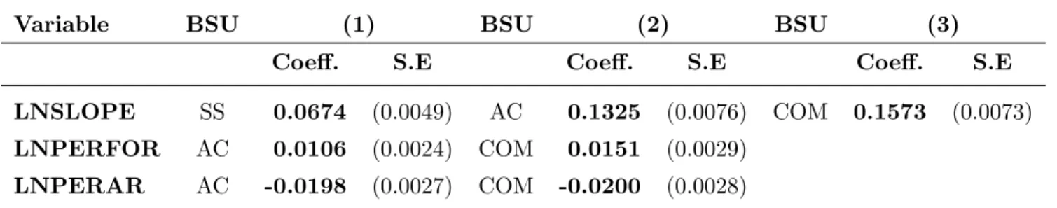
Table 9 compares estimation results when the median income by tax declaration is measured successively at the statistical sector and at the municipal levels while Table 10 compares coef-ficient estimates when the average income by tax declaration is measured successively at the statistical sector, the former township and at the municipal levels. They show that the
coeffi-cients of the logarithm of the median and average income are higher when the scale of measure of those variables is higher. Similar results are obtained for other neighborhood and environmental variables as shown in Table 6 in Appendix F.
Such results are consistent with Gehlke and Biehl (1934) findings which outline that the correlation coefficient tends to increase as the size of spatial units increases. What is the rationale of such findings? A possible explanation may be the following: the larger the BSU, the lower the variance of a variable. Since the standard deviations of variables lie in the denominator of the correlation coefficient and the simple regression coefficient this may explain their increase when the size of a BSU increases. We may conjecture that a similar effect operates on variable coefficients in the interval regression model.
Insert Table 9 about here.
Changing the scale of the basic spatial unit for one variable also impacts the coefficients of the other variables. In Table 9, the most important effects are observed in the intercept, which is more than twice as large in the second specification, in the GARDEN coefficient, which is not significant in the first specification and more than twice as large in the second specification, and in the LNPM10 coefficient which is not significant in the second specification.12
In Table 10, we also observe substantial changes in the intercept, which is more than doubled from the first to the third specification, the GARDEN coefficient, which is not significant in the first specification but increases by almost 50% from the second to the third specification, and the LNPM10 coefficient, which is not significant in the second specification and is positive — a surprising result — in the third specification. Therefore, the intercept, the garden and the pollution variables’ coefficients appear as very sensitive to changes in the size of the basic spatial units.
Insert Table 10 about here.
The results just described outline the necessity of using the finest spatial scale for the definition of environmental quality and neighborhood attributes. Using larger basic spatial units for the definition of those variables would result in inflated estimates. Once more, such biases may imply misleading conclusions in terms of the policy recommendations drawn from econometric results. However, due to constraints in data availability, sometimes they are unavoidable as the information of some variables may only be obtained at specific spatial scales. This is precisely the case with the pollution indicator which, because of raster resolution, can only be computed at the municipal level. In such cases of spatial scale constraints, one should be aware of the potential biases.
Using inappropriate spatial scales may trigger endogeneity of the “error in variables” kind. In the case of a continuous dependent variable, Anselin and Lozano–Gracia (2008) use a Spatial 2SLS method to handle both spatial dependence and endogeneity generated by spatial interpolation of air quality values. While this approach may be relevant for handling biases due to spatial scales in cases where the regressand is continuous, it is tremendously challenging in the interval regression context. However, it may be considered in the second stage of the two-step procedure with locational fixed effects and deserves to be explored in future contributions.
5.2
Spatial Interval regression models
Let us now investigate the substantive spatial dependence issue through a Spatial Autoregressive Interval Regression (SARIR) model, a Spatial Durbin Interval Regression model (SDMIR) and a General Spatial Interval Regression (SACIR) model. We have not been able to run those spatial models algorithms on the full dataset. Indeed, they are very demanding in terms of computational resources. So we ran those algorithms on two subsamples of respectively 2,969 observations and 62 statistical sectors (Sample 1) and 2,565 observations and 81 statistical sectors (Sample 2).13
Dwellings of Sample 1 are located in the municipalities of Anderlecht, Berchem-Sainte-Agathe, and Molenbeek-Saint-Jean. The geographical locations of Sample 2 dwellings lie within the municipalities of Auderghem, Woluwe-Saint-Lambert, and Woluwe-Saint-Pierre.14 Figures 2 and
3 depict the average income in Brussels Capital Region (BCR) as well as the location of Sample 1 and Sample 2 dwellings in the BCR.
Unfortunately, there is not enough variation in the environment and neighborhood attributes to assess reliably any potential impact of changes of the basic spatial unit. Table 11 displays the results of the basic interval regression model as well as those of the SARIR, the SDMIR and the SACIR algorithms. The SDMIR and the SACIR models seem less credible than the SARIR model because the disturbance spatial dependence parameter λ and the coefficients of
13All our Gibbs sampler algorithms are written in GAUSS 12. They imply 2,500 draws with an initial 500
draws “burn-in” sequence for the SAR and the SDM algorithms, and an initial 1000 draws “burn-in” sequence for the SAC algorithm. For a 2,969 observations sample, the SAR algorithm takes a total time of about 3 days, 11 hours, 39 minutes and 54 seconds on a Dell Precision workstation with a 64 GB RAM and with 2 processors of respectively 2.80 GHz and 2.79 GHz processor speed.
14Considering an axis dividing Brussels Capital Region from the South-East to the North-East, then the first
sample lies in the part of Brussels above that axis and the second sample in the other side. As shown in Figure 2, most of the municipalities of Brussels above that axis, like Moleenbeek-Saint-Jean, Anderlecht and Saint-Josse have a lower average income (Ganshoren, Berchem-Sainte-Agathe, and Jette are exceptions characterized by higher incomes). Municipalities below that axis, especially Uccle, Watermael-Boitsfort, Auderghem and Woluwe-Saint-Pierre have a higher average income.
the regressors spatial lags are not significant. One has to be very cautious in comparing Interval Regression to SARIR, SDMIR and SACIR estimates. As for OLS, Interval Regression estimates have a straightforward interpretation as partial derivatives of the dependent variable with re-spect to an explanatory variable. Such an interpretation is possible because in the IR model the information set for an observation i contains only exogenous or predetermined variables associ-ated with observation i. In spatial models which contain spatial lags of the dependent variable, the interpretation of parameters becomes richer and more complicated (LeSage and Pace, 2009). Basically, such models allow a change in the explanatory variable for a single dwelling to poten-tially affect the dependent variable in all other dwellings. Therefore, the marginal effects in those models have a formal expression way more complex than in OLS settings (the formal expression of those marginal effects can be found in LeSage and Pace (2009, p.35-36)). In Table 11 we do not compare marginal effects of the regressors across non-spatial and spatial models, but rather their direct effects (i.e. the “true” effect of the regressors, after that spatial dependence has been accounted for (Kim et al., 2003).). The results of the IRM and the SARIR model differ substantially only for the spatial dependence parameter and the intercept. In the first sample estimations, the intercept is much lower in the spatial models than the one obtained in the bench-mark model. For the second sample, there appears to be a significant discrepancy in the intercept in the SACIR model, but not in the SARIR and SDMIR models. The substantial reduction of intercept in the SAR and SAC models may be an indication that the omitted-variable bias is significantly reduced in the spatial models.
Pace and LeSage (2010) establish that, in the presence of spatial dependence, non spatial models like OLS amplify omitted variable bias. Moreover, they show that estimates from the SDM model shrink the bias relative to OLS. In Appendix G, we show formally how the non spatial models compound this omitted variable bias.
Insert Figures 2 and 3 about here.
Omitting the spatial lag term, as in the non-spatial IRM, would definitely entail biased estimates. Such biases are perceptible in theLNMEDINC (SS)coefficient which is 17% higher in the non-spatial IRM estimation based on Sample 1 and 8% higher in the IRM estimation based on Sample 2 than in SARIR corresponding estimations. By acknowledging the impact of dwelling rents nearby in space, the spatial model implies a lower impact of the median income. Another noteworthy observation may be made about the LNMEDINC (SS) coefficient: it is the only coefficient of an environment or a neighborhood attribute that is significant for all specifications. As explained earlier, since the other environment and neighborhood variables are measured at a more aggregated level, they do not have sufficient variation to allow enough precision in the
measure of their estimates.
Another interesting result lies in the discrepancy between Sample 1 and Sample 2 SARIR model results. For instance, the spatial dependence parameter and the LNMEDINC (SS) co-efficient are higher for Sample 2 than for Sample 1. Those results indicate that the neighborhood has a stronger impact in the determination of Sample 2 dwelling rents than in Sample 1. The difference between Sample 1 and Sample 2 results yields some evidence of spatial heterogeneity in the estimation. Spatial heterogeneity is related to the lack of stability over space of the relation-ship under study. It implies that functional forms and parameters vary with location (Anselin, 1988).
Insert Table 11 about here.
5.3
Two-stage estimation with locational fixed effects
While the SARIR model may mitigate the omitted variable bias by inserting a spatial lag term, it does not control for the endogeneity generated by the simultaneous causality between the dwelling rents and the observed locational characteristics, like the average income. Indeed, while we may expect dwelling rents to be high as a resultant of high average income in the area, we may as well consider areas with high dwelling rents as a sign of attractiveness for high-income households because they are expected to host better schools or because they host socio-economic peers. Since reverse causality is more likely to concern location invariant attributes, the two-step estimation procedure address this endogeneity problem by retrieving locational fixed effects at the first step.
Insert Table 12 about here.
Table 7 in Appendix H provides results for the first stage. They are as expected and in line with the previous estimations. Before discussing the effects of a choice of a specific delineation, few remarks are in order. The first one is that conversely to earlier results where the percentage of the basic spatial unit covered by agriculture had a negative impact on dwelling rents while potential accessibility had a positive elasticity, Table 12 indicates reverse effects for those two variables. The private dwelling market of the Brussels Metropolitan area values dwellings close to agricultural areas and with a lower accessibility to the main employment centers. Clearly, inconveniences of urban life (congestion, pollution etc.) reflect in marginal prices.
Insert Table 13 about here.
Moreover, the SAC model is validated in this second-step estimation for the Urban Region and the ERUC samples since we obtain significant disturbance spatial dependence parameters. It
provides more precise estimations (lower mean square error) and a better fit (Higher Pseudo ¯R2).
As before, choices of delineation impact statistical results. From the agglomeration to the Union samples, we obtain different estimates. This holds for OLS and spatial specifications. Therefore, controlling for substantive spatial dependence does not mitigate bias due to the delineation choices. This further highlights the necessity to delineate the study area consistently.
Regarding the impact of the choice of the basic spatial unit, the second-step estimation provides outcomes that are similar to the results obtained with the Interval Regression Model. Table 13 compares results when the median income by tax declaration is measured successively at the statistical sector and at the municipal levels. It confirms that the coefficient of the logarithm of the median income is higher when average income is measured at the municipal level.
6
Conclusion
Microsimulation tools require a massive amount of geocoded data, collected from several sources and often available at different spatial scales. Hence, choices have to be made about the rel-evant underlying basic spatial units (BSU), as well as the limits of the studied area. Those choices are generally suspected to influence or even bias econometric results. Moreover, spatial autocorrelation is also likely to have significant impact on statistical findings.
The goal of this paper was to address those issues by carrying out sensitivity analyses. There-fore, on the basis of the hedonic regression model, we have investigated the three aforementioned problems.
The delineation of the metropolitan area highly impacts the statistical estimations. We show that most of the coefficients vary significantly with the definition of the study area. Hence, defining a city by functional or morphological criteria, as each urban specialist or planner would do, will lead to different results to that defined by a transportation regional planner.
A second spatial aspect addressed by this paper is the choice of the basic spatial units. The sensitivity of the coefficients to scale effect is empirically demonstrated on the example of Brussels. Our results are consistent with Gehlke and Biehl (1934) and the related literature. A possible explanation of such findings is that the larger the size of the BSUs, the lower the variance of the considered variable.
Therefore, in order to minimize the biases, the delineation of the study area must be chosen in a way that is consistent with the phenomenon under investigation. Moreover, the finer the aggregation scale, the more precise the coefficient estimates. Indeed, bad choices in terms of the aggregation scale may lead to misspecification biases. In the ideal situation where all the statistical information is available at the individual level, biases inherent to the ecological fallacy would not exist.
We also accounted for the impact of substantive spatial dependence. As we obtained a statistically significant spatial dependence parameters from those estimations, our econometric results provide evidence of spatial dependence. The estimation of these spatial econometric models is likely to mitigate the omitted-variable bias which generally undermines traditional hedonic estimation.
However, the preceding approaches are “naive” in the sense that they do not address the endogeneity biases inherent to the hedonic regression model. To face this shortcoming, we apply a two-step estimation procedure with locational fixed effects. This estimation strategy shows that, while the explicit consideration of spatial effects in the econometric specification improves the fit of the model, it is still vulnerable to biases due to choices in terms of either the delineation
of the study area or the basic spatial unit.
Conversely to the previous approaches for which we obtained a negative elasticity for the percentage of the basic spatial unit covered by agriculture and a positive elasticity for the po-tential accessibility, this method implies opposite effects for those two variables. This suggests that dwellings close to agricultural areas and with a lower accessibility to the main employment centers are sought-after and that endogeneity biases are not negligible.
Other results from this two-step estimation procedure further confirm previous findings. Therefore, even more attention should be paid to issues related to nuisance spatial dependence and to spatial heterogeneity. The future implementations of microsimulation models in the field of transportation and spatial planning should take that into consideration in order to avoid compounding all kinds of spatial biases.
Eventually, this contribution outlines two interesting research perspectives. The discrepancy between Sample 1 and Sample 2 SARIR estimation results provides strong evidence of spatial heterogeneity. Therefore, one could consider performing a careful investigation of that issue while addressing concomitantly endogeneity issues. Moreover, it would be interesting to use Spatial 2SLS for attempting to mitigate biases arising from choices of the spatial scale.
Acknowledgements. This research was conducted when the first author was appointed at CORE (UCLouvain) in the framework of the EU project named Sustaincity. We are grateful to all WP leaders and members of this project for their fruitful remarks. Special thanks are also addressed to Luc Bauwens and the anonymous referees for their valuable comments and suggestions on an earlier version of this paper. The usual disclaimer applies.
App
endix
A:
Descriptiv
e
statistics
of
con
tin
uous
v
ariables
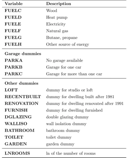
T able 1: Descriptiv e statistics (Sample:“Union”). V ariable Description N Min Max Mean S.D. dep enden t v aria ble LLNRENT ln of lo w er b ound of ren t in terv al 276,765 5.521 6.899 5.763 0.402 ULNRENT ln of up p er b ound of ren t in te rv al 309,615 5.521 6.899 6.211 0.338 Regressors LNR OOMS ln of n um b er of ro oms 305,161 0 4.595 1.215 0.532 LNPM10 ln of a v erage concen tration of PM 10 b y m unicipalit y 330,147 3.221 3.601 3.445 0.088 LNPERF OR (COM) ln(P ERF OR+1) b y m unicipalit y 330,147 0 4.034 0.989 1.184 LNPERF OR (A C) ln(PERF OR+1) b y former to w n sh ip 330,118 0 4.035 0.847 1.204 LNPERAR (COM) ln(PERAR+1) b y m unicip alit y 330,147 0 4.472 2.123 1.775 LNPERAR (A C) ln(PERAR+1) b y former to wnship 330,118 0 4.582 1.792 1.803 LNSLOPE (SS) ln(SLOPE) (b y statistical sector) 330,107 -0.680 2.945 1.012 0.523 LNSLOPE (A C) ln(SLOPE) (b y former to wnship) 330,118 -0.142 2.446 1.136 0.382 LNSLOPE (COM) ln(SLOP E) (b y m u nicipalit y) 330,147 0.049 1.876 1.132 0.353 LNMEDINC (SS) ln(MEDINC) (b y statistical sector) 326,038 9.126 10.595 9.817 0.158 LNMEDINC (COM) ln(MEDINC) (b y m unicipalit y) 330,147 9.570 10.104 9.830 0.112 LNA VINC (SS) ln(A VINC) (b y statistical sector) 300,366 9.458 10.947 10.053 0.208 LNA VINC (A C) ln(A VINC) (b y former to wnship) 326,335 9.646 10.665 10.085 0.163 LNA VINC (COM) ln(A VINC) (b y m unicipalit y) 330,147 9.756 10.574 10.102 0.149 LNDENS POP ln(DENS POP) (b y former to wnship) 330,118 3.673 9.862 7.926 1.365 LNPOT JOBS ln(POT JOBS) (b y former to wnship) 330, 11 8 12. 1 40 12. 9 48 12.693 0.179 LMARKPOT ln(MARKPOT) (b y former to wnship) 330,118 14.240 15.420 15.065 0.315App
endix
B:
Differen
t
limits
of
Brussels
T able 2: Num b er of observ ations (dw ellings) for eigh t differen t delineation s of Brussels. Spatial en tit y Description Nm un Nobs Brussels Capital Region (BCR) Administrativ e definition 19 177,721 Agglomeration Morphological agglomeration adjusted 36 208,371 to m u nicipalities b oundaries Urban region Agglomeration+Suburb 62 233,582 Residen tial ur ban complex Urban region+Residen tial Comm uting 122 283,079 (R UC) area Extended Residen tial Brussels R UC+Leuv en R UC 134 301,160 urban complex (E R UC) RER area Area serv ed b y the RER 135 314,279 Extended RER area RER area + 12 m u nicipalities 147 325,135 STRA TEC study area “Union” Municipalities p ertaining to 157 330,147 at least one delineation Nm un= n um b er of m u nicipalities, Nobs= n um b er of observ ations Source: V an Hec k e et al. (2009) and STRA TEC.¡
0 20 10 Ki lo m et er s Ca rto gr ap hy : A la in P HO LO B AL A, U CL , 2 01 0 Ex te nd ed R ER A re a Ag gl om er at io n Su bu rb Ex te nd ed re sid en tia l c om m ut in g ar ea Re gi on al B or de rs Bo rd er s of W al lo on a nd F le m ish B ra ba nt Figure 1: Differen t limits of Brussels a gglomerationAppendix C: List of dwelling structural characteristics
Table 3: List of variables linked to physical attributes of the dwellings.
Variable Description
Type of dwelling dummies
APP dummy for apartments
OTHER dummy for other kinds of dwelling
SING dummy for single family dwelling
Dwelling surface dummies
SURFA dwelling with a surface lower than 35 m2
SURFB dwelling with a surface between 35 and 54 m2
SURFC dwelling with a surface between 55 and 84 m2
SURFD dwelling with a surface between 85 and 104 m2
SURFE dwelling with a surface between 105 and 124 m2
SURFF dwelling with a surface higher or equal to 125 m2
Heating installation dummies
HEATA Individual central heating installation
HEATB Central heating installation common to several dwellings in one building
HEATC Central heating installation common to several dwellings in several buildings
HEATD Other heating installations
Dummies related to the composite quality index
QUALITY1 Insufficient quality
QUALITY2 Basic quality
QUALITY3 Good quality
QUALITY4 Good quality and spacious
QUALITY5 Very good quality
Dummies related to the source of energy used for heating
FUELA Fuel
FUELB Coal
Table 3 – concluded from previous page
Variable Description
FUELC Wood
FUELD Heat pump
FUELE Electricity
FUELF Natural gas
FUELG Butane, propane
FUELH Other source of energy
Garage dummies
PARKA No garage available
PARKB Garage for one car
PARKC Garage for more than one car
Other dummies
LOFT dummy for studio or loft
RECENTBUILT dummy for dwelling built after 1981
RENOVATION dummy for dwelling renovated after 1991
FURNISH dummy for dwelling furnished
DGLAZING double glazing dummy
WALLISO wall isolation dummy
BATHROOM bathroom dummy
TOILET toilet dummy
GARDEN garden dummy
Appendix D: Estimation results for various proxies of
ac-cessibility
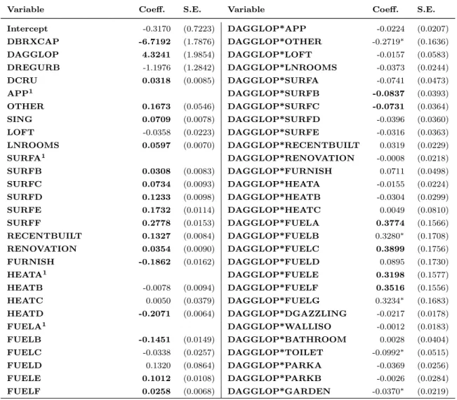
Table 4: Interval regression: estimation results for various proxies of accessibility (Sample: Union).
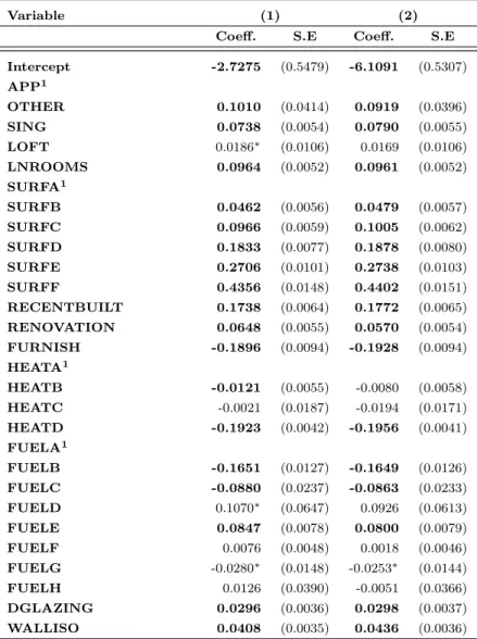
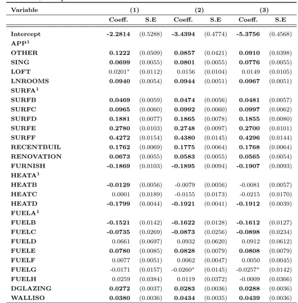
Variable (1) (2) (3) (4)
Coeff. S.E Coeff. S.E Coeff. S.E Coeff. S.E
Intercept 4.6916 (0.0812) -2.7275 (0.5479) 1.0568 (0.3362) -1.2290 (0.5392) APP1 OTHER 0.0965 (0.0413) 0.1011 (0.0414) 0.0991 (0.0415) 0.0994 (0.0414) SING 0.0702 (0.0056) 0.0738 (0.0054) 0.0674 (0.0054) 0.0736 (0.0055) LOFT 0.0188∗ (0.0106) 0.0186∗ (0.0106) 0.0183∗ (0.0106) 0.0199∗ (0.0104) LNROOMS 0.0964 (0.0052) 0.0964 (0.0052) 0.0952 (0.0053) 0.0965 (0.0052) SURFA1 SURFB 0.0474 (0.0056) 0.0463 (0.0056) 0.0452 (0.0056) 0.0450 (0.0056) SURFC 0.0983 (0.0060) 0.0966 (0.0060) 0.0960 (0.0059) 0.0955 (0.0060) SURFD 0.1854 (0.0078) 0.1833 (0.0077) 0.1837 (0.0077) 0.1823 (0.0076) SURFE 0.2726 (0.0102) 0.2706 (0.0101) 0.2713 (0.0102) 0.2702 (0.0101) SURFF 0.4376 (0.0150) 0.4357 (0.0148) 0.4397 (0.0150) 0.4362 (0.0148) RECENTBUILT 0.1716 (0.0061) 0.1739 (0.0064) 0.1705 (0.0064) 0.1736 (0.0066) RENOVATION 0.0651 (0.0056) 0.0648 (0.0056) 0.0644 (0.0056) 0.0647 (0.0056) FURNISH -0.1918 (0.0095) -0.1896 (0.0094) -0.1911 (0.0095) -0.1879 (0.0094) HEATA1 HEATB -0.0110 (0.0056) -0.0121 (0.0055) -0.0141 (0.0054) -0.0106∗ (0.0055) HEATC -0.0016 (0.0186) -0.0021 (0.0187) -0.0057 (0.0188) -0.0025 (0.0187) HEATD -0.1925 (0.0043) -0.1923 (0.0042) -0.1956 (0.0044) -0.1943 (0.0042) FUELA1 FUELB -0.1675 (0.0127) -0.1652 (0.0127) -0.1655 (0.0127) -0.1648 (0.0127) FUELC -0.0903 (0.0238) -0.0880 (0.0238) -0.0847 (0.0234) -0.0875 (0.0237) FUELD 0.1001 (0.0639) 0.1070∗ (0.0647) 0.1008 (0.0642) 0.1096∗ (0.0645) FUELE 0.0820 (0.0080) 0.0847 (0.0078) 0.0858 (0.0081) 0.0879 (0.0079) FUELF 0.0028 (0.0050) 0.0076 (0.0048) 0.0118 (0.0050) 0.0134 (0.0049) FUELG -0.0275∗ (0.0149) -0.0281∗ (0.0148) -0.0270∗ (0.0149) -0.0291∗ (0.0149) 1Reference case.
Bold: significant at 0.05 level.
*significant at 0.10 level.
Table4 – concluded from previous page
Variable (1) (2) (3) (4)
Coeff. S.E Coeff. S.E Coeff. S.E Coe