Quantile Based Estimation of Scale and Dependence

This thesis must be used in accordance with the provisions of the Copyright Act 1968.

Reproduction of material protected by copyright may be an infringement of copyright and

copyright owners may be entitled to take legal action against persons who infringe their copyright.

Section 51 (2) of the Copyright Act permits an authorized officer of a university library or archives to provide a copy (by communication or otherwise) of an unpublished thesis kept in the library or archives, to a person who satisfies the authorized officer that he or she requires the reproduction for the purposes of research or study.

The Copyright Act grants the creator of a work a number of moral rights, specifically the right of attribution, the right against false attribution and the right of integrity.

You may infringe the author’s moral rights if you: - fail to acknowledge the author of this thesis if

you quote sections from the work - attribute this thesis to another author - subject this thesis to derogatory treatment

which may prejudice the author’s reputation For further information contact the University’s Director of Copyright Services

D E P E N D E N C E

g a r t h ta r r

A thesis submitted in fulfilment of the requirements for the degree of

Doctor of Philosophy

School of Mathematics and Statistics Faculty of Science

University of Sydney 19 May 2014

which can always be made precise. — John Wilder Tukey (1962)

The sample quantile has a long history in statistics. The aim of this thesis is to explore some further applications of quantiles as simple, convenient and robust alternatives to classical procedures. The first application we con-sider is estimating confidence intervals for quantile regression coefficients, however, the core of this thesis is the development of a new, quantile based, robust scale estimator and its extension to autocovariance estimation in the time series setting and precision matrix estimation in the multivariate set-ting.

Chapter 1 addresses the need for reliable confidence intervals for quantile regression coefficients particularly in small samples. The existing methods for constructing confidence intervals tend to be based on complex asymp-totic arguments and little is known about their finite sample performance. We consider taking xy-pair bootstrap samples and calculating the corres-ponding quantile regression coefficient estimates for each sample. Instead of estimating a covariance matrix based on these bootstrap samples, our ap-proach is to take the appropriate upper and lower quantiles of the bootstrap sample estimates as the bounds of the confidence interval. The resulting confidence interval estimate is not necessarily symmetric; only covers ad-missible parameter values; and is shown to have good coverage properties. This work demonstrates the competitive performance of our quantile based approach in a broad range of model designs with a focus on small and moderate sample sizes. These results were published in Tarr (2012).

A reliable estimate of the scale of the residuals from a regression model is often of interest, whether it be parametrically estimating confidence in-tervals, determining a goodness of fit measure, performing model selection, or identifying unusual observations. The robustness of quantile regression parameter estimates to y-outliers does not extend to the error distribution – extreme observations in the y space yield outlying residuals which can interfere with subsequent analyses. This led us to consider the more funda-mental issue of robust estimation of scale.

Chapter 2 forms the core of this thesis with its investigation into robust es-timation of scale. Common robust estimators of scale such as the interquart-ile range (IQR) and the median absolute deviation from the median (MAD) are inefficient when the observations come from a Gaussian distribution.

scale estimator, Pn, which is proportional to the IQRof the pairwise means.

The estimator Pn is the scale analogue of the Hodges-Lehmann estimator

of location, the median of the pairwise means. When the underlying dis-tribution is Gaussian, the Hodges-Lehmann estimator is considerably more efficient than the median however it is not as robust – similarly, Pn trades

some robustness for significantly higher Gaussian efficiency.

In the theoretical treatment, Pn is considered as a special case of a more

general class of estimators – based on the difference of two quantiles of the pairwise means. For this class of estimators, assuming the observations are independent and identically distributed, we show that the influence func-tion is bounded and establish asymptotic normality.

Further extensions to Pn incorporate adaptive trimming to achieve the

maximal breakdown value of 50%. The resulting adaptively trimmed scale estimator has enhanced performance at extremely heavy tailed distributions and is shown to be triefficient across Tukey’s three corner distributions amongst the set of estimators considered. The adaptively trimmed Pn also

yields good results in the multivariate setting discussed in Chapter 4

The primary advantage of Pn over competing estimators is its high

effi-ciency at the Gaussian distribution whilst maintaining desirable robustness and efficiency properties at moderately heavy tailed and contaminated dis-tributions. The desirable efficiency properties of Pn are shown to be even

more marked over competing scale estimators in finite samples. The results of this chapter have been published in Tarr, Müller and Weber (2012) and presented at ICORS 2011.

Chapter 3 extends our robust scale estimator to the bivariate setting in a natural way as proposed by Gnanadesikan and Kettenring (1972). In do-ing so we move from estimatdo-ing scale to estimatdo-ing dependence. We show that the resulting covariance estimator inherits the robustness and efficiency properties of the underlying scale estimator.

Motivated by the potential to extend the efficiency and robustness proper-ties of Pn to the time series setting, Chapter 3 also considers the problem of

estimating scale and autocovariance in dependent processes. We establish the asymptotic normality ofPn under short and mildly long range

depend-ent Gaussian processes. In the case of extreme long range dependence, we prove a non-Gaussian limit result for theIQR, consistent with results found previously for the sample standard deviation and Qn. In contrast with the

terms in the Bahadur representation of Wu (2005). Simulation suggests that an equivalent result holds for Pn; we state the conjectured result which will

require the analogous Bahadur representation for U-quantiles under long range dependence. It is reasonably straightforward to extend the asymptotic results for the robust scale estimator to the corresponding robust autocov-ariance estimators. Various results from this chapter have been presented at ASC 2012 and EMS 2013.

Classical robust estimators assume that contamination occurs within a subset of the observations, however in recent years there has been interest in developing robust estimators that perform well under scattered contam-ination. Chapter 4 looks at the problem of estimating covariance and preci-sion matrices under cellwise contamination. A pairwise approach is shown to perform well under much higher levels of contamination than stand-ard robust techniques would allow. Rather than using the Orthogonalised Gnanadesikan and Kettenring procedure (Maronna and Zamar, 2002), we consider a method that transforms a symmetric matrix of pairwise cov-ariances to the “nearest” covariance matrix (in a Frobenius norm sense). We combine this method with various regularisation routines purpose built for precision matrix estimation. This approach works well with high levels of scattered contamination and has the advantage of being able to impose sparsity on the resulting precision matrix. Some preliminary results from this chapter have been presented at ICORS 2013.

Some of the ideas and figures from the first two chapters of this thesis have appeared in the following publications:

Tarr, G., Müller, S., and Weber, N. C. (2012). A robust scale estimator based on pairwise means. Journal of Nonparametric Statistics,24(1), 187–199. Tarr, G. (2012). Small sample performance of quantile regression

confid-ence intervals. Journal of Statistical Computation and Simulation, 82(1), 81–94.

A number of the results have been presented at the following conferences: Robust scale and autocovariance estimation. European Meeting of

Statisti-cians, 2013, Budapest, Hungary.

Robust covariance estimation via quantiles of pairwise means and applic-ations. International Conference on Robust Statistics, 2013, St Petersburg, Russia.

Robust scale estimation with extensions.Young Statisticians Conference, 2013, Melbourne, Australia.

Robust covariance estimation with Pn.Australian Statistical Conference, 2012,

Adelaide, Australia.

Efficient and robust scale estimation.International Conference on Robust Stat-istics, 2011, Valladolid, Spain.

Seminar presentations have been given at the following universities:

Robust estimation of scale and covariance with Pn and its application to

principal components analysis. University of NSW, School of Mathem-atics and Statistics, 2013, Sydney, Australia.

Robust estimation of scale and covariance with Pn and its application to

precision matrix estimation. University of Sydney, School of Mathem-atics and Statistics, 2013, Sydney, Australia.

I have been fortunate to have the unfailing support of a number of very talented and generous people over my time at the University of Sydney and the last four years in particular.

Firstly, to Neville Weber and Samuel Müller, I could not have asked for more dedicated, patient and knowledgable supervisors. Their complement-ary skills have led to an interesting and varied thesis. Neville’s breadth of statistical and probabilistic understanding and his expertise in asymptotic arguments gave me the impetus and courage to continue to push outside my comfort zone. Samuel’s initial idea for the new scale estimator gave rise to the core of the thesis and his background in robustness provided inspira-tion for new direcinspira-tions.

Their fanatical/rigorous/enthusiastic/fervent/dogged/rabid attention to detail lead to significant improvements in clarity and structure. They helped make me a better statistician and a better communicator. Though after suf-fering through many years of grammatical abuse, I fear I may have worn down Neville’s resolve against the split infinitive.

I have been extremely lucky to have had many travel opportunities to net-work and peddle my statistical wares. I am grateful for the financial support I received from the University of Sydney’s Postgraduate Research Support Scheme, the School of Mathematics and Statistics’ statistics research group, the Statistical Society of Australia through their Golden Jubilee Travel Grant and my supervisors.

I also want to thank my fellow PhD candidates, colleagues and students at the University of Sydney for making it an enjoyable few years. Ellis Patrick and Emi Tanaka who shared the journey with me from the beginning; many coffees with Justin Wishart, Patrick Noble, Luke Cameron-Clarke and Kellie Morrison; discussions at Hermanns with Michael Stewart, John Ormerod, Lisa Cameron and more recently Sanjaya Dissanayake, Tom Porter and Shila Ghazanfar.

My eternal gratitude goes to my partner Georgie Philpott and my parents for their support and for defending me when my grandmother invariably asks why I am still at university.

1 q ua n t i l e r e g r e s s i o n c o n f i d e n c e i n t e r va l s 1

1.1 Introduction 1

1.2 Overview of confidence interval construction techniques 3

1.2.1 Direct estimation 4

1.2.2 Rank inversion 4

1.2.3 Resampling methods 5

1.3 Simulation study 7

1.3.1 Heavy tailed errors 8

1.3.2 Skewed covariates 11

1.3.3 Multiple regression and heteroskedasticity 12

1.4 Conclusion 17

2 s c a l e e s t i m at i o n 19

2.1 Introduction 19

2.2 Background theory 21

2.2.1 U- andU-quantile statistics 21 2.2.2 Generalised L-statistics 23

2.3 Review of robust scale estimation theory 24

2.3.1 Measures of robustness 24

2.3.2 Existing scale estimators 26

2.4 A scale estimator based on pairwise means 32 2.4.1 The estimator Pn 32

2.4.2 Properties of Pn 37

2.5 Relative efficiencies in finite samples 42

2.5.1 Design 43

2.5.2 Results 44

2.6 Conclusion 49

3 c ova r i a n c e a n d au t o c ova r i a n c e e s t i m at i o n 51

3.1 Introduction 51

3.2 Robust covariance estimation 52

3.2.1 Properties 53

3.2.2 Simulations 56

3.3 Robust autocovariance estimation 61

3.4 Short range dependent Gaussian processes 64 3.4.1 Results for Pn 64

3.4.2 Results for ˆγP(h) 68

3.5 Long range dependent Gaussian processes 70

3.5.1 Parameterisation 73

3.5.2 Hoeffding versus Hermite decomposition 74 3.5.3 Interquartile range 76 3.5.4 Results for Pn 80 3.5.5 Results for ˆγP(h) 88 3.6 Simulations 92 3.7 Conclusion 97 4 c ova r i a n c e a n d p r e c i s i o n m at r i x e s t i m at i o n 100 4.1 Introduction 100 4.2 Scattered contamination 102 4.3 Performance indices 105 4.3.1 Matrix norms 105 4.3.2 Other indices 107

4.3.3 Behaviour of performance indices 110 4.4 Pairwise covariance matrix estimation 116

4.4.1 OGK procedure 116

4.4.2 NPD procedure 118

4.4.3 Comparing OGK and NPD 119

4.5 Precision matrix estimation 121

4.5.1 GLASSO 122 4.5.2 QUIC 122 4.5.3 CLIME 124 4.6 Simulation study 125 4.6.1 Design 125 4.6.2 Results 127 4.7 Conclusion 137 Appendices 138 a q ua n t i l e r e g r e s s i o n c o n f i d e n c e i n t e r va l s 139 b s c a l e e s t i m at i o n 145

b.1 Finite sample correction factors 145 b.2 Implosion breakdown 147

b.3 Pairwise mean scale estimator code for R 148 b.4 EM algorithm implementation 149

c c ova r i a n c e a n d au t o c ova r i a n c e e s t i m at i o n 151 c.1 Technical results 151

c.1.1 Hadamard differentiability 151 c.1.2 Influence functions 151

c.2 Hermite ranks 152

c.2.1 Influence function of P_n 152

c.2.2 Empirical distribution function 154 c.2.3 Pairwise mean distribution function 155 c.3 Results for SRD processes 158

c.3.1 Convergence of empirical distribution functions 158 c.3.2 Central limit theorem 159

c.3.3 Existing results for estimators 159 c.4 Results for LRD processes 161

c.4.1 Limit results for U-processes 161 c.4.2 Existing results for estimators 164 c.5 Relative efficiencies 167

d c ova r i a n c e a n d p r e c i s i o n m at r i x e s t i m at i o n 168 d.1 Generating precision matrices 168

d.2 Entropy loss results 169 d.3 PRIAL results 172

d.4 Log determinant results 173 b i b l i o g r a p h y 174

Figure 1.1 The check function, ρτ(u) 4

Figure 1.2 Coverage probabilities for the heavy tailed error model 9 Figure 1.3 Average confidence interval lengths for the heavy tailed

error model 10

Figure 1.4 Coverage probabilities for the skewed covariate model 13 Figure 1.5 Average confidence interval lengths for the skewed

covariate model 14

Figure 1.6 Coverage probabilities for the multiple regression model with heteroskedasticity 16

Figure 2.1 Finite sample MADestimates 31

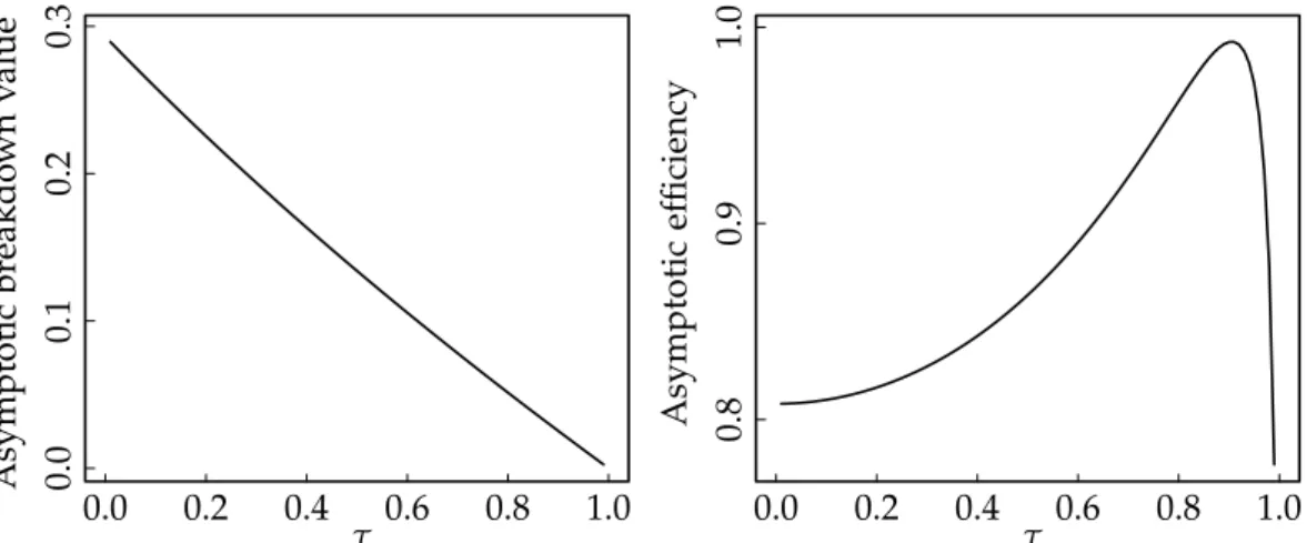
Figure 2.2 Breakdown value and efficiency ofPn(τ) 33

Figure 2.3 Finite sample relative efficiency of Pn(τ) 35

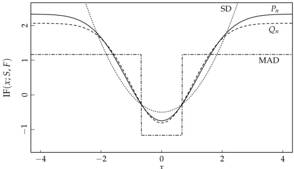
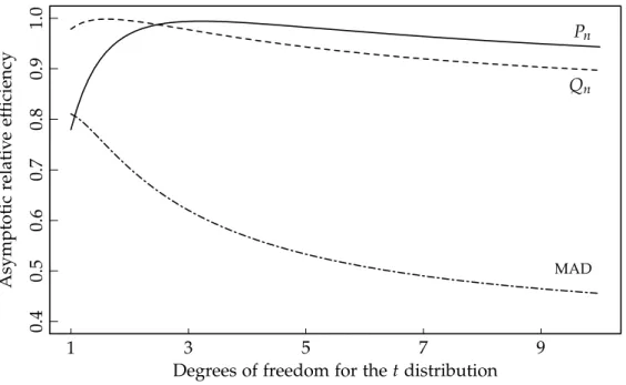
Figure 2.4 Influence functions at the Gaussian 39 Figure 2.5 Asymptotic relative efficiencies 40 Figure 2.6 Relative efficiencies att distributions 45

Figure 2.7 Relative efficiencies at Tukey’s three corners 46 Figure 3.1 Asymptotic variance of covariance estimators 55 Figure 3.2 Relative efficiency of robust correlation estimators over

varioust distributions 58

Figure 3.3 Relative MSEs of robust correlation estimators over varioust distributions 58

Figure 3.4 Efficiency of robust correlation estimators againstρ 60

Figure 3.5 MSEs of robust correlation estimators againstρ 60

Figure 3.6 Corruption and autocovariance estimators 62

Figure 3.7 Annual Nile river minima 71

Figure 3.8 ACFof the annual Nile river minima 72

Figure 3.9 ExampleLRDdata series 93

Figure 3.10 Empirical densities for scale estimates 96

Figure 3.11 Empirical densities for autocovariance estimates 98

Figure 4.1 Scattered contamination 103

Figure 4.2 Eigenvalue distortion 109

Figure 4.3 Covariance matrix performance indices 111 Figure 4.4 Precision matrix performance indices 111

Figure 4.5 Increasing variance and precision matrix elements 112

Figure 4.6 Increasing variance and the eigenvalues of precision

matrices 114

Figure 4.7 Scattered contamination and covariance matrices 115 Figure 4.8 Scattered contamination and precision matrices 115 Figure 4.9 PRIALresults for estimated covariance matrices under

moderate and extreme contamination 120

Figure 4.10 Precision matrix head maps 126

Figure 4.11 Example of the contaminating distribution 127 Figure 4.12 PRIALresults forCLIMEwith banded structures 130

Figure 4.13 PRIALresults for banded structures and p=60 132

Figure 4.14 PRIAL results for banded, scattered and dense preci-sion matrix structures with theQUICprocedure 133 Figure 4.15 Log determinant results for theGLASSOprocedure 135 Figure 4.16 Entropy loss and Frobenius norm results for

covari-ance matrices after usingCLIME 136

Figure A.1 Empirical coverage probabilities for the heavy tailed error model withn =100 140

Figure A.2 Empirical coverage probabilities for the heavy tailed error model withn =150 141

Figure A.3 Empirical coverage probabilities for the heavy tailed error model withn =200 142

Figure D.1 Entropy loss results forCLIMEwith extreme outliers 169 Figure D.2 Entropy loss results with extreme outliers 170

Figure D.3 Entropy loss results forQUICwith extreme outliers 171 Figure D.4 PRIALresults for moderate outliers 172

Table 2.1 Relative efficiencies at Tukey’s three corners 47 Table 2.2 Triefficiencies of various scale estimators 48

Table 3.1 MSEs underSRDprocesses 94

Table 3.2 Average estimates from an ARFIMA(0, 0.1, 0)process 95 Table 3.3 Average estimates from an ARFIMA(0, 0.4, 0) process 97 Table 4.1 PRIALresults when there is no contamination 128

Table A.1 Summary output for Cauchy distributed errors 143 Table A.2 Summary output for t3 distributed errors 143 Table A.3 Summary output for t5 distributed errors 144

Table A.4 Summary output for standard Gaussian errors 144

Table B.1 Finite sample correction factors 145

Table B.2 Sampling distribution of pairs 147

Table C.1 Efficiencies for ARFIMA(0, 0.1, 0) processes 167 Table C.2 Efficiencies for ARFIMA(0, 0.4, 0) processes 167

ACF autocorrelation function

CLIME constrained L1 minimisation for inverse covariance matrix estimation

CDF cumulative distribution function

CLT central limit theorem

GLASSO graphical lasso

IQR interquartile range

LRD long range dependent

MAD median absolute deviation from the median MCD minimum covariance determinant

MSE mean square error

MLE maximum likelihood estimate

NPD nearest positive definite

OGK Orthogonalised Gnanadesikan Kettenring

OGKw reweighted Orthogonalised Gnanadesikan Kettenring

PD positive definite

PRIAL percentage relative improvement in average loss

PSD positive semidefinite

QUIC quadratic inverse covariance

SD sample standard deviation

SRD short range dependent

e a small number

IF(x;T,F) influence function

bxc the integer part ofx

A| matrix transpose of A

I indicator function

S classical sample covariance matrix

Σ covariance matrix

Θ precision matrix

Φ standard Gaussian cumulative distribution function

φ standard Gaussian probability density function D −→ converges in distribution p −→ converges in probability ε proportion of contamination ε∗ breakdown value

F cumulative distribution function f probability density function Fn empirical distribution function

G cumulative distribution function of the kernels of aU-statistic Gn empirical distribution function of the kernels of aU-statistic

Hk kth Hermite polynomial

ui random error term

1

Q U A N T I L E R E G R E S S I O N C O N F I D E N C E I N T E R VA L S

1.1 i n t r o d u c t i o n

Quantile regression, first introduced by Koenker and Bassett (1978), provides an alternative to least squares with numerous advantages, not the least be-ing the ability to estimate the full conditional quantile function. However, a major drawback to the use of quantile regression is the lack of agreement on a single unified method for conducting inference on the parameters. The purpose of this chapter is to highlight the xy-pair bootstrap as a widely applicable method that has comparable performance to other more complic-ated confidence interval construction techniques.

Numerous methods have been proposed, beginning with the direct es-timation for standard errors of the parameters in the original Koenker and Bassett (1978) paper which was subsequently extended to the independent but not identically distributed case by Hendricks and Koenker (1992). In 1992, Gutenbrunner and Jureˇcková related the quantile regression paramet-ers with the linear program used to calculate them, showing that the dual to the linear program allowed the application of rank inversion methodology to calculate confidence intervals directly. This was generalised by Koenker and Machado (1999) to allow for non-identically distributed errors.

Naturally, resampling methods have also been applied to the quantile regression inference problem. One approach would be the residual boot-strap, however Efron and Tibshirani (1993) showed it to be severely lacking when the model does not satisfy the independent and identically distrib-uted assumption. Using the nonparametric xy-pair bootstrap to estimate an asymptotic covariance matrix for the estimated parameters is an option. Another possibility is to use the percentile bootstrap which was shown to have asymptotically correct empirical coverage probabilities by Hahn (1995). However, the percentile bootstrap method has received little attention since then.

Other, more abstract, resampling methods have been proposed. Parzen, Wei and Ying (1994) suggested exploiting the asymptotically pivotal sub-gradient condition. Another example is the Markov chain marginal

strap by He and Hu (2002), applied to quantile regression estimates in Kocherginsky, He and Mu (2005) and extended to the non-identically dis-tributed case in Kocherginsky and He (2007). Further, a version of the gen-eralised or weighted bootstrap with unit exponential weights has been ex-plored by Chamberlain and Imbens (2003) and implemented in the R pack-agequantreg (Koenker, 2013).

More recently, Feng, He and Hu (2011) provide a class of weight distribu-tions for the wild bootstrap that is asymptotically valid for quantile regres-sion. For nonparametric quantile estimates of regression functions, Song, Ritov and Härdle (2012) bootstrap the empirical distribution function of the residuals to obtain confidence bands.

This chapter presents the results from a simulation study based on Kocher-ginsky, He and Mu (2005) but with important extensions. We utilise sim-plified models so as to highlight the relative strengths and weaknesses of each of the various approaches. All the methods considered currently have routines available in the R package quantreg (Koenker, 2013) or, as in the case of the percentile bootstrap, are straightforward to code. Kocherginsky, He and Mu (2005) provide an overview of most of these models, how-ever, they do not consider the percentile bootstrap and the exponentially weighted bootstrap was not available at the time.

In this chapter we include an additional performance index, the sample standard deviation (SD) of the estimated confidence interval lengths, to gain a better understanding of the variability in the estimated lengths. Further-more we restrict attention to small sample sizes and utilise innovative graph-ics to provide an overview of how the techniques perform across a range of quantiles. This is particularly important, as one of the main attractions of quantile regression is investigating what the conditional quantile function is at the lower and upper quantiles, rather than just using the median and estimating a L1 regression model, also known as least absolute deviations regression.

We will show that the percentile bootstrap performs at least as well as, and often better than, the other more complex resampling methods across a wide variety of model designs and quantiles. Other methods that generally perform quite well include the rank inversion techniques and the exponen-tially weighted bootstrap. Some of the more complex resampling techniques were not designed for use in models with small sample sizes. In this chapter of the thesis we confirm that their performance can be compromised if the sample size is too small. In particular, the primary use of the Markov Chain

marginal bootstrap is in high dimensional models which are beyond the scope of this chapter.

This chapter is based around the material presented in Tarr (2012). Sec-tion 1.2 presents a brief overview of each of the methods, paying particular attention to the percentile bootstrap method. Section 1.3 presents some res-ults from our simulation study. In Section 1.4 we present the evaluation of the simulation study and conclude with a positive comment on the perform-ance of the percentile bootstrap method.

1.2 ov e r v i e w o f c o n f i d e n c e i n t e r va l c o n s t r u c t i o n t e c h n i q u e s

This section gives an overview of the confidence interval construction tech-niques currently available, with more detail provided for the percentile boot-strap which has received limited exposure in the quantile regression literat-ure. Kocherginsky, He and Mu (2005) and Koenker (2005) provide further detail about most of the methods considered in this chapter.

Consider the paired observations (xi,Yi) where xi = (xi1,xi2, . . . ,xik)|

is the k×1 covariate vector and Yi is the response for i = 1, . . . ,n. The

relationship betweenYi and xi is modelled by a linear regression,

Yi =x|i β+ui.

The error terms,ui, are assumed to be independent from an unknown error

distribution, F. We aim to estimate the τth conditional quantile function,

F_Y−1

i|xi(τ) = x

| iβτ.

Koenker and Bassett (1978) introduced the check function, shown in Figure 1.1,

ρτ(u) = u τ−I(u <0)

, τ ∈ (0, 1),

and showed that it can be used to find ˆβτ by solving,

min β∈Rk n

∑

The following subsections give an overview of the various methods used to construct confidence intervals forβj,τ, thejth component of the regression quantile vector βτ.

u ρτ(u) τ−1 1 1 τ

Figure 1.1: The check function,ρτ(u).

1.2.1 Direct estimation

Direct estimation of the parameter standard errors under independent and identically distributed errors (henceforth referred to as the iid method) was proposed in the original paper by Koenker and Bassett (1978). Under the iid assumption, the errors, ui, are taken to be independent and identically

dis-tributed with cumulative distribution function (CDF) F, probability density function f =F0 and with f(F−1(x)) >0 for x in a neighbourhood ofτ.

This method is inherently based on estimating the sparsity function, s(τ) = 1

f F−1_(τ), (1.2)

which gives a measure of the density of the observations near the quantile of interest. The sparsity function is estimated using a difference quotient which in turn utilises a bandwidth parameter to select the range over which the difference quotient is, in a sense, averaged.

Hendricks and Koenker (1992) consider the case where the errors are independent but no longer identically distributed (nid), that isYi = x|_iβτ+ ui where ui ∼ Fi. This method also relies on an estimate of the sparsity as

does the nid rank score method discussed in the following section.

1.2.2 Rank inversion

The rank score method avoids direct estimation of the asymptotic covari-ance matrix of the estimated coefficients and arises naturally from the lin-ear programming techniques used to find estimates for quantile regression coefficients. Koenker (1994) details the iid approach to rank inversion tests,

extending the work on rank based inference for linear regression models by Gutenbrunner, Jureˇcková et al. (1993), which builds on Gutenbrunner and Jureˇcková (1992). More recently, Portnoy (2012) provides “nearly root-n” results that can be used to strengthen the theoretical results for these rank based procedures.

Koenker and Machado (1999) relax the identically distributed error as-sumption and consider the location-scale shift model used by Gutenbrunner and Jureˇcková (1992),

Yi =x|i β+σiui, (1.3)

whereσi = x|_iαand the{ui} are assumed to be independent and identically

distributed with distribution functionF.

Under the rank inversion method, confidence interval estimates for a single parameter are found by the process of invertingthe appropriate test statistic; moving from one simplex pivot to the next to obtain an interval in which the test statistic is such that the null hypothesis, H0 : βj,τ = b, is not rejected. The resulting interval is not necessarily symmetric.

1.2.3 Resampling methods

As with rank inversion techniques, the resampling methods also avoid dir-ect estimation of the covariance matrix. The xy-pair bootstrap begins with a bootstrap data set, (x∗₁,Y₁∗),(x₂∗,Y₂∗), . . . ,(x∗_n,Y_n∗), generated by random sampling with replacement from the observed sample and then calculating a bootstrap regression coefficient,

ˆ β∗_τ =argmin βτ∈Rk n

∑

Repeating this process B times yields the coefficient vectors ˆβ∗_τ,1, . . . , ˆβ∗_τ,B, which is then used to construct an estimate of the variance of ˆβτ,

1 B B

∑

One alternative proposed by Parzen, Wei and Ying (1994) is to bootstrap the estimating equations. Another is to use the Markov chain marginal boot-strap (mcmb) approach of He and Hu (2002) which was extended to the quantile regression setting by Kocherginsky, He and Mu (2005). Addition-ally, the generalised bootstrap with weights, sampled independently from a standard exponential distribution, applied to the objective function, (1.1), is

also considered (see Chamberlain and Imbens (2003); Chen et al. (2008) for details).

Efron and Tibshirani (1993) outline how the percentile interval bootstrap is constructed in the univariate case. In the quantile regression setting, the procedure begins in the same way as for thexy-pair bootstrap to obtain the Bbootstrap estimated coefficient vectors, ˆβ∗_τ,1, . . . , ˆβ∗_τ,B. However, instead of estimating a covariance matrix, let ˆGj be the empirical distribution function

of ˆβ∗_j,τ, the jth element of ˆβ_τ∗, j =1, . . . ,k. The 1−2α percentile interval for βj is defined by the α and 1−α percentiles of ˆGj,

h ˆ G−_j 1(α), ˆG−_j 1(1−α) i =hβˆ∗_j,(_τα), ˆβ∗_j,(_τ1−α) i .

The attractions of this approach over many of the others considered above are its simplicity and the fact that the confidence interval covers only feas-ible parameter values. Furthermore, as we are resampling the (xi,Yi) pairs,

no assumptions about variance homogeneity need to be made which allows some robustness to heteroskedasticity.

Importantly, the percentile method provides correct asymptotic coverage probabilities under quite general conditions. Hahn (1995) links a general M -estimator convergence result from Arcones and Giné (1992) to the quantile regression case to show that the asymptotic empirical coverage probability of the confidence interval constructed by the bootstrap percentile method is equal to the nominal coverage probability. Hahn (1995) goes on to point out that this result does not require that the error term is independent of the regressor: the bootstrap distribution is a valid approximation even when the conditional density ofui givenxi depends on xi.

Hahn (1995) notes that this weak convergence result does not imply that the second moment converges to the asymptotic second moment. Interest-ingly, the bootstrap second moment of the simple sample median may di-verge to ∞ even though the bootstrap distribution itself converges (Ghosh et al., 1984). This may explain why the percentile bootstrap outperforms the xy-pair bootstrap in some models.

The simulation study presented in the next section demonstrates that the percentile bootstrap gives quite reasonable empirical coverage probabilities for a broad range of model designs, even when the error distribution has a limited number of finite moments. It is especially interesting to note that these results hold for small sample sizes – indicating that the asymptotic approximations hold quite generally in practice.

1.3 s i m u l at i o n s t u d y

This section provides some guidance as to how well each of the previously mentioned methods of quantile regression confidence interval construction perform in practice. Our study differs from Kocherginsky, He and Mu (2005) in four ways: (i) here we consider sample sizes in the range 50 ≤ n ≤ 200, whereas the smallest sample size in their study was n = 200, which may be more realistic for a broader range of problems; (ii) the models selected here are chosen to emphasise how particular model traits, such as heavy tailed errors or skewed covariates, affect confidence interval construction; (iii) the variability of the estimated confidence interval lengths that each technique produces is used to help identify differences in the techniques; and (iv) we add the approach taken by Parzen, Wei and Ying (1994), the exponentially weighted bootstrap and the percentile bootstrap but exclude the kernel smoothed density approach as Kocherginsky, He and Mu (2005) concluded that it was inadequate which we confirmed in preliminary simu-lations not reported here.

We firstly consider simple linear regressions with heavy tailed errors that commonly arise in economic and financial data as well as statistical physics, automatic signal detection and telecommunications (Adler, Feldman and Taqqu, 1998). The analysis is extended by considering models that incorpor-ate highly skewed covariincorpor-ates as well as slightly more complex multivariincorpor-ate models where the error term is a function of one of the covariates and we also consider correlated covariates.

For each model a basic Monte Carlo experiment is performed, where a data set with n observations is generated defining the covariates, then the dependent variable is constructed before confidence interval estimates are found using each of the various techniques. We perform N = 1000 simula-tion runs and store the confidence interval estimates having nominal cover-age level arbitrarily set at 0.9. For the resampling techniques, the number of resamples is set to B= 1000. The mean andSD of the estimated confidence interval lengths under each technique is calculated along with the empirical coverage probability which is defined to be the proportion of confidence intervals that contain the true parameter value.

For each model the process outlined above has been run for conditional quantiles, τ =0.1, 0.2, . . . , 0.9, over sample sizes,n=50, 100, 150 and 200. A

complete set of results is available for the interested reader, however only a representative subset of these is presented below.

1.3.1 Heavy tailed errors

The first set of models exhibit heavy tailed errors. The models take the form, Yi = β0+β1xi+ui, i =1, . . . ,n, (1.4)

where β0 = β1 = 10, xi are either fixed or random covariates and ui ∼ tν, ν ∈ {1, 2, 3, 4, 5,∞}, i.e. including the limiting case of Gaussian errors.

Fig-ure 1.2 gives a plot of the empirical coverage probabilities for a model with n = 50 fixed covariates drawn from U(0, 5), a uniform distribution with support(0, 5), and the ui aret1 distributed, i.e. Cauchy errors.

The percentile bootstrap (pbs) provides remarkably more consistent es-timated coverage probabilities than the other methods. Indeed the Markov chain marginal bootstrap (mcmb), Parzen Wei and Ying bootstrap (pwy), direct estimation assuming iid errors (iid), rank inversion assuming iid er-rors (riid) and rank inversion not assuming identically distributed erer-rors (rnid) methods exhibit ‘V’ shaped empirical coverage probabilities of vary-ing degrees over the range ofτconsidered. The direct estimation not

assum-ing identically distributed errors (nid), unit exponential weighted bootstrap (wxy) and paired bootstrap (xy) methods also provide consistent estimated coverages, however they are not as close to the nominal coverage as the simple percentile bootstrap. These observations are replicated in models with random covariates.

As the tail of the error distribution becomes slightly less heavy ν ∈ {2, 3, 4, 5}, a number of models become acceptable. The percentile bootstrap still performs admirably in terms of estimated coverage probabilities, as does the wxy and xy. The rank inversion methods underestimate the cover-age probabilities somewhat for the intercept and less markedly for the slope coefficient. The mcmb, pwy and iid methods still exhibit strong ‘V’ shaped empirical coverage probabilities. Tables A.1 through A.4 in Appendix A give details forτ =0.3. Overall the trend is for the lengths and theirSDsto shrink as the error distribution becomes less heavy tailed. The coverage probabilit-ies do not seem to keep improving, once finite mean and variance becomes a feature of the error distribution, there is little improvement in coverage by adding on additional finite moments.

When the error distribution is extremely heavy tailed, for example Cauchy distributed, a curious phenomenon occurs as the sample size increases. Cov-erage probability results for this scenario when n =50 are found in Figure 1.2 and those for n = 100, 150 and 200 are included in Figures A.1, A.2 and A.3 in Appendix A. When n = 50 most methods tend to overestimate

0.1 0.3 0.5 0.7 0.9 0.1 0.3 0.5 0.7 0.9 0.1 0.3 0.5 0.7 0.9 0.1 0.3 0.5 0.7 0.9 0.1 0.3 0.5 0.7 0.9 0.1 0.3 0.5 0.7 0.9 0.1 0.3 0.5 0.7 0.9 0.1 0.3 0.5 0.7 0.9 0.1 0.3 0.5 0.7 0.9 pbs wxy xy mcmb pwy iid nid riid rnid 0.7 0.8 0.9 1.0 β0

Empirical coverage probabilities τ 0.1 0.3 0.5 0.7 0.9 0.1 0.3 0.5 0.7 0.9 0.1 0.3 0.5 0.7 0.9 0.1 0.3 0.5 0.7 0.9 0.1 0.3 0.5 0.7 0.9 0.1 0.3 0.5 0.7 0.9 0.1 0.3 0.5 0.7 0.9 0.1 0.3 0.5 0.7 0.9 0.1 0.3 0.5 0.7 0.9 pbs wxy xy mcmb pwy iid nid riid rnid 0.7 0.8 0.9 1.0 β1

Empirical coverage probabilities τ

Figure 1.2: Empirical coverage probabilities for the model Yi = β0+β1xi +ui,

where xi ∼ U(0, 5), ui ∼ t1 and β0 = β1 = 10. The sample size is n = 50, the number of resamples in each of the bootstrap methods is B = 1000, the number of Monte Carlo simulations is N = 1000. The nominal coverage is 0.9.

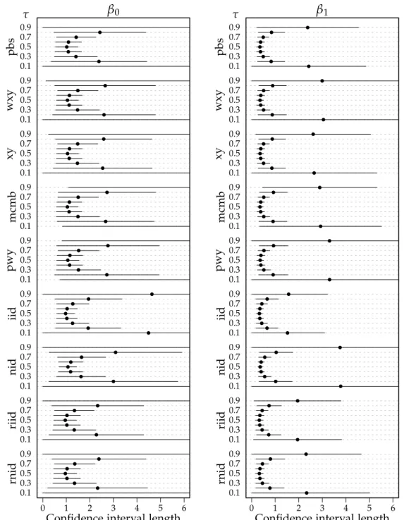
0.1 0.3 0.5 0.7 0.9 0.1 0.3 0.5 0.7 0.9 0.1 0.3 0.5 0.7 0.9 0.1 0.3 0.5 0.7 0.9 0.1 0.3 0.5 0.7 0.9 0.1 0.3 0.5 0.7 0.9 0.1 0.3 0.5 0.7 0.9 0.1 0.3 0.5 0.7 0.9 0.1 0.3 0.5 0.7 0.9 pbs wxy xy mcmb pwy iid nid riid rnid 0 1 2 3 4 5 6 β0

Confidence interval length τ 0.1 0.3 0.5 0.7 0.9 0.1 0.3 0.5 0.7 0.9 0.1 0.3 0.5 0.7 0.9 0.1 0.3 0.5 0.7 0.9 0.1 0.3 0.5 0.7 0.9 0.1 0.3 0.5 0.7 0.9 0.1 0.3 0.5 0.7 0.9 0.1 0.3 0.5 0.7 0.9 0.1 0.3 0.5 0.7 0.9 pbs wxy xy mcmb pwy iid nid riid rnid 0 1 2 3 4 5 6 β1

Confidence interval length τ

Figure 1.3: Average confidence interval lengths for the modelYi = β0+β1xi+ui,

where xi ∼ U(0, 5), β0 = β1 = 10 and ui ∼ t1. The sample size is n = 150, the number of resamples in each of the bootstrap methods is B = 1000, the number of Monte Carlo simulations is N = 1000. The circles represent the mean length, the horizontal lines are a guide to the variability of the mean length estimate and represent a naive 95% confidence interval constructed as the mean length±two times theSD of the lengths.

the true coverage probabilities for the intercept and slope parameters. As the sample size increases, most methods perform well for central τ values

but, for the intercept, their coverage probabilities fall below the nominal level at moderate and extremeτ while, for the slope, they remain relatively

unaffected. Across all sample sizes considered, the pbs and rank inversion methods give good coverage probabilities for the slope parameter.

We conjecture that this behaviour is related to the inherent difficulty as-sociated with estimating quantiles of heavy tailed distributions. Indeed the intercept in a quantile regression model actually estimatesβ0+Fu−1(τ). The

average lengths are typically twice as long for the intercept than the slope coefficient over all τ for ν ∈ {1, 2, 3, 4, 5}. However, the variability of the

lengths decreases as ngrows. This would suggest that the confidence inter-vals are tightening asnincreases but the point estimates are not converging to the true parameter values as quickly, leading to poor coverage. While not shown in the figures, as the degrees of freedom increase this phenomenon becomes somewhat more moderate and as ν → ∞, i.e. for Gaussian errors,

the ‘V’ behaviour is no longer present and all methods perform well, with the exception of the iid method.

More generally with regard to the average lengths, all methods considered experience difficulty constructing concise confidence interval lengths atτ ∈ {0.1, 0.9}. Figure 1.3 demonstrates this point for a set of fixed uniform co-variates with t1 distributed errors and n = 150. At more moderate τ, the

variability of the average lengths decreases for all models. As would be ex-pected, the average lengths and their associated variability decrease as the sample size increases and asτ becomes more moderate. Interestingly in

Fig-ure 1.3 most models are performing very similarly in terms of estimated lengths and their variability. The iid method appears to be doing quite well in terms of length, however the empirical coverage probabilities are well below the nominal level.

1.3.2 Skewed covariates

The next class of models considered take the same form as equation (1.4) with ui ∼ N(0, 1) and the covariates are sampled from a highly skewed

distribution. We considered xi ∼ χ21, χ22 and log normal with mean 0 and variance 1 on the log scale. Skewed covariates may cause issues for quantile regression estimates particularly with low sample sizes at extreme τ. The

the stability of the extreme quantile estimates. Therefore, a priori, we would assume that confidence intervals for both β0 and β1 will be affected quite significantly in the case of smalln.

Figure 1.4 is indicative of the coverage patterns exhibited by the various techniques in the presence of skewed covariates for n = 50. In this par-ticular example, we have covariates sampled from the χ2₁ distribution. The

resampling methods, with the exception of the mcmb and pwy approach, all perform quite well in terms of estimated coverages for both the slope and the intercept, they continue to work well asnincreases. The mcmb and pwy approaches exhibit a strong ‘V’ shape which is only tempered at n = 200 and for the extremely heavy tailed log normal distribution. Even atn=200, the mcmb and pwy methods continue to result in empirical coverage prob-abilities higher than the nominal level for allτ ∈ {0.1, 0.2 . . . , 0.9}.

As expected, when it comes to estimating the slope coefficient, the iid and nid methods that rely heavily on standard asymptotic normality theory perform sub-optimally across the whole range of τ considered even at n =

200. Indeed, the iid method yields empirical coverage probabilities lower than the nominal level even for the intercept parameter.

The rank inversion methods perform well over all sample sizes and τ,

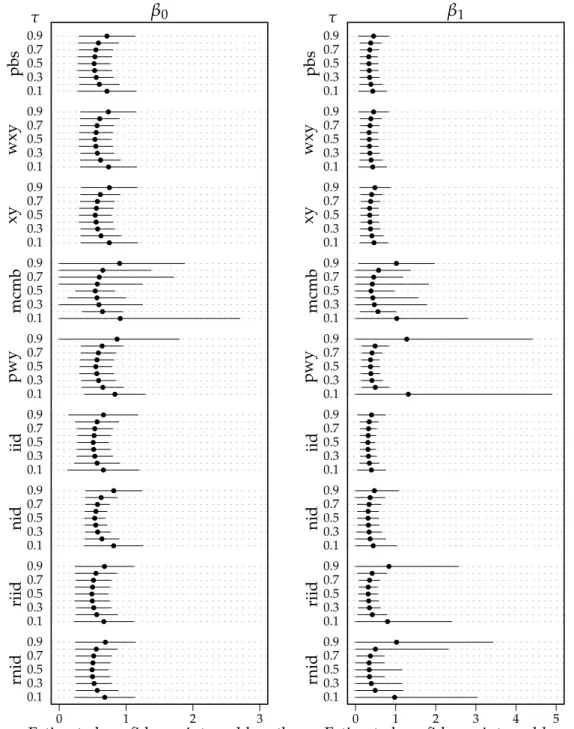
however they tend to yield empirical coverage probabilities below the nom-inal level. Figure 1.5 plots the lengths of the estimated confidence intervals for n = 100. The key feature here is the variability inherent in the mcmb and to a lesser extent, pwy, riid and rnid methods. It is generally preferable for confidence intervals to err on the side of conservatism which is why, in the case of skewed covariates, the pbs, xy and wxy methods appear to be the best performers in terms of estimated coverage and are all equally well behaved in terms of confidence interval length.

1.3.3 Multiple regression and heteroskedasticity

Here we consider a more general functional form with two covariates and allow for the possibility of heteroskedasticity,

Yi = β0+β1xi1+β2xi2+ (1+αxi1)ui. (1.5)

Models where x1 and x2 are independent are considered as well as models where x1 and x2 are bivariate Gaussian with variance 1 and various values for the correlation between x1 and x2.

Firstly, considering models with no heteroskedasticity, i.e. α = 0 but

0.1 0.3 0.5 0.7 0.9 0.1 0.3 0.5 0.7 0.9 0.1 0.3 0.5 0.7 0.9 0.1 0.3 0.5 0.7 0.9 0.1 0.3 0.5 0.7 0.9 0.1 0.3 0.5 0.7 0.9 0.1 0.3 0.5 0.7 0.9 0.1 0.3 0.5 0.7 0.9 0.1 0.3 0.5 0.7 0.9 pbs wxy xy mcmb pwy iid nid riid rnid 0.7 0.8 0.9 1.0 β0

Empirical coverage probabilities τ 0.1 0.3 0.5 0.7 0.9 0.1 0.3 0.5 0.7 0.9 0.1 0.3 0.5 0.7 0.9 0.1 0.3 0.5 0.7 0.9 0.1 0.3 0.5 0.7 0.9 0.1 0.3 0.5 0.7 0.9 0.1 0.3 0.5 0.7 0.9 0.1 0.3 0.5 0.7 0.9 0.1 0.3 0.5 0.7 0.9 pbs wxy xy mcmb pwy iid nid riid rnid 0.7 0.8 0.9 1.0 β1

Empirical coverage probabilities τ

Figure 1.4: Empirical coverage probabilities for the model Yi = β0+β1xi +ui,

where xi ∼ χ2₁, ui ∼ N(0, 1) and β0 = β1 = 10. The sample size is n = 50, the number of resamples in each of the bootstrap methods is B = 1000, the number of Monte Carlo simulations is N = 1000. The nominal coverage is 0.9.

0.1 0.3 0.5 0.7 0.9 0.1 0.3 0.5 0.7 0.9 0.1 0.3 0.5 0.7 0.9 0.1 0.3 0.5 0.7 0.9 0.1 0.3 0.5 0.7 0.9 0.1 0.3 0.5 0.7 0.9 0.1 0.3 0.5 0.7 0.9 0.1 0.3 0.5 0.7 0.9 0.1 0.3 0.5 0.7 0.9 pbs wxy xy mcmb pwy iid nid riid rnid 0 1 2 3 β0

Estimated confidence interval length τ 0.1 0.3 0.5 0.7 0.9 0.1 0.3 0.5 0.7 0.9 0.1 0.3 0.5 0.7 0.9 0.1 0.3 0.5 0.7 0.9 0.1 0.3 0.5 0.7 0.9 0.1 0.3 0.5 0.7 0.9 0.1 0.3 0.5 0.7 0.9 0.1 0.3 0.5 0.7 0.9 0.1 0.3 0.5 0.7 0.9 pbs wxy xy mcmb pwy iid nid riid rnid 0 1 2 3 4 5 β1

Estimated confidence interval length τ

Figure 1.5: Average confidence interval lengths for the modelYi = β0+β1xi+ui,

where xi ∼ χ2₁, ui ∼ N(0, 1) and β0 = β1 = 10. The sample size is n = 100, the number of resamples in each of the bootstrap methods is B = 1000, the number of Monte Carlo simulations is N = 1000. The circles represent the mean length, the horizontal lines are a guide to the variability of the mean length estimate and represent a naive 95% confidence interval constructed as the mean length±two times theSD of the lengths.

of the techniques, with the exception of the iid method, perform well even when x1 and x2 have correlation as high as 0.9.

However, when we introduce heteroskedasticity, even in a simple linear regression type scenario, i.e. β2 = 0, the results are quite different. As ex-pected, the methods that rely on the independently distributed error as-sumption, iid, riid and mcmb, do very poorly in terms of coverage for both the intercept and the slope coefficient. It is interesting that also at α = 0.5,

the methods designed to be robust to the independent error assumption begin to falter at high and low quantiles. The resampling techniques, pbs, wxy and xy, perform reasonably well for τ ∈ {0.3, 0.4, 0.5, 0.6, 0.7} over all

n. When the error is highly correlated with the covariate, e.g. α > 0.5,

ex-treme caution needs to be exercised when conducting inference on the slope parameter away fromτ =0.5.

In the multivariate case, these results still hold. Figure 1.6 demonstrates both of the above points with a sample size of n = 200. Here we have

α = 0.5, and the failure of the methods relying on the iid assumption is

evident – further, even the models designed to be robust to this assumption perform poorly for τ ∈ {0.1, 0.9}. The resampling techniques (with the

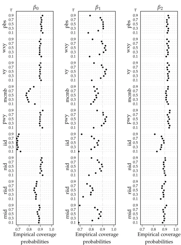
ex-ception of the mcmb method which requires the errors to be independent) deserve special mention. Looking at the slope coefficient of the variable that is not directly related to the error term, the resampling methods (with the exception of the mcmb method which requires the errors to be independ-ent) are quite consistent in their slight over estimation of the true coverage whilst the nid and rank inversion methods all perform quite well. Looking at all three coefficients jointly over the range ofτ, it is difficult to ignore the

performance of the percentile bootstrap. In terms of lengths, all methods perform quite similarly, however, the rank inversion methods exhibit more variability in their estimates than the resampling techniques.

Introducing higher correlation between the covariates, does not notice-ably affect the empirical coverage probabilities, though the lengths of the confidence intervals tend to increase. The major insight is that in the pres-ence of high correlation between the covariates, the coverage will be largely unaffected, though it is likely that the length of the confidence interval will be greater than in the uncorrelated case.

0.1 0.3 0.5 0.7 0.9 0.1 0.3 0.5 0.7 0.9 0.1 0.3 0.5 0.7 0.9 0.1 0.3 0.5 0.7 0.9 0.1 0.3 0.5 0.7 0.9 0.1 0.3 0.5 0.7 0.9 0.1 0.3 0.5 0.7 0.9 0.1 0.3 0.5 0.7 0.9 0.1 0.3 0.5 0.7 0.9 pbs wxy xy mcmb pwy iid nid riid rnid 0.7 0.8 0.9 1.0 β0 Empirical coverage probabilities τ 0.1 0.3 0.5 0.7 0.9 0.1 0.3 0.5 0.7 0.9 0.1 0.3 0.5 0.7 0.9 0.1 0.3 0.5 0.7 0.9 0.1 0.3 0.5 0.7 0.9 0.1 0.3 0.5 0.7 0.9 0.1 0.3 0.5 0.7 0.9 0.1 0.3 0.5 0.7 0.9 0.1 0.3 0.5 0.7 0.9 pbs wxy xy mcmb pwy iid nid riid rnid 0.7 0.8 0.9 1.0 β1 Empirical coverage probabilities τ 0.1 0.3 0.5 0.7 0.9 0.1 0.3 0.5 0.7 0.9 0.1 0.3 0.5 0.7 0.9 0.1 0.3 0.5 0.7 0.9 0.1 0.3 0.5 0.7 0.9 0.1 0.3 0.5 0.7 0.9 0.1 0.3 0.5 0.7 0.9 0.1 0.3 0.5 0.7 0.9 0.1 0.3 0.5 0.7 0.9 pbs wxy xy mcmb pwy iid nid riid rnid 0.7 0.8 0.9 1.0 β2 Empirical coverage probabilities τ

Figure 1.6: Empirical coverage probabilities for the model defined by equation (1.5), where x1 and x2 are multivariate Gaussian, both with variance 1 and correlation coefficient 0.5;ui ∼ N(0, 1);α=0.5 and β0 = β₁ = β2 =10. The sample size is n = 200, the number of resamples in each of the bootstrap methods isB=1000, the number of Monte Carlo simulations isN=1000. The nominal coverage is 0.9.

1.4 c o n c l u s i o n

The aim of this chapter was to revisit and extend the analysis performed by Kocherginsky, He and Mu (2005), incorporating additional techniques and evaluating their effectiveness for sample sizes n ≤ 200 and over a broad range of conditional quantiles. We considered simple models with only a few parameters so as to isolate the effect of the various pathologies. This is an important distinction to make as some of the methods considered were designed primarily for use in large samples. For example the mcmb method is most valuable when estimating high dimensional models.

The percentile bootstrap was found to be a sound performer exhibiting significant robustness to heteroskedasticity, heavy tailed error distributions and skewed covariates. In most cases it was found to be better than, or at least on par with, more complex resampling techniques as well as the nid and rank inversion methods in terms of coverage probabilities, average lengths and the variability of those lengths. The performance of the per-centile bootstrap was somewhat surprising given its simplicity relative to the other resampling techniques. However, Hahn (1995) foreshadowed this result, showing the asymptotic empirical coverage probability of the boot-strap percentile method to be equal to the nominal coverage probability even when the error term is not independent of the regressor. It is noted in the R documentation for the quantreg (Koenker, 2013) package that the percentile method is a “refinement that is still unimplemented”, though it is not difficult to code directly.

All methods did not perform well when estimating the intercept for high and low quantiles in the presence of heavy tailed errors. Also, when there is strong heteroskedasticity caused by one variable, the estimated coverage probabilities for the corresponding coefficient can be severely underestim-ated at high and low quantiles. When the error term is dependent on one or more covariates and extremeτ is of interest, caution should be used when

constructing confidence intervals, even for largen.

The nid method generally performed quite well, except in the presence of heavy tailed covariates. This was also noted in Kocherginsky, He and Mu (2005) where they similarly found the nid method tended to underestimate the coverage. The reason being that when a covariate is too heavy tailed, the asymptotic normality of ˆβτ would fail. In this case, the percentile boot-strap or rnid would be suggested, noting that the percentile bootboot-strap gives consistently tighter lengths than the rnid approach.

The mcmb approach uses the MCMB-A algorithm which is not robust in the presence of heteroskedasticity. At high and lowτeven in iid models, the

mcmb approach did quite poorly and as such would not be recommended in all but the most well behaved of models whenn ≤200.

As expected the iid and riid methods did not perform well when the iid assumption was violated and did not outperform the more robust methods in the standard iid error models. Thexy-pair bootstrap and pwy techniques performed well, except when there were correlated covariates.

The rank test inversion methods, riid and rnid, occasionally generated confidence intervals of infinite length, particularly with small sample sizes, heavy tailed covariates and extreme τ. If this is observed in practice, the

percentile or paired bootstrap or nid method would be an appropriate al-ternative.

The confidence interval lengths for the rank inversion methods were often observed to be far more variable than the other methods. This has much to do with the relatively small sample sizes and the way the confidence inter-vals are generated by inverting a test statistic. With less data points, particu-larly at extremeτ, the inversion process has to search further afield to find

appropriate upper and lower bounds. In the other methods, a standard er-ror is estimated and a standard symmetric confidence interval is calculated. The xy-pair bootstrap and the nid method on average gave the smallest confidence intervals whilst maintaining acceptable coverage performance.

To summarise, the percentile bootstrap approach is a simple, intuitive and viable alternative for constructing confidence interval estimates in the quantile regression setting. Hahn (1995) showed that the percentile boot-strap provides asymptotically correct coverage probabilities and we found its small sample performance to be impressive.

2

S C A L E E S T I M AT I O N

2.1 i n t r o d u c t i o n

A reliable estimate of the scale of a data set is a fundamental issue in stat-istics. For example the scale of the residuals from a regression model is often of interest, whether it be parametrically estimating confidence inter-vals, determining a goodness of fit measure, performing model selection, or identifying unusual observations. The robustness of quantile regression parameter estimates, described in Chapter 1, to y-outliers does not extend to the error distribution – extreme observations in the y space yield outly-ing residuals which can interfere with subsequent analyses. This led us to consider the problem of finding reliable robust estimates of scale.

While scale parameters are sometimes treated as nuisance parameters, a talk given by Raymond Carroll at the University of Technology, Sydney, in June 2013 shared the same title as his 2003 paper, “Variances are not always nuisance parameters” indicating that finding reliable estimates of scale is just as important a problem in 2013 as it was in 2003.

Robust estimates of scale are important for a range of applications, from true scale problems, to outlier identification, and as auxiliary parameters for more involved analyses. Recent work concerning robust scale estimation includes Boente, Ruiz and Zamar (2010), Wu and Zuo (2008) and Van Aelst, Willems and Zamar (2013).

There are two aims in formulating a robust estimator: the first is to reduce the potential bias caused by outliers and the second is to maintain efficiency when there are no outliers present. These two aims are generally in conflict with one another. In the scale setting, the median absolute deviation from the median (MAD) is commonly used in practice, despite its poor Gaussian efficiency. The estimator Qn (Rousseeuw and Croux, 1993) is a significant

improvement on the MAD in terms of efficiency whilst maintaining a high level of robustness. This chapter presents an alternative robust scale estim-ator which trades some robustness for desirable efficiency properties.

We propose a new robust scale estimator, the pairwise mean scale es-timator Pn, which combines familiar features from a number of commonly

used robust estimators and possesses surprising efficiency properties (Tarr, Müller and Weber, 2012). In contrast to Qn, which utilises pairwise

differ-ences, Pn is based on pairwise means. The most basic form of Pn is

calcu-lated as the IQR of the pairwise means, yielding a scale estimator that can

be viewed as a natural complement to the Hodges-Lehmann location estim-ator (Hodges and Lehmann, 1963). A generalisation, Pn(τ), considers the

distance between the(1±τ)/2 quantiles of the empirical distribution of the

pairwise means. Unless otherwise specified, the notation Pn is equivalent to

Pn(0.5). Extensions are investigated that are based around Winsorising and

trimming. We also implement a form of adaptive trimming which is shown to achieve the maximal breakdown value of 50%.

Our investigation into the efficiency properties of the pairwise mean scale estimator is based on Randal (2008) who calculates efficiencies of estimators relative to the corresponding maximum likelihood estimators at a particu-lar distribution. This method facilitates easier comparison than the method used in the seminal study by Lax (1985).

The pairwise mean scale estimator fits into the family of generalised L -statistics (GL-statistics) which encompasses broad classes of statistics of in-terest in nonparametric estimation; in particular,L-statistics,U-statistics and U-quantile statistics (Serfling, 1984). Thus, a wide range of statistics related to scale estimation are embedded into a single unified class. For example, the IQR; variance; trimmed and Winsorised variance; and Qn all fit within

the class of GL-statistics.

M-estimators are an important exception to the class ofGL-statistics. The

MAD is the most prominent robust scale estimator that sits under the M -estimator umbrella. An advantage ofPn over M-estimators of scale is that it

does not require a location estimate.

The next section outlines an important family of statistics and introduces some common decomposition techniques used throughout the thesis to de-rive limiting distributions. A review of some existing scale estimators and their properties are given in Section 2.3. Section 2.4 formally defines the estimator Pn along with possible generalisations and its breakdown value

is found. The influence function and asymptotic normality of Pn are also

derived in Section 2.4. In addition to being an intuitive estimate of scale, one of the primary advantages ofPn is its high efficiency over a broad range

of distributions. The results of a simulation study are given in Section 2.5 which show how Pn compares favourably with other robust estimates of

2.2 b a c k g r o u n d t h e o r y

This section outlines some theory that will be used throughout the thesis. We begin by introducing U-statistics and U-quantile statistics. The Hoeffd-ing decomposition, a classical approach to workHoeffd-ing with U-statistics, and Hermite polynomials, a classical approach to decomposing Gaussian pro-cesses, are both briefly discussed. These techniques will be most relevant in Chapter 3. Finally, a broader class of statistics that encompasses bothU -andU-quantile statistics is introduced.

2.2.1 U- and U-quantile statistics

Let X1, . . . ,Xn be a set of iid observations and g be a symmetric bivariate

kernel,g :R27→ R. Hoeffding (1948) defines aU-statistic (of order 2) as, 2

n(n−1)

∑

An example of aU-statistic is the sample variance which is aU-statistic with g(x,y) = (x−y)2/2.

A U-quantile statistic is a quantile of the distribution function of the ker-nels of theU-statistic. LetG(t) =P(g(X1,X2)≤t)be theCDFof the kernels with corresponding empirical distribution function,

Gn(t) = 2

n(n−1)

∑

for some interval I ⊆R. Note that (2.1) is aU-statistic with kernel,

h(x,y;t) =I{g(x,y) ≤t}, ∀ x,y ∈ R and t ∈ I. (2.2) For p ∈ (0, 1), the corresponding sampleU-quantile is,

G_n−1(p) =inf{t: Gn(t)≥ p}.

2.2.1.1 Hoeffding decomposition

The Hoeffding decomposition is the classical mode of attack for analysing the asymptotics of non-degenerateU-statistics. Leth1(x;t) =E[h(x,X1;t)]−

G(t). For all t∈ I, write the difference, Gn(t)−G(t) = 1 n(n−1)_i6

∑

as, Gn(t)−G(t) =Wn(t) +Rn(t), where, Wn(t) = 2 n n

∑

∑

The function h1(x;t) is defined for allx ∈ Rand t ∈ I and if X1, . . . ,Xn are

independent standard Gaussian, h1(x;t) =

Z

h(x,y;t)φ(y)dy−G(t),

and hence,E[h1(X2;t)] =0.

2.2.1.2 Hermite decomposition

As Beran (1994) notes, the classical approach based on the Hoeffding decom-position is not always appropriate for establishing the asymptotic behaviour of U-statistics when working with long range dependent (LRD) sequences, as considered in Chapter 3. An alternative approach is to use a decomposi-tion based on Hermite polynomials. Thekth Hermite polynomial, Hk(x), is

defined as, Hk(x) = (−1)kex 2_/2 " dk dxke −x2_/2 # .

Using this definition, the first four Hermite polynomials are: H0(x) = 1, H1(x) =x, H2(x) = x2−1 and H3(x) = x3−3x.

Hermite polynomials build an orthogonal basis. To see this let Z be a standard Gaussian random variable then,

E[Hk(Z)Hk(Z)] =k!,

and for allk 6= j,

E[Hk(Z)Hj(Z)] =0.

Furthermore, let J be the set of functions J such that E[J(Z)] = 0 and

E[J2(Z)]<∞ then every function J ∈ J can be written as

J(Z) = ∞

∑

with Hermite coefficientsαk =E[J(Z)Hk(Z)]. TheHermite rankof a function

J is defined as m=inf{k ≥1 :αk 6=0}. We therefore have,

J(Z) = ∞

∑

Let X and Y be independent standard Gaussian random variables. The kernel function defined in (2.2) can be expanded in a bivariate Hermite polynomial basis as follows,

h(X,Y;t) = I{g(X,Y)≤t}=

∑

αp,q(t)

p!q! Hp(X)Hq(Y), (2.5) for t ∈ I, where, αp,q(t) = Eh(X,Y;t)Hp(X)Hq(Y). The constant term in

the bivariate Hermite decomposition (2.5) is given byα0,0(t),

α0,0(t) = G(t) =

Z Z

h(x,y;t)φ(x)φ(y)dxdy for all t ∈ I.

As we will see in Chapter 3, the Hermite rank of the class of functions

{h(·,·;t)−G(t),t ∈ I} plays a crucial role in understanding the asymptotic behaviour of empirical quantiles of the U-process Gn. Analogously to the

univariate case, the Hermite rank of the bivariate functionh(·,·;t)is defined as the smallest positive integerm(t)such that there exist pand q satisfying p+q =m(t) and αp,q(t) 6=0. Thus we can write (2.5) as,

h(X,Y;t)−G(t) =

∑

p+q≥m(t)

αp,q(t)

p!q! Hp(X)Hq(Y).

Further details on Hermite polynomials and their properties can be found, among others, in Beran (1994), Giraitis, Koul and Surgailis (2012) and Beran et al. (2013).

2.2.2 Generalised L-statistics

Serfling (1984) introduces an extension of U-quantile statistics known as generalisedL-statistics (GL-statistics). Many robust scale estimators are nes-ted within the class of GL-statistics, including our new scale estimator Pn.

Again restricting attention to symmetric bivariate kernels, g(x1,x2), the GL-functional is defined as,

T(G) = Z 1 0 w (p)G−1(p)dp+ d

∑

wherewis a function for the smooth weighting ofG−1(p)andajare discrete

coefficients for G−1(pj) (Serfling, 1984). Evaluation of the GL-functional at

the corresponding sample distribution of g(X1,X2), yields the following representation ofGL-statistic, Tn =T(Gn) = Z 1 0 w(p)G −1 n (p)dp+ d

∑

The class of generalisedL-statistics (GL-statistics) encompassesL-statistics, U-statistics and U-quantile statistics and as such covers a range of scale es-timates. Janssen, Serfling and Veraverbeke (1984) and Serfling (1984) study the asymptotic properties of GL-statistics in some detail.

2.3 r e v i e w o f r o b u s t s c a l e e s t i m at i o n t h e o r y

We define any estimator, Sn, that is shift invariant and scale equivariant to

be a scale estimator. That is, for a set ofnobservations, x, and any constant c ∈R, Sn(x+c) =Sn(x) and Sn(cx) =|c|Sn(x).

A traditional way to measure the spread of a data setxis the (non-robust) sample standard deviation,

SD(x) = s 1 n−1 n

∑

where ¯x = n−1∑_in=1xi is the sample mean. However, it is well known that

theSDis not robust to outlying observations. This section outlines some key features of robust estimators and defines some common robust alternatives to theSD, many of which fit within the class of GL-statistics.

2.3.1 Measures of robustness

The core of this thesis focusses on robust estimation techniques. An intro-duction to the philosophy underlying robust procedures is found in Mor-genthaler (2007). In general, an estimator is said to be robust if it is relatively unaffected by arbitrary corruption to some small proportion of observations. The proportion of corrupted observations in the data set will be referred to asε. Themost robustestimators return bounded estimates asε↑ 0.5, i.e. up to

half of the data set may experience arbitrary corruption. In practice, it is not likely that univariate samples will have such a high level of contamination so we do not restrict attention solely to the most robust methods.

Two popular ways of describing the robustness properties of estimators are the breakdown value and the influence function.

2.3.1.1 Breakdown value

The breakdown value of an estimator,ε∗, is the smallest value ofεfor which

the estimator, Tn, when applied to the ε-corrupted sample ex, can be forced to the boundary of the parameter space.

Hodges (1967) and Hampel (1971) were the first to propose and define the concept of a breakdown value. Hubert and Debruyne (2009) provide a recent overview of its history. The classical definition of the asymptotic contamination breakdown value of a location estimatorTn atx is

ε∗(x,Tn) =inf{ε|b(ε;x,Tn) =∞},

whereb is the maximum bias that can be caused byε-corruption:

b(ε;x,Tn) = sup|Tn(ex)−Tn(x)|,

and the supremum is taken over the set of allε-corrupted samplesxe.

For a scale estimator,Sn, we need to adjust the classical definition slightly,

to include the possibility of implosion, i.e. returning a value of zero. In finite samples this is defined by,

ε∗(x,Sn) =max ( m n : sup e x Sn(xe) <∞ and inf e x Sn(xe) >0 ) ,

wherem is the number of observations in x replaced with arbitrary values (Huber, 1981, p. 110).

2.3.1.2 Influence function

Hampel (1974) defines the influence function for a functionalT at the distri-bution Fas,

IF(x;T,F) = lim e↓0

T((1−e)F+eδx)−T(F)

e , (2.8)

where the distribution δx has all its mass at x. The influence function is

es-sentially the first order Gâteaux derivative of a functionalTat a distribution F in the direction of δx. It represents the effect of a point mass

contamina-tion at x on the estimate, in a sense, capturing the asymptotic bias caused by the contamination.