F
EDERAL
R
ESERVE
B
ANK OF
P
HILADELPHIA
Ten Independence Mall, Philadelphia, PA 19106-1574• (215) 574-6428• www.phil.frb.org
W
ORKING
P
APERS
R
ESEARCH
D
EPARTMENT
WORKING PAPER NO. 01-6/R
EXPLAINING THE DRAMATIC CHANGES IN PERFORMANCE
OF U.S. BANKS: TECHNOLOGICAL CHANGE,
DEREGULATION, AND DYNAMIC CHANGES IN
COMPETITION
Allen N. Berger
Board of Governors of the Federal Reserve System
The Wharton Financial Institutions Center, University of Pennsylvania
Loretta J. Mester
Federal Reserve Bank of Philadelphia
The Wharton School, University of Pennsylvania
Explaining the Dramatic Changes in Performance of U.S. Banks: Technological Change, Deregulation, and Dynamic Changes in Competition*,†,‡
Allen N. Berger
Board of Governors of the Federal Reserve System
The Wharton Financial Institutions Center, University of Pennsylvania Loretta J. Mester
Federal Reserve Bank of Philadelphia
Finance Department, The Wharton School, University of Pennsylvania August 2002
Published in the Journal of Financial Intermediation, 12 (2003), pp. 57-95
The views expressed in this paper do not necessarily represent those of the Federal Reserve Bank of
*
Philadelphia, the Board of Governors of the Federal Reserve System, or the Federal Reserve System.
We thank the editor Anjan Thakor and the anonymous referees for very helpful suggestions for improving
†
the paper. We also thank Dennis Fixler, Diana Hancock, Dave Humphrey, Rick Lang, Mike Mohr, Leonard Nakamura, Jack Triplett, Greg Udell, Bob Yuskavage, Kim Zieschang; and participants at the Brookings Workshop on Measuring Banking Output, Washington, DC; the Conference on Service Sector Productivity and the Productivity Paradox, Ottawa, Canada; the Financial Management Association meetings; the Australian Industry Economic Conference, Canberra; and the Georgia Productivity Workshop, Athens, GA, for helpful comments and advice; Seth Bonime, Chris Malloy, Nate Miller, and Avi Peled for excellent research assistance; and Sally Burke for expert editorial assistance.
Correspondence to Berger at Mail Stop 153, Federal Reserve Board, 20th and C Sts. N.W., Washington,
‡
D.C. 20551; phone: (202) 452-2903; fax: (202) 452-5295; email: [email protected]. To Mester at Research Department, Federal Reserve Bank of Philadelphia, Ten Independence Mall, Philadelphia, PA 19106-1574; phone: (215) 574-3807; fax: (215) 574-4303; email: [email protected].
Technological Change, Deregulation, and Dynamic Changes in Competition*,†,‡
Abstract
We investigate the effects of technological change, deregulation, and dynamic changes in competition on the performance of U.S. banks. Our most striking result is that during 1991-1997, cost productivity worsened while profit productivity improved substantially, particularly for banks engaging in mergers. The data are consistent with the hypothesis that banks tried to maximize profits by raising revenues as well as reducing costs. Banks appeared to provide additional or higher quality services that raised costs but also raised revenues by more than the cost increases. The results suggest that methods that exclude revenues when assessing performance may be misleading.
JEL Classification Numbers: G21, G28, E58, E61, F33
Technological Change, Deregulation, and Dynamic Changes in Competition 1. Introduction
Much of the attention regarding the recent boom in the U.S. economy has centered on improvements in productivity associated with technological progress in information processing, telecommunications, and other technologies. Performance gains in the financial industry have also been linked to improvements in financial technologies, including new tools of financial engineering, and the more advanced use of statistical techniques. This raises the obvious question: how have these developments affected the performance of banks?
To address this broad question, we begin by noting that the banking industry may have benefitted considerably from advances in both nonfinancial and financial technologies. On the one hand, due to consolidation and deregulation, banking has become more competitive, and one would expect that many inefficiencies have been rooted out. Banks have used information processing to process deposit and loan customer information and to evaluate risks more efficiently, and telecommunications technologies to transmit this information and to process payments more quickly with fewer resources. This might suggest an improvement in cost productivity during the 1990s. On the other hand, banks have also adopted new financial technologies and new services, and improved the quality of some of the existing services. These additional services or higher service quality may have raised costs. So it may not be obvious how measured cost productivity has been affected. Similarly, it is difficult to judge a priori how profit productivity—which incorporates revenues as well as costs—would be affected, since this depends in part on how much more bank customers have been willing to pay for the innovations introduced by banks.
Our purpose in this paper is to examine empirically the two questions suggested by the above discussion. First, during the 1990s, has the cost productivity of the U.S. banking industry improved or worsened? Second, during the same time period, has the profit productivity of the U.S. banking industry improved or worsened?
A striking finding of this study is that during the recent 1991-1997 period, cost productivity significantly
worsened. The predicted cost of producing a given level of output actually increased, controlling for business conditions in the local market (which include market interest rates). Another striking result in our study is that profit productivity improved dramatically over the same 1991-1997 period. Our findings are consistent with the hypothesis that banks provided additional services or higher service quality, which may have raised costs but also raised revenues by more than the cost increases.
in conventional market power in setting output prices, perhaps associated with greater market concentration after consolidation of the industry. However, some evidence presented below suggests that this is not likely the case—local market concentration changed little on average over time, and the changes that did occur are associated with price changes that contribute very little to profitability increases. A more likely explanation is that the higher profitability indicates an ongoing process of innovation. Early adopters of an effective new technology temporarily
earn higher profits, but the abnormal returns are competed away as the technology is diffused throughout the industry. When another promising new technology comes along, the process starts again. An industry like banking that has adopted a number of successful new technologies at different points in time can have supernormal profits on average for a considerable period, although different firms may be innovating and earning the extra profits at different points in time.
Our analysis of changes in banking industry performance uses some of the recently developed concepts and techniques from the cross-section efficiency literature. The three main sources of the changes in costs and profits over time investigated are: (1) changes in managerial best practice in the industry, which includes technological change and the extent to which the best-practice firms adopt it, (2) changes in cross-section inefficiency or dispersion from this best-practice technology, and (3) changes in “business conditions,” or economic factors exogenous to the banks. These first two components—changes in best practice and changes in inefficiency—together form the more traditional notion of change in productivity.
We analyze the sources of change in performance over the period 1984-1997 using three different optimization concepts—cost minimization, standard profit maximization, and alternative profit maximization. These concepts are based on economic optimization in reaction to market prices and competition, rather than solely on the use of technology, as are some government and research measures of productivity change. To our knowledge, only one research study has measured alternative profit performance/productivity change, no prior study has measured standard profit change, and no prior study of changes in performance or productivity has applied more than one of these concepts. We use all three concepts to ensure a comprehensive look at the data.
We decompose productivity change into the changes in the industry’s best practice versus changes in inefficiency. The estimated best practice reflects the behavior of the best existing banks, but not any “true” efficient point, which would reflect the available technology and optimal responses to market prices and other business conditions. Changes in both managerial best practice and industry efficiency may be driven by technological progress, regulatory innovation, or other changes in competitive conditions. Thus, even if we rule out technological
regress, productivity may worsen over time because of changes in regulation or competitive conditions. Past studies often found negative productivity growth for U.S. banks, and as indicated above, we find negative cost productivity change during the 1990s.
Section 2 gives background information on performance trends in U.S. banking. Section 3 reviews prior analysis of bank productivity change from both government statistics and research studies. Section 4 lays out the optimization concepts and how they are applied to decompose changes in performance. Section 5 gives the design of our empirical analysis. Section 6 displays our main empirical results, and Section 7 examines a number of alternative potential explanations of the empirical results. Section 8 draws conclusions.
2. Performance trends in U.S. banking
The mid-1980s to the early 1990s was a period of relatively poor performance of U.S. banks. Banks began to realize problems with commercial real estate loans and loans to less developed nations, leading to performance problems and a “credit crunch” in the early 1990s. From that time until the end of our sample period in 1997, the U.S. banking industry enjoyed substantially improved performance.
Some of these performance trends are illustrated in Table I. Profitability as measured by mean return on equity rose by more than three-quarters from 6.49% at the beginning of our sample in 1984 to 11.49% by 1997. An alternative measure of profitability, mean return on gross total assets or return on GTA, rose by almost 2/3 from 68.8 basis points to 113.4 basis points. The revenues/costs ratio also rose sharply, by over 3/4, from 16.3% in 1984 to1
29.4% in 1997. Nonperforming loans/total loans showed substantial improvement in the proportion of loans that were nonperforming (past due at least 90 days or on nonaccrual basis), which fell by about half, from 5.18% of loans in 1984 to 2.57% in 1997, consistent with macroeconomic improvements.
[Table I goes here]
Table I also shows that cost ratios declined dramatically over time. Mean costs/equity and costs/GTA fell by almost one-half and one-third, respectively, over the sample period. However, our estimates, discussed below, show that cost productivity, which takes into account the businesses conditions faced by the banks, actually worsened over this period. One of the reasons for this seeming contradiction is that the rates faced by banks to raise funds fell dramatically over time—e.g., the average interest rate faced on core deposits dropped by about 2/3 (from 6.82%in 1984 to 2.31% in 1997). Thus, bank cost ratios fell, but not as much as would be predicted by the changes in business conditions faced, particularly the market interest rates faced.
Based on these data and other factors, our main analysis focuses on explaining the changes in costs and profits over the subintervals 1984-1991 and 1991-1997, as well as over the entire 1984-1997 interval. For robustness, we also segment the data into other subintervals, examine small and large banks separately, analyze whether mergers explain the results, and assess the performance effects of industry entry and exit.
The last three columns in Table I investigate two trends that could potentially help explain part of the improvement in profit performance over time. The standard deviations of return on equity (ROE) and of return on assets (ROA) over the past three, four, or five years (the longest for which annual return data on the bank is available) are proxies for bank risk. The local deposit market Herfindahl index of concentration (HERF) is a measure of the potential for the exploitation of conventional market power. We investigate below two alternative explanations of the improvement in bank performance—an increase in risk-taking and an increase in conventional market power. The raw data shown here do not provide much support for these explanations—the standard deviations of the earnings ratios appear to have decreased over time, and the increase in local market concentration over time is quite small.
Finally, the first column of Table I shows that the industry has been consolidating rapidly, with the number of banks declining by more than 1/3 in 13 years, mostly through merger activity. Results below suggest that mergers may have played an important role in the dramatic changes in bank performance—merging banks appear to have increased costs per unit of output but made up for this by raising revenues even more.
3. Prior analysis of bank performance change 3.1 Government productivity measures
Government agencies typically measure productivity by the ratio of an output index to an input index. The U.S. Bureau of Labor Statistics (BLS) developed a labor productivity measure for the commercial banking industry (SIC 602). They measure physical banking output using a “number-of-transactions” approach based on demand deposits (number of checks written and cleared, and number of electronic funds transfers), time deposits (weighted index of number of deposits and withdrawals on regular savings accounts, club accounts, CDs, money market accounts, and IRAs), ATM transactions, loans (indexes of new and existing real estate, consumer installment, and commercial loans, and number of bank credit card transactions), and number of trust accounts, each weighted by the proportion of employee hours used in the activity. Employee labor hours are used as the denominator of the productivity index, although the BLS also computes an output per employee measure. The BLS index for banking productivity per employee hour grew at an annualized rate of 3.09% over 1984-1997, which reflects rates of change of 2.99% and 3.20% over 1984-1991 and 1991-1997, respectively. These data indicate banking productivity rising
at a slower pace than the rest of the corporate sector.2
The Bureau of Economic Analysis (BEA) also uses labor productivity to update its output measure for banking. The BEA benchmarks the gross product originating (GPO) in banking every five years. For nonbenchmark years, real output in the banking sector is estimated by extrapolating the nominal measure of output in a benchmarking year using the rate of growth of the number of full-time equivalent employees, in effect assuming that labor productivity remains constant for five years (see Yuskavage, 1996). However, a method that estimates a decomposition of the aggregate figures has been devised, and it shows a 0.8% annual change in real output per hour over the 1989-1997 period for the Finance, Insurance, and Real Estate sector, of which banking is a part (Corrado and Slifman, 1999).
3.2 Research studies of productivity change
Several academic studies have measured productivity change. We slightly reinterpret some of their results using our own terminology. The literature often calls shifts in the best-practice frontier “technological” change, but we prefer to keep explicit the distinction between technology used by the best-practice banks and the theoretically best technology available.3
Berger and Humphrey (1992) used the thick frontier approach to compare bank cost efficiency and to study shifts in best-practice costs between 1980, 1984, and 1988 using data for virtually all U.S. banks. They found that when the shifts were not adjusted for changes in business conditions, average costs increased for all but the very largest efficient banks in the 1980-1984 interval, followed by decreases in average costs for all sizes in the 1984-1988 period. The increase in costs in the earlier period may in part reflect the deregulation of deposit rates. To the extent that the industry performed more poorly because of an increase in competitiveness that raised deposit rates, this may be a social good, because the benefits to depositors from higher rates may outweigh the higher costs to banks. When the shifts in the average cost frontiers were adjusted for changes in the business conditions, an increase in costs was still found for the 1980-1984 period, but a decrease was no longer found for the 1984-1988 period.
Bauer, Berger, and Humphrey (1993) used a panel data set of 683 banks with over $100 million in assets from states that allowed branching and that were continuously in existence during 1977-1988 to estimate total factor cost productivity growth for the best-practice banks. They found an average annual growth rate of !2.28% to 0.16%, depending on the estimation method used. The poor productivity growth was attributed to higher costs of funding because of high market rates, elimination of deposit rate ceilings, and increased competition from nonbank financial intermediaries, which increased demand for funds, reduced the supply of deposits, and increased the convenience
banks provided through more branches. The increase in deposit rates, increase in nonbank competition, and better convenience all made consumers better off, but because quality of service is difficult to account for in the estimation, the higher quality showed up as a decrease in productivity.
Humphrey (1993) used the same data set to investigate the effect on costs from shifts in the cost function. Measures were derived from a simple time trend, from a time-specific index, and from annual shifts in cross-section cost functions. All three methods yielded similar estimates, with shifts in the cost function implying cost increases averaging 0.8% to 1.4% per year, and small banks (assets of $100 million-$200 million) experiencing larger increases on average than large banks. Again, much of the decline in cost productivity was attributed to deregulation of deposit rates, which has an offsetting benefit to depositors.
Again using these data, Humphrey and Pulley (1997) estimated changes in predicted profits using the alternative profit function over the 1977-1988 period and decomposed the changes that occurred after deregulation (1984-1988) into internal bank-initiated adjustments to the new regulatory structure and external changes in banks’ business conditions. They found that for banks with assets over $500 million, the rise in profits from the 1977-1981 period to the 1981-1984 period resulted from a shift in the profit function and changes in business conditions, particularly deposit deregulation. Only business conditions accounted for the rise in large banks’ profits from 1981-1984 to 1985-1988. For smaller banks (assets of $100 million-$500 million), there was little increase in profits between 1977-1981 and 1981-1984, and in the later period, their experience was similar to that of larger banks. The same patterns held after controlling for efficiency.
Stiroh (2000) used a panel data set of 661 top-tier bank holding companies continuously in existence during 1991-1997. He used several different specifications of outputs and several different methods of measuring cost productivity change and found small cost productivity improvements of between 0.05% and 0.47% annually. One of his specifications was similar to ours in terms of the output and input definitions, but he included many fewer variables measuring business conditions in his cost function estimations than in our specification. This is a significant difference and is likely to explain much of the difference between his results and ours. While we both find that total costs rose over the 1991-1997 period, our decomposition of this cost change between that attributable to productivity change and that attributable to a change in business conditions differs. Stiroh found that cost productivity increased thereby reducing costs, but changes in business conditions contributed to higher costs. We find that cost productivity decreased thereby raising costs, but changes in business conditions put downward pressures on costs. The difference is likely because Stiroh’s business conditions include only variable outputs, fixed netputs, and input prices. In
contrast, in addition to these, we control for a number of additional business conditions in the market, including state income growth, market nonperforming loans, the extent of interstate branching, urban vs. rural market, market concentration, and federal regulator. Some of these conditions, like nonperforming loans and state income growth, were generally improving over the period and likely improved bank performance in a number of ways, including fewer costs expended dealing with problem loans. To the extent that these improved conditions are exogenous to the bank, we would not want to conclude that improved performance derived from these conditions is a productivity improvement for the bank. Rather, we would want to label this as an improvement in the exogenous business conditions faced by the bank. In contrast, Stiroh's methodology would label this as an improvement in bank productivity.
Several research efforts used linear programming methods to measure changes in productivity. These methods are nonstochastic and do not allow for random error. The productivity changes are based on quantities of outputs and inputs without regard to prices, so there is no way to determine whether banks became more or less productive in an economic sense or responded more or less appropriately to market price signals.
Devaney and Weber (2000) investigated whether the market structure of rural banking markets affected productivity growth over 1990-1993. They used linear programming to calculate the Malmquist productivity index, which decomposes productivity changes into changes in efficiency, shifts in the production function, and changes in the scale of operations. They found positive productivity growth at rural banks over 1990-1993. Shifts in the production frontier were the driving force of this productivity growth.
Wheelock and Wilson (1999) also used linear programming and decomposed the change in productivity into its change in efficiency and frontier shift components. While banks on the frontier improved over the period 1984-1993, productivity declined on average during this period because of reductions in efficiency. Most banks, particularly smaller banks (assets below $300 million), were not able to adapt quickly to changes in technology, regulations, and competitive conditions and fell further away from the efficient frontier.
Similarly, Alam (2001) applied linear programming to a balanced panel of 166 banks with greater than $500 million in assets and uninterrupted data from 1980 to 1989. She found that productivity surged between 1983 and 1984, retreated over the next year, and grew again between 1985 and 1989. The main source of the productivity growth was a shift in the frontier rather than a change in efficiency.
4. The optimization concepts and the decomposition of cost and profit changes 4.1 Cost minimization
The cost minimization concept assumes that firms minimize variable costs subject to exogenously given prices of variable inputs, quantities of variable outputs, quantities of fixed netputs (fixed inputs or outputs), environmental factors, their own managerial inefficiency, and random error. This concept is implemented using a standard cost function that relates variable costs to these exogenously given conditions. For simplicity, the inefficiency and random error are assumed to be multiplicatively separable from the rest of the cost function, and all of the variables (other than dummies) are measured in natural logs:
lnC = f (X ) + C C lnu + C ln,C. (1) The variable lnC measures log of variable costs (including both operating and interest expenses); f (C @) is the best-practice (log) cost function; X C/ (lnw, lny, lnz, lnv) is the set of logged exogenous “business conditions” that affect costs, specifically, variable input prices (lnw), variable output quantities (lny), fixed netput quantities (lnz), and environmental variables (lnv). The 4 lnu term denotes an inefficiency factor that is zero for best-practice firms and
C
raises costs for other firms. The ln,C term is a random error assumed to have zero mean each period.
We represent the cost of the industry at time t by the predicted cost of a bank with average business conditions, average inefficiency for the period, and a zero random error. This gives exp[f (X )] Ct $Ct C exp[lnu ], where$Ct X gives the average values of the business condition regressors at time t and $ ln$u gives the average value of the
Ct Ct
inefficiency factor. The total gross change in cost between period t and period t+k is measured by the ratio of the predicted costs in the two periods:
)TOTALCt,t+k / {exp[fCt+k(X$Ct+k)] C exp[lnu$Ct+k]} / {exp[f (X )] Ct $Ct C exp[lnu ]}.$Ct (2) As this is a gross change, a number below 1 indicates falling costs, and a number above 1 indicates rising costs. All data are measured in 1994 dollars, so we are measuring real changes in costs. For example, a finding of 1.05 indicates that real costs have increased by 5% between t and t+k. To make the findings easier to follow, the tables will report the annualized average rate of change over the interval, i.e., the kth root of the k-period rate of change [e.g., ()TOTALCt,t+k) ].1/k
We decompose )TOTAL into the gross changes in best practice, inefficiency, and business conditions:C )TOTALCt,t+k = {exp [fCt+k(X )] / exp [f (X )]} $Ct Ct $Ct C (Change in best practice)
{exp[lnu$ ] / exp[lnu ]} $ C (Change in inefficiency) Ct+k Ct
{exp [fCt+k(X$Ct+k)] / exp [fCt+k(X )]} $Ct (Change in business conditions)
/ )BESTPRCt,t+k C )INEFFCt,t+k C )BUSCONDCt,t+k . (3) Thus, the change in costs is decomposed into three multiplicative terms. The change in best practice, )BESTPR , gives the change in costs due to changes in the best practice cost function f (C C @), since it holds business conditions and inefficiency constant. Similarly, )INEFF and C )BUSCOND give the contributions from changesC in inefficiency and business conditions only, respectively. All three terms are measured as gross changes.
Cost productivity change is the product of the change in best practice and the change in inefficiency: )PRODCt,t+k / )BESTPRCt,t+k C )INEFFCt,t+k
= {exp [fCt+k(X )] / exp [f (X )]} $Ct Ct $Ct C {exp[lnu$Ct+k] / exp[lnu ]}.$Ct (4) Although change in best practice and the change in inefficiency are different concepts, it is informative to combine them into a single measure of productivity change, since this concept has been used in prior research and is reported in government statistics. )PROD is also relatively easy to estimate, whereas dividing it into C )BESTPRC and )INEFF is likely to involve more estimation error.C
Cost productivity change, )PROD , represents an improvement over the government statistics. As discussed,C the government measures use the change in a single output, such as a weighted sum of bank transactions, divided by the quantity of a single input measure, employee labor hours. )PROD is a superior indicator of productivity in ourC opinion because it controls for all of the output quantities as well as the input prices, fixed netput quantities, and environmental conditions specified in the business conditions vector X . It is important to control for these factors,$
C
so that a change in costs that is not due to any decision or managerial skill of the bank is not attributed to a change in productivity.
)PROD also includes all variable costs, including non-labor physical input costs, other noninterest expenses,C and interest costs, rather than just employee labor hours, as in the government statistics. Bank employee labor hours may also be an inaccurate indicator of labor input because of a trend toward outsourcing some operations to holding company affiliates and service bureaus, so that the change in output per employee hour may overstate the change in output per total labor hour worked by employees and nonemployees. As of 1997 (a benchmark year for the BEA), labor compensation expenses accounted for only 32.0% of the BEA’s gross domestic product of depository
institutions (BEA, December 2000). This figure explicitly excludes the compensation and product of employees working elsewhere in bank holding companies. It has been shown that the ratio of the number of employees to costs has declined dramatically over time (Berger and Humphrey, 1992), as bank holding companies have moved many of their back-office operations outside the bank itself. Thus, costs are incurred at the bank level and are measured in other noninterest expenses component of costs in the Call Report, but this labor is not measured for the bank. Failure to account either for the labor used elsewhere in the holding company but effectively working for the bank or for the cost of this labor and capital could bias government productivity measures toward a spurious finding of productivity improvement. Interest expenses on purchased funds also often represent physical inputs involved in raising the funds at the institutions from which the funds were purchased, and so should be included in our opinion. In addition, it is important to include interest expenses on deposits because banks often substitute between spending additional real resources to provide service and paying higher rates on deposits.
4.2 Standard profit maximization
The two profit maximization concepts assume that firms maximize variable profits, again subject to exogenous business conditions. Standard and alternative profit maximization differ from one another only in terms of the specification of business conditions. In studying firm performance, profit maximization is superior to cost minimization because it more completely describes the economic goals of managers and owners, who take revenues into account as well as costs. For example, a decision that raises both revenues and costs, but raises revenues by more than it raises costs, will appropriately be counted as an improvement in performance under profit maximization, but may be counted as a deterioration under cost minimization. The nonparametric methods and government5
productivity statistics also generally neglect the beneficial effects of revenue gains.
Standard profit maximization is implemented using a profit function that specifies output prices in the business conditions vector in place of the output quantities specified in the cost function, but all other business conditions remain the same. Thus, firms are assumed to choose their outputs in response to relative output prices and other factors in the maximization process. The standard profit function is given by:
ln(B + 2) = f (X ) + B B lnu + B ln,B, (5) where B is the variable profits of the firm, which includes all interest and fee income earned on variable outputs minus variable costs C, which is used in the cost function. Because profits may be negative, the same scalar 2 is added to every firm’s dependent variable in a given time period before logging, so that the log is taken of a positive
number (2 varies over time). X B/ (lnw, lnp, lnz, lnv) is the same as X , except logged output prices C lnp replace logged output quantities lny. Analogous to the case of the cost function, f (B@) is the best-practice profit function, lnuB is an inefficiency factor that is zero for best-practice firms and negative for other firms, reducing their profits below the best-practice level, and ln,B is a random error with a mean of zero each period.
The decomposition of the change in profit over time is similar to the cost minimization case, but the formulas differ slightly because of the nonlinearity introduced by 2. The representative profit of a bank with average business conditions, average inefficiency for the period, and a zero random error at time t is given by exp[f (X )] Bt $Bt C exp[lnu ]$Bt
! 2t , and the total gross change in profit between periods t and t+k is given by:
)TOTALBt,t+k = {exp[fBt+k(X$Bt+k)] C exp[lnu$Bt+k] ! 2t+k} / {exp[f (X )] Bt $Bt C exp[lnu ] $Bt ! 2t}. (6) Here, a figure above 1 indicates an improvement in profits, so that a figure of 1.05 would indicate that profits have increased or improved by 5% between t and t+k. The components of )TOTALBt,t+k are decomposed as:
)BESTPRBt,t+k = {exp [fBt+k(X )] $Bt ! 2t+k} / {exp [f (X )] Bt $Bt ! 2t}
)INEFFBt,t+k = ¢ {exp[fBt+k(X$Bt+k)] C exp[lnu$Bt+k] ! 2t+k} / {exp[f (X )] Bt $Bt C exp[lnu ] $Bt ! 2t} ¦ / ¢ {exp[fBt+k(X$Bt+k)] ! 2t+k} / {exp[f (X )] Bt $Bt ! 2t} ¦
)BUSCONDBt,t+k = {exp [fBt+k(X$Bt+k)] ! 2t+k} / {exp [fBt+k(X )] $Bt ! 2t+k} .6 (7)
4.3 Alternative profit maximization
Alternative profit maximization has the same objective as the standard profit maximization concept, but specifies the same set of business conditions as under cost minimization—the logged output quantities lny are specified in the X vector, rather than logged output prices lnp. The alternative profit function is given by:
ln(B + 2) = f (X ) + aB C lnu + aB ln,aB. (8) The total gross change in alternative profit )TOTAL will be the same as the total gross change in standard profitaB
)TOTAL (the gross change in average variable profits), but the decompositions into the various components willB differ because of the use of the slightly different business conditions.
We do not believe that firms actually take their outputs as given and maximize profits, as the alternative profit specification literally implies. We would not use the alternative profit maximization concept if the assumptions behind the cost minimization and standard profit maximization concepts held precisely. Nonetheless, Berger and
Mester (1997) identified four violations of these assumptions under which the alternative profit concept may provide useful information in efficiency measurement, and we apply them here in terms of measuring performance/productivity changes over time.
First, if there are substantial unmeasured changes in the quality of banking services over time, and customers are willing to pay more for higher quality, banks should receive higher revenues that compensate for their extra costs of producing high quality. The cost measures may treat an unmeasured improvement in quality over time as a deterioration in performance, whereas alternative profit measures take into account the extra revenues that cover these costs. Second, the variable outputs may not be completely variable, as assumed by the standard profit concept. If there are increases over time in scale economies in banking, and banks cannot adjust their size quickly, then the standard profit approach may find inefficiency increasing over time as banks fall further below efficient scale. The alternative profit approach may partially mitigate this problem by simply evaluating bank performance at their existing output levels. Third, banks may have some market power over the prices of their outputs, contrary to the standard assumption of exogenous prices. An increase in the exercise of market power that raises prices over time may be measured as an exogenous improvement in business conditions when applying the standard profit concept, but may be measured as an improvement in best practice when applying the alternative profit concept, neither of which is precisely correct. Fourth, if output prices are not accurately measured, as is generally the case in banking research (including this study), the standard profit function may be inaccurately measured, resulting in inaccurate measurement of )BESTPR , B )INEFF , and B )BUSCOND . The alternative profit function may provide anB alternative measurement of the components of the change in profitability that does not depend on output prices to check robustness. Because one or more of the assumptions underlying the cost minimization and standard profit7
maximization concepts are likely to be violated by the data, and because we wish to be comprehensive, we apply all three optimization concepts.
5. Methodological design
Our data set is primarily drawn from the Reports of Income and Condition (Call Reports). For each year from 1984 through 1997, the data set includes annual information on virtually all U.S. commercial banks that operated in the year, although we primarily focus on data from 1984, 1991, and 1997. Because of industry consolidation, the number of observations declines from 14,095 in 1984 to 11,623 in 1991 to 8,855 in 1997, as shown in Table I above.
5.1. Variables
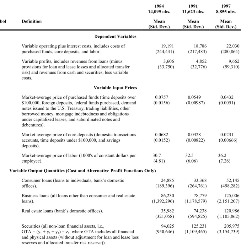
Table II gives the definitions of the variables in the cost and profit functions, their sample means, and standard deviations for 1984, 1991, and 1997. Although the continuous variables are generally expressed in natural logs in the cost and profit functions, we show means and standard deviations of the levels to be more informative. In choosing which financial accounts to specify as outputs versus inputs, we use the “asset approach” or “intermediation approach” (Sealey and Lindley 1977). All liabilities (core deposits and purchased funds) and financial equity capital provide funds and are treated as inputs, and all assets (loans and securities) use bank funds and are treated as outputs. Physical inputs (labor and premises) are specified as inputs that generate costs.8
[Table II goes here]
For the input and output prices, we specify the market-average price faced, rather than the actual price paid or received by the bank. As described in the notes to Table II, only data from other firms in the bank’s local markets are used to construct these market-average prices. The market-average prices faced are more likely to be exogenous to the bank than the prices actually paid or received by the bank. A second advantage is that any mistakes the bank makes in setting prices for its inputs or outputs given the market price conditions will be counted properly as inefficiencies, rather than just high or low prices or good or bad business conditions. For example, a bank that sets its deposit rate well above those of its market competitors, all else equal, will be measured as inefficient given its market-average deposit rate faced in the lnw vector. Market-average prices are also likely to average out some of the computational errors in measuring prices of individual banks.
The variable inputs for which prices lnw are specified are purchased funds, core deposits, and labor. The variable outputs lny are consumer loans, business loans, real estate loans, and securities, the latter category being measured simply as gross total assets less loans and physical capital, so that all financial assets are included. We specify off-balance-sheet items, physical capital, and financial equity capital as fixed netputs lnz. For the off-balance-sheet items, we use the Basel Accord risk weights on the assumption that the output may be roughly proportional to the perceived credit risk on which these weights are based. We specify these items as fixed primarily because of the difficulty of obtaining accurate price information. We also treat physical capital (premises and equipment) as a fixed input because it is slow to adjust and because it is difficult to measure prices for these durable inputs. Financial equity capital is an input under the asset approach, which we treat as fixed, in part because it is difficult to change quickly and in part because its price (the risk-adjusted expected return on equity) is difficult to measure. In addition, banks must meet regulatory capital requirements that may not be consistent with cost minimization or profit
maximization. It is important to include equity because it directly affects other costs and is an alternative source of funding for bank assets. It may affect the risk premium a bank pays for purchased funds, since equity provides a cushion against insolvency and an incentive to control risks (Hughes and Mester, 1998).9
Among the environmental variables lnv we include the log of the market-average nonperforming loans to total loans ratio, lnMNPL, and ½(lnMNPL) , since dealing with exogenous loan problems raises costs and lowers2 profitability. We use the market average rather than the individual bank’s ratio, since the market average captures the exogenous conditions in markets that affect loan performance. Market conditions are also accounted for by state income growth (STINC, ½STINC ). We specify controls for the state geographic restrictions on bank competition,2 including unit banking (UNITB), limited branching (LIMITB), with statewide branching as the base case; the degree of in-state holding company expansion permitted (LIMTBHC); whether out-of-state holding company expansion is prohibited (NOINTST); and the proportion of the U.S. banking assets held in states allowed to enter the bank’s own state (ACCESS, ½ACCESS ). We also include the Herfindahl index of local deposit market concentration (HERF);2 whether the bank is located in a metropolitan area (INMSA); and the identity of a bank’s primary federal regulator (FED, FDIC, with OCC as the base case).
5.2 Functional form
We use the Fourier-flexible functional form, a global approximation that includes a standard translog plus Fourier trigonometric terms. Our specification of the cost function is:
ln(C/w z ) = 3 3 " + 'i=12 $iln(w /w ) + ½ i 3 'i=12 'j=12 $ijln(w /w ) i 3 ln(w /w ) + j 3 'k=14 (kln(y /z )k 3
+ ½ 'k=14 'm=14 (kmln(y /z ) k 3 ln(y /z ) + m 3 'r=12 *rln(z /z ) + ½ r 3 'r=12 's=12 *rsln(z /z ) r 3 ln(z /z ) s 3
+ 'i=12 'k=14 0ikln(w /w ) i 3 ln(y /z ) + k 3 'i=12 'r=12 Dirln(w /w ) i 3 ln(z /z ) + r 3 'k=14 'r=12 Jkrln(y /z ) k 3 ln(z /z )r 3 + 'k=14 [Nk cos(q ) + k Tk sin(q )] + k 'k=14 'm=k4 [Nkm cos(q +q ) + k m Tkm sin(q +q )]k m
+ 'k=14 [Nkkk cos(q +q +q ) + k k k Tkkk sin(q +q +q )] + k k k 'n=114>nlnv + n lnu + C ln,C, (9) which is estimated separately for each year, allowing all the parameters to vary. The variables (y /z ), (z /z ), andk 3 r 3 MNPL (one of the environmental variables lnv) have 1 added before logging for every firm to avoid taking the log of zero. The q terms are rescaled values of thek ln(y /z ), such that each of the q is in the interval [0,2k 3 k B], where B here refers to the number of radians (not profits). The standard symmetry restrictions apply to the translog portion10
of the function (i.e., $ij = $ji, (km = (mk, *rs = *sr). We do not include factor share equations, which embody restrictions imposed by Shephard's Lemma or Hotelling’s Lemma, because these would impose the undesirable assumption of
no allocative inefficiency (i.e., no errors in responding to relative prices).11
The standard and alternative profit functions use essentially the same specification as the cost function with a few changes. First, the dependent variable for the profit functions replaces ln(C/w z ) with 3 3 ln[(B/w z ) +3 3 *(B/w z )3 3min* + 1], where *(B/w z )3 3 min* indicates the absolute value of the minimum value of (B/w z ) over all banks3 3 for the same year. Thus, 2t/*(B/w z )3 3 tmin* + 1 is added to every firm's dependent variable so that the natural log is taken of a positive number, since the minimum profits are typically negative. For the alternative profit function,12
this is the only change in specification (other than relabelling the composite error term as lnu + aB ln,aB), since the exogenous variables are identical to those for the cost function. For the standard profit function, the translog terms containing the variable output quantities, ln(y /z ), are replaced by the corresponding output prices, k 3 ln(p /w ), and thek 3 trigonometric terms containing the output quantities q are dropped.k
As shown, the cost, profit, and price terms are normalized by the last input price, the price of labor w , in3 order to impose linear homogeneity on the models. We also normalize the cost, profit, output quantities, and fixed13
netput quantities by the last fixed netput, financial equity capital z . Since the costs and profits of the largest firms3 are many times larger than those of the smallest firms, large firms would have random errors with much larger variances in the absence of the normalization, and division by equity should drastically reduce this heteroskedasticity. This normalization may also help reduce a bias toward finding high standard profit efficiency for the largest banks, since these banks may tend to have higher profits for a given set of prices, primarily because they were able to gain size over a period of decades, a feat that small banks cannot achieve in the short run. Division by equity may also give the dependent variables more economic meaning—the profit dependent variables become essentially the bank’s return on equity, or ROE (normalized by prices and with a constant added), a commonly accepted measure of how well the bank is using its scarce financial capital.
5.3 Methods used to decompose the total changes in costs and profits
We decompose the total changes in costs and profits over time, )TOTALCt,t+k, )TOTALBt,t+k, and )TOTALaBt,t+k in several steps. First, we estimate simple average-practice cost and profit functions for each year that include all banks whether they use best-practice versus inefficient techniques. The change in the average-practice functions over time reflects both the change in best practice (i.e., the change in f(@)) and the change in inefficiency (i.e., the change in lnu). We then use these average-practice functions to separate $ )TOTAL into the productivity change )PROD and the change in business conditions )BUSCOND components.
or profits from evaluating the average-practice function, holding business conditions constant at their period t levels. To see this, we rearrange the terms for )PRODCt,t+k from Eq. (4) above to give:
)PRODCt,t+k = {exp [fCt+k(X )] / exp [f (X )]} $Ct Ct $Ct C {exp[lnu$Ct+k] / exp[lnu ]}$Ct
= {exp [fCt+k(X )] $Ct C exp[lnu$Ct+k]} / {exp [f (X )] Ct $Ct C exp[lnu ]} .$Ct (10) The numerator is the predicted cost from the average-practice cost function from period t+k applied to the business conditions data from period t, and the denominator uses period t information for both the average-practice cost function and business conditions data. Put another way, cost productivity change includes the changes in best practice and inefficiency, both of which are incorporated in the average-practice cost function and holds business conditions unchanged. We simply use the estimated parameters of average-practice cost functions to evaluate the numerator and denominator of (10). We estimate the changes in costs or profits that are due to changes in business conditions as the changes in costs or profits that remain after accounting for the productivity changes (e.g., )BUSCONDCt,t+k is given by )TOTALCt,t+k /)PRODCt,t+k).
In general, the predicted costs or profits from the average-practice function evaluated at the average business conditions for that year and a zero random error term will not precisely equal the average total cost or profit for the industry because the transformations of the dependent variables to estimate the levels of costs or profits are nonlinear. We correct for this by multiplying the predicted levels from every average-practice cost or profit function by a constant, such that the predicted cost or profit at the mean value of business conditions for the year in which the function was estimated equals the sample average cost or profit for that year. In this way, our average-practice functions correctly predict the )TOTAL that they are being used to decompose, and the estimated )PROD and )BUSCOND correctly multiply to )TOTAL.
Finally, we decompose the productivity changes )PROD into the change in best practice )BESTPR and change in inefficiency )INEFF components. There is no consensus as to the best way to estimate the best-practice frontier. We use a version of the thick frontier method to measure )BESTPR (Berger and Humphrey, 1991). For each year, we divide up the banks based on their residuals from estimating the average-practice cost and profit functions. Banks with residuals in the “best” 25% in each of ten size categories (i.e., lowest cost residuals or highest profit residuals for their size category) are assumed to be best practice for that year. We then estimate the best-practice cost and profit functions using OLS on this most efficient quarter of banks. These estimated thick frontiers are treated as the best-practice functions f (C@), f (B@), and f (aB@). The 14 )BESTPR are measured as the changes in costs
or profits due to changes in f(@), holding business conditions constant at period t values. The changes in inefficiency )INEFF are estimated as the changes in productivity )PROD that remain after accounting for the change in best practice )BESTPR (e.g., )INEFFCt,t+k is estimated as )PRODCt,t+k /)BESTPRCt,t+k). Because of the uncertainty involved in the estimation of the thick frontier, the breakout of the change in productivity into its components should be considered less accurate than the other decompositions.
6. Main empirical results–Cost and profit changes for all U.S. banks, 1984-1997
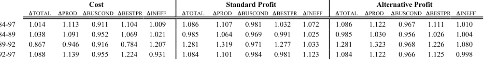
The top panel of Table III reports the total changes in costs and profits ()TOTAL), and the decompositions of these total changes into their )PROD, )BUSCOND, )BESTPR, )INEFF components for all U.S. banks over 1984-1997, and over the two subintervals 1984-1991 and 1991-1997.
[Table III goes here]
The )TOTAL figures show that the cost of the average bank rose at an annual rate of 1.1% over the entireC 1984-1997 interval, falling at an annual rate of 0.3% over the first seven years from 1984 to 1991, and rising at an annual rate of 2.7% over the subsequent six years from 1991 to 1997. These trends differ from those of the cost ratios shown in Table I above, which were scaled by equity or GTA. Here, we include these scale factors in our cost business conditions vector X . Financial equity capital is explicitly included in X as the third fixed netput (z ), andC C 3 GTA is implicitly included in X through the inclusion of its components, the asset output quantities plus the physicalC capital fixed netput (('k=14 y ) + z ). k 2
Using the average-practice cost function (estimated using all banks) to decompose the cost changes suggests that cost productivity worsened over both subintervals ()PROD > 1), while the business conditions as a wholeC reduced costs over both subintervals ()BUSCOND < 1). Moreover, these changes are accentuated and quiteC substantial in the 1991-1997 subinterval, with measured changes in productivity increasing costs at an annual rate of 12.5% and measured changes in business conditions lowering costs at an annual rate of 8.7%.
The strong benefits of these changes in business conditions in lowering costs are not at all surprising. As shown in Table II, interest rates on purchased funds and core deposits declined substantially during both subintervals. Given that interest expenses make up more than half of variable costs, it is expected that these declines in rates would reduce costs substantially. Somewhat offsetting these declines was the increase in the price of labor. The market-average price of labor, w , rose from $30.7 thousand in 1984 to $32.5 thousand in 1991 to $36.2 thousand in 1997.3 Financial equity capital (z ) grew by 5.1% on an annualized basis from 1984 to 1991 and 12.3% from 1991 to 1997,3
and GTA (('k=14 y ) + z ) grew by 3.7% and 8.3% per annum over the two subintervals, which helps explain why thek 2 cost ratios shown in Table I declined. As to the environmental variables, the decline in market nonperforming loans likely reduced the costs of dealing with these loans significantly, but the effects of liberalizations of state geographic restrictions on competition may either improve or worsen measured cost performance, as discussed further below. More puzzling are the measured unfavorable shifts in cost productivity of 4.2% of costs annually over 1984-1991 and 12.5% of costs annually over 1984-1991-1997. Using the best-practice cost function (i.e., using the “best” 25% of banks in each of ten size classes) suggests that both best-practice costs and inefficiency worsened in both subintervals and that an unfavorable shift in best practice explains most of the worsened productivity over the 1991-1997 subinterval (9.3 percentage points of the 12.5 percentage points). As noted, this breakout of the change in productivity into its components should be considered less accurate than the other decompositions, because of the uncertainty involved in the estimation of the thick frontier. Nonetheless, robustness checks using the best 15% and best 35% in each size class in place of the best 25% yielded qualitatively similar results.
These cost productivity/best practice deteriorations over time are in sharp contrast to the BLS annualized labor productivity improvements of 2.99% over 1984-1991 and 3.20% over 1991-1997, although other research studies of productivity change often found productivity deteriorations. Unlike the government statistics, our cost productivity measure controls for all of the output quantities, input prices, fixed netput quantities, and environmental conditions specified in the business conditions vector X . Our variable costs include noninterest expenses, whichC incorporate costs incurred elsewhere in the holding company in support of the bank.
Previous research cited the deregulation of deposit interest rates in the early 1980s and the resulting disequilibrium as important factors in worsening cost performance, but these factors almost surely cannot explain our worsening cost productivity/best-practice over 1991-1997, which is well after the deregulation of the rates. There may have been an increase in competition owing to liberalization of state geographic restrictions on competition or to exogenous market developments, which may make productivity/best practice appear to worsen because of a measurement problem in which the benefits to consumers are not taken into account in the cost function. However, it seems likely that these effects would be concentrated in the states that liberalized their rules the most and would largely be captured in the business conditions variables.15
The profit figures in the top panel of Table III show a dramatically different picture from the cost figures. The profit of the average bank rose at an annual rate of 7.9% over 1984-1997, and at annual rates of 4.3% and 12.2% over 1984-1991 and 1991-1997, respectively. The data suggest that the increase in profits is entirely due to
improvements in profit productivity—measured business conditions actually lowered profits slightly. The standard and alternative profit results differ as to whether the improvement in productivity is due to both improvements in best practice and better efficiency (standard profit result) or whether it is essentially all due to improvements in best practice (alternative profit result). Most important and striking, both profit approaches find substantial increases in productivity during 1991-1997—annual increases of 13.7% and 16.5% for standard and alternative profit, respectively—in sharp contrast to the cost productivity deterioration for this subinterval.
7. Potential explanations of the empirical results 7.1 Revenue-based productivity gains
This section tries to explain the striking finding that cost productivity worsened while profit productivity improved substantially over the 1991-1997 period. One likely explanation is revenue-based productivity gains. The cost approach and other approaches that do not consider revenues may not capture unmeasured changes in output quality over time or the profit maximization goal of banks, which requires that effort be spent to raise revenues as well as reduce costs. Efforts to raise quality may be measured as deteriorations in cost performance because these efforts raise expenditures, even if they increase revenues by more than the cost increases. The nonparametric concepts and the government statistics suffer from these weaknesses as well. Use of the profit approaches may help take into account unmeasured changes in the quality of banking services by including higher revenues paid for the improved quality, and may help capture the profit maximization goal by including both the costs and revenues.
Over time, banks have offered wider varieties of financial services, such as mutual funds, derivatives, and other products of financial engineering that help customers invest and manage risks. In addition, banks have provided additional convenience through more extensive branching and ATM networks, expanded availability of debit and credit cards, and a proliferation of online services. It seems likely that providing these new services and improving service quality significantly increased costs, but banks presumably made the necessary expenditures to maximize profits through higher prices or expanding or maintaining market shares. Our cost and profit productivity results are consistent with this hypothesis.
As noted above, the supernormal profits from adopting new technologies may persist over time in the industry if there is a series of innovations, as appears to have occurred in the banking industry. The early adopters of a successful new nonfinancial and financial technology earn supernormal profits from higher prices or increased market share, and others follow to avoid losing market share. The supernormal profits are competed away as the innovations become widely adopted. However, as long as the innovation process is ongoing, and different new technologies are
introduced at different points in time, innovating banks can keep earning high profits on different new or improved products. The early adopters of the series of new technologies may earn sufficient additional profits to raise the industry average for a considerable period, although the early adopters of different technologies need not consistently be the same banks.
As an example of how technology takes time to become adopted, consider small-business credit scoring, a set of statistical tools used to quantify and price risks. Prior to the mid-1990s, credit scoring was widely used in consumer lending, but it was little used in small-business lending for lack of a large loan database to develop a reliable model. Since 1995, however, small-business credit scoring models have become available from outside vendors that pool data from a number of banks (Mester, 1997). Credit scoring has been shown to be successful in16
increasing the small business loan market shares for the banks that have adopted it. Nonetheless, this technology is still in the process of adoption. As of January 1998, 37% of a sample of the largest banks in the U.S. still had not adopted small-business credit scoring, and this technology is still not used by most small banks (Frame, Srinivasan, and Woosley, 2001).
7.2 Selection of time intervals
We next consider the possibility that our findings may be driven by the way we have divided up the 1984-1997 period into two subintervals. To check for robustness, the bottom panel of Table III repeats the cost and profit change analysis of the top panel except the data are segmented into three intervals, 1984-1989, 1989-1992, and 1992-1997. The year 1989 was a relatively poor one for U.S. bank performance, and the 1989-1992 subinterval generally corresponds to what most consider to be the “credit crunch” period.17
The results shown in the bottom panel of Table III suggest that most of the main results are robust. Again, cost productivity worsens in the early and late time subintervals and again profit productivity improves over time, with cost worsening more and profits improving more in the 1990s than in the 1980s. However, the credit crunch subinterval 1989-1992 does differ in that cost productivity and best practice improve, while profit productivity and best practice improve much more than over any other subinterval. These unusual findings are reversed when the 1992-1997 subinterval is included along with the 1989-1992 subinterval—the worsening of cost productivity and best practice over 1992-1997 would more than overwhelm the improvements of 1989-1992. Overall, these data remain consistent with the hypothesis that banks’ goals over time were to maximize profits and that they provided additional services that raised costs but raised revenues even more. However, these data also suggest that the increased costs from producing higher-quality services may be temporarily overwhelmed by extreme improvements
in cost productivity.
7.3 Heterogeneity between small and large banks
Another potential candidate for explaining our results is the inclusion of both small and large banks in the same analysis. Small and large banks may provide different products that require use of different technologies. For example, a $1 billion loan issued by a large bank may be a different product requiring different monitoring and screening techniques than 10,000 loans of $100,000 each that may be issued (in aggregate) by small banks, but the balance sheet entries do not distinguish among these products. Also, it is likely that small banks and large banks adopt new technologies at different rates, and adapt to deregulation in different ways. To some extent, the observed effects thus far could reflect the shifting of banks into larger size classes over time, which may use different techniques to produce different products having different cost and profit characteristics.
To investigate this, we repeat the analysis for the smallest and largest quarter of banks in terms of GTA in each year, estimating separate cost and profit functions and using the average level of business conditions specific to each subsample. In 1997, the smallest quarter of banks ranges from about $1 million to about $33 million in assets and the largest quarter ranges from about $134 million to about $278 billion (all in 1994 dollars). The smallest quarter are unambiguously small, but the large quarter encompasses some medium-sized banks because there are not enough large banks alone to accommodate the number of parameters in the models.
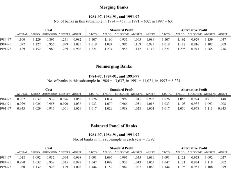
The results, shown in Table IV, suggest that our main results and conclusions about cost versus profit productivity are supported, but there are some interesting differences between small and large banks. Cost18
productivity worsens over the 1984-1991 and 1991-1997 subintervals for both small and large banks, particularly over the latter interval, supporting the earlier results. Using the other breakout of the time periods, the earlier finding of cost productivity improvement for the 1989-1992 credit crunch subinterval that is overwhelmed by cost productivity deterioration in the 1992-1997 subinterval is replicated only for the large-bank subsample. The earlier finding of profit productivity improvements in all cases is replicated here for all time subintervals. Overall, these19
data are again consistent with the hypothesis that banks attempted to maximize profits in part by providing additional services that raise revenues more than they raise costs.
7.4 Potential increase in risk-taking
Another potential explanation of our striking findings is that banks may have taken on additional risks during the boom period of the mid-to-late 1990s by shifting assets from securities to loans, by shifting from safer to riskier loans, by adding off-balance sheet risks, by becoming more highly levered, and so forth. Over the long run, higher risks may result in higher average portfolio returns (although not necessarily higher risk-adjusted returns), and these returns may have been magnified by the unexpected strength of the macroeconomy during this period, which may have provided “lucky” short-term rewards for the additional risk-taking. That is, an unusually high proportion of risky investments may have paid off and raised bank revenues as the strong U.S. economy allowed borrowers and other counterparties to repay an unexpectedly high proportion of their obligations. An increase in bank risk-taking that is not captured in our business condition variables, X and X , may be measured as a profit productivity increase,C B
even if there is no improvement in actual productivity.20
To evaluate this possibility, we first note that our business condition variables, X and X , do have a numberC B
of variables that are correlated with bank risk-taking, so we may have already controlled for much of any change in risk-taking. Both X and X include equity capital, off-balance activities, and market nonperforming loans to helpC B control for changes in bank leverage risk, off-balance sheet risk, and loan risk, respectively. In addition, X includesC the quantities of various types of loans and securities to help control for asset shifts and X includes the market pricesB of these assets to help control for the portfolio risks.
Banks might be taking increased risks in other ways not controlled for in our estimations. Nonetheless, virtually all raw-data indicators suggest that risk has not increased. The standard deviation of ROE fell from 0.0780 in 1991 to 0.0363 in 1997, and the standard deviation of ROA fell from 0.00501 to 0.00328 over the same period (Table I). Bank failures (not shown) also dropped precipitously from over 100 per year in the late 1980s and early 1990s to the single digits over the last few years of the sample. Under normal circumstances, these findings might suggest a decrease in risk, rather than an increase, although the unexpected strength of the macroeconomy makes it difficult to rule out entirely that such an increase in risk-taking occurred.21
7.5 Possible increase in conventional market power
Another possible explanation of the findings is that there was an increase in conventional market power over the 1991-1997 time period, in which product quality remained relatively constant, but banks exercised more market power in setting output prices. This could occur because of the consolidation of the banking industry over this time period. The increase in revenues from the higher output prices could explain the improvement in profit performance.
The worsened cost performance may also result in part from an increase in conventional market power, given that it has been found that banks in more highly concentrated local markets have lower cost efficiency, all else equal, presumably because of reduced managerial effort when competition is lax (Berger and Mester 1997, Berger and Hannan, 1998).
However, there are reasons to suspect this does not explain much of our findings. First, local market concentration changed little on average over time. The average value of HERF, the local deposit market concentration faced by banks, rose only about 1.6% from 0.2324 in 1991 to 0.2361 in 1997 (Table I). Despite the merger wave in banking, most of the activity appears to have been of the market-extension type that joined institutions in different local markets. Second, some recent research also suggests that the banks with persistently high profits22
in the 1990s are not consistently those with high measured market power (Berger, et al., 2000). In addition, both the X and X vectors of business conditions control for HERF, market-average input prices faced, and state geographicC B
restrictions on bank competition, and the X vector also controls for market-average output prices faced, althoughB prices are imperfectly measured. Thus, changes in market power would most likely be measured as the effects of changes in business conditions, rather than changes in productivity.
To investigate the conventional market power issue further, we run some additional regressions to estimate how changes in market concentration and other changes in competitive conditions in markets affected output prices. As shown in Table V, we regress the prices of each of the four variable outputs–consumer loans, business loans, real estate loans, and securities–on market concentration (HERF), the variables representing state geographic restrictions on competition (UNITB, LIMITB, LIMTBHC, NOINTST, and ACCESS, with STATEB excluded as the base case), and variables measuring the recent merger activity of the bank. The merger variables are dummies for whether the bank engaged in one or more mergers (i.e., absorbed one or more other bank charters) in the current year (MERGE0), prior year (MERGE1), or two years prior (MERGE2). These variables allow for the possibility that mergers result in dynamic changes in competition beyond their effects on HERF and the expected effects of the state geographic restrictions. The models are estimated over 1984-1997 with 163,547 observations. We then calculate the effects of the estimated changes in output prices on variable profits.
[Table V goes here]
The results suggest very little effect of market power increases on our profit performance results. The coefficients on HERF indicate that greater concentration is positively and statistically significantly related to the prices of business loans and securities, positively but insignificantly related to the price of real estate loans, and