Very High Resolution SAR Images and Linked
Open Data Analytics based on Ontologies
Daniela Espinoza-Molina,
Member, IEEE,
Charalampos Nikolaou, Octavian Dumitru, Konstantina Bereta, Manolis
Koubarakis, Gottfried Schwarz and Mihai Datcu,
Fellow, IEEE
Abstract—In this paper, we deal with the integration of multiple sources of information such as Earth observation Synthetic Aperture Radar (SAR) images and their metadata, semantic descriptors of the image content, as well as other publicly available geospatial data sources expressed as linked open data for posing complex queries in order to support geospatial data analytics. Our approach lays the foundations for the development of richer tools and applications that focus on Earth observation image analytics using ontologies and linked open data. We introduce a system architecture where a common satellite image product is transformed from its initial format into to actionable intelligence information, which includes image descriptors, metadata, image tiles and semantic labels resulting in an Earth observation-data model. We also create a SAR image ontology based on our Earth observation-data model and a 2-level taxonomy classification scheme of the image content. We demonstrate our approach by linking high resolution TerraSAR-X images with information from CORINE Land Cover, Urban Atlas, GeoNames, and OpenStreetMap, which are represented in the standard triple model of the RDFs.
Index Terms—TerraSAR-X images, Linked open data, queries, Strabon, ontologies, RDFs, analytics.
I. INTRODUCTION
Earth Observation (EO) imaging satellites continuously ac-quire huge volumes of high resolution scenes and increase the size of archives and the variety and complexity of EO image content. This exceeds the capacity of users to access the information content. In this context, it requires new method-ologies and tools, based on a shared knowledge from different sources, for locating interesting information in order to support emerging applications such as change detection, analysis of image time series, urban analytics, etc.
The state-of-the-art of operational systems for EO data ac-cess (in particular for images) allows queries by geographical location, time of acquisition or type of sensor [1]. Neverthe-less, this information is often less relevant than the content of a scene (e.g., specific scattering properties, structures, objects, etc.). Kato coined the term Content-based Image Retrieval[2] to describe his experiments on the automatic retrieval of images from a database by color and shape features. The term has since then been widely used for describing the process of retrieving desired images from large archives on the basis of low-level features such as color, texture, shape, etc. that can be automatically extracted from the images themselves. Several successful systems following this principle have been implemented during the last 20 years [3–7].
However, later the problem of matching the image content expressed as low-level primitive features with semantic defi-nitions, usually adopted by humans became evident; causing
the so-called semantic gap [8]. In an attempt to reduce the semantic gap, more systems including labeling or definition of the image content by semantic names were introduced. For example, [9] clarified the problem of the semantic gap and proposed several methods for linking the image content with semantic definitions. Here, it was demonstrated that the semantic representation has an intrinsic benefit for image retrieval by introducing the concept of query by semantic example (semantics and content). In general, an image archive contains additional information apart from the pixel raster data, as for example, distribution data, acquisition dates, processing and quality information, and other related information, which in general is stored and delivered together with the image data in the form of text files. However, this information is not fully exploited in querying the image archive. Thus, another important issue is how to deal with and take advantage of the additional information delivered together with EO images.
Presently, in addition to the image content and metadata, geo-information plays an important role in finding scenes of interest and projecting the results on a global view as a map representation. Thus, the tendency is to use geospatial information for querying and visualizing the content of image archives. In [10], Shahabi et al. presented a three-tier system for effectively visualize and query geospatial data. This system simulated geo-locations and fusion relevant geospatial data in a virtualized model in order to support decisions. It used a set of fundamental spatio-temporal queries and evaluated the queries to verify decisions virtually prior to executing them in the real world. This system was oriented to multimedia data. In [11], the geo-tags and the underlying geo-context for an advanced visual search were exploited showing satisfactory results in the image retrieval. The importance of integrating a geospatial infrastructure based on standardized web services into an EO data library was mentioned in [12]. The provision of a geospatial service infrastructure to access multilevel and multi-domain datasets is a challenging task. Stepinski et al.[13] discussed the lack of tools for data analytics, citing as an example the NLCD database, which has not been analyzed so far due to the lack of tools beyond basic statistics and SQL queries; thus, the authors introduced a new application called Land-ExA [13], which is a Geoweb tool for query and retrieval of spatial patterns in land cover datasets. This tool applies the concept of ”query by example” and, instead of presenting a ranked list of relevant maps, it produces a similarity map indicating the spatial distributions of the locations having patterns similar to the passed query. Brunner et al. presented a system implementing web-services and open-sources[14].
Here, an EO image is overlapped with vector sources via web services. It provides good visualization; however, no real image processing is achieved. Advanced queries using metadata, semantics and image content were presented in [15], showing how the integration of multiple sources helps the end-user in finding scenes of interest. Moreover, in recent years the development of ontologies as explicit formal specifications of the terms in the domain and relations among them [16] has been applied to the EO framework [17]. Knowledge mining in EO data archives based on an ontology was suggested by [18], which describes concepts and domains that can be adapted to EO understanding. In [19], a taxonomy for high resolution SAR images is proposed.
In this paper, we present a new framework that sets the foundations for the development of richer tools and appli-cations that focus on EO image analytics using ontologies and linked open data. The proposed framework allows a user to express complex queries by combining metadata of EO images (e.g., date and time of image acquisition), image content expressed as low-level features (e.g., selected feature vectors) and/or semantic labels (e.g., ports, bridges), as well as other publicly available geospatial data sources expressed in Resource Description Framework (RDF) as linked open data. The proposed framework also visualizes the results of such complex queries using geographical locations. We demon-strated our approach using Synthetic Aperture Radar (SAR) data, specifically very high resolution TerraSAR-X images as EO products, and CORINE Land Cover, Urban Atlas, GeoNames, and OpenStreetMap as geospatial data sources in the form of linked open data.
This paper is organized as follows. Section II describes our approach by presenting the system architecture. Section III presents the EO Data Model and defines the SAR image ontology. Section IV introduces query languages and shows some examples of queries based on geospatial ontologies. Section V presents some examples of urban analytics using queries based on ontologies. Finally, the conclusion and further work are presented in section V.
II. SYSTEMARCHITECTURE
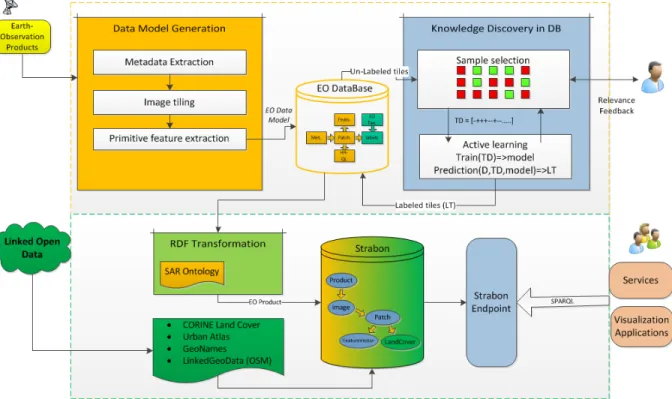
The system architecture is depicted in Fig. 1, which de-scribes the main components and the relations between them. The system is organized in two main parts 1) Processing of EO products which is in raster format and 2) Management of geospatial information which is in vector format. The system aims at providing an approach for linking EO image content expressed as semantic labels with the geometry of raster and vector objects that allows generation of analytic charts as the result of queries based on semantics, metadata, and related information.
The upper part of Fig. 1 is mainly focused on EO product processing by generating a data model and semantic de-scriptions based on knowledge discovery methods. The lower part is focused on the integration of geospatial data sources expressed in the form of linked open data and the answering and visualization of complex queries based on an ontology that models the EO domain and the processing of an EO product.
In the following, we start presenting the data sources man-aged by the system and later the description of each module.
A. Earth-Observation products and Linked Open Data
EO products together with linked open data are used as data sources in the system and they are described in the following:
1) Earth-Observation products: In general, EO images carry information about physical parameters and, additionally, present the Earth surface as matrices of pixels, where each pixel has an associated geographical location (latitude and lon-gitude). However, querying and accessing to EO images pose unique problems since geographical features to be represented as ontological objects are not defined in the structure of the data, which is a matrix of pixels. Moreover, EO images may be complemented with geospatial information in vector format, where the entities (objects) are well-defined with the basic elementary points, lines, and polygons. Vector data contain the geometry of these elements.
In this paper, we worked with TerraSAR-X images. A
TerraSAR-X product [20] is mainly composed of the image data and its metadata. The size of a very high resolution TerraSAR-X image is on average 10000×10000 pixels with varying numbers of bits per pixel(16 or 32), different types of data (float, unsigned int) and consisting of one or multiple bands in GeoTiff format, the corresponding metadata are con-tained in Extensible Markup Language (XML) files containing related information in form of structured text and numbers. An XML product description metadata file comprises about 250 entries grouped into categories such as product compo-nents, product information (i.e., pixel spacing, coordinates, format, etc.), processing parameters, platform data, calibration history, and product quality annotation. The image spatial resolution varies from 1 meter to 10 meters depending on the ordered product. A TerraSAR-X image has to be ordered in a selectable data representation, where four main alternative representations are available (Single look Slant range Complex (SSC), Multi-look Ground range Detected (MGD), Geo-coded Ellipsoid Corrected (GEC) and Enhanced Ellipsoid Corrected (EEC))
2) Linked Open Data (LOD): The use of linked data is a new research area which studies how one can make RDF data available on the Web, and interconnect it with other data with the aim of increasing its value for everybody [21]. In the last few years, linked geospatial data has received increased attention as researchers and practitioners have started tapping the wealth of geospatial information available on the Web. As a result, the linked open data cloud has been rapidly populated with geospatial data (e.g., OpenStreetMap) some of it describing EO products (e.g., CORINE Land Cover, Urban Atlas). The abundance of this data will become useful to EO data centers to increase the usability of the millions of images and EO products that are expected to be produced in future.
In the following, we describe the EO products CORINE Land Cover and Urban Atlas that we have made available in RDF as linked geospatial data at the Datahub portal1 and
Fig. 1:Architecture of the system. The system is composed of (upper-part) Earth observation product processing and (lower-part) management of geospatial information.
other useful publicly available linked geospatial datasets, such as OpenStreetMap and GeoNames.
a) CORINE Land Cover: The CORINE Land Cover (CLC) project is an activity of the European Environment Agency (EEA) that collects data describing the land cover of 38 European countries. The project uses a hierarchical scheme with three levels to describe land cover with a mapping scale of 1:100,000 and a small mapping unit of 25 hectares. Level 1 is the most generic classification (e.g., artificial surfaces, agriculture areas) and comprises 5 categories, level 2 (e.g., ur-ban fabric, industrial, transport units) comprises 15 categories, and the last level is the most detailed one (e.g., continuous urban fabric, discontinuous urban fabric) comprising around 45 categories.
b) Urban Atlas: Urban Atlas (UA) is also an activity of the EEA that provides reliable, inter-comparable, high resolution land use maps for 305 large European urban zones and their surroundings. Its geometric resolution is 10 times higher (1:10,000) than that of CLC with a minimum mapping unit of 0.25 hectares for urban areas and 1 hectare for other areas. The project uses a four-level hierarchical scheme based on the CLC nomenclature. The first level comprises 4 cate-gories (e.g., forests, water, artificial surfaces), the second level comprises 4 categories (e.g., commercial units, mines, dump and construction sites), the third level comprises 12 categories (e.g., discontinuous urban fabric, sports and leisure facilities, airports), while the fourth level comprises 7 categories (e.g., fast transit road and associated land). The Urban Atlas is available for more than 150 urban agglomerations within Europe.
We stress that the CLC and UA datasets present
comple-mentary characteristics making them very attractive to an EO expert who can combine them for performing analytical tasks, such as the ones presented in Section V. Fig. 2 depicts exactly this observation where the content of the CLC and UA datasets is depicted for the region of Cologne, Germany. One can access various kinds of metadata information for the areas classified by either CLC or UA, such as its computed area, its code, the date of production, as well as its land use/land cover.
c) OpenStreetMap: OpenStreetMap2(OSM) maintains a
global editable map based on information provided by users, which is organized according to an ontology derived mainly from OSM tags, i.e., attribute-value annotations of nodes, ways, and relations. The OSM data have been transformed into RDF and published as linked open data by the LinkedGeoData project (http://linkedgeodata.org/).
d) GeoNames: GeoNames3 is a gazetteer that collects
both spatial and thematic information for various place names around the world. It contains over 10 million geographical names and consists of over 8 million unique features whereof 2.8 million populated places and 5.5 million alternate names. All features are categorized into one out of nine feature classes and further sub-categorized into one out of 645 feature codes. GeoNames is integrating geographical data such as names of places in various languages, elevation, population and others from various sources.
2http://openstreetmap.org/ 3http://www.geonames.org/
B. Earth Observation product processing
The upper part of Fig. 1 shows the modules used for EO product processing. This part is composed of 1) Data Model Generation (DMG), 2) EO DataBase (EO-DB) and 3) Knowledge Discovery (KD).
1) Data Model Generation: The DMG aims at transform-ing from an initial form of full EO products to actionable intelligence information, which includes image descriptors, metadata, image patches, etc., called EO Data Model as depicted Fig. 3. Finally, all this information is stored into a relational database enabling the rest of the modules. During DMG the metadata of an EO image is processed. In general, the metadata comes in a text format stored as markup language (e.g., XML) files including information about the acquisition time, the quality of the processing, description of the image like resolution, pixel spacing, number of bands, origin of the data, acquisition angles, acquisition time, resolution, projec-tion, etc. The use of metadata enriches the data model by adding more parameters that can be used later in advanced queries. Then the EO image is going to be cut into square-shaped patches and for each patch a very high resolution quick-look is generated. These quick-looks are used in the knowledge discovery component. In a next step, using the patches, the image content analysis is performed by different feature extraction methods, which are able to describe texture, color, spectral features, etc. Currently, the system relies on two feature extraction methods, namely, the Gabor Linear Moment and Weber Local Descriptors.
a) Gabor Linear Moment (GLM): GLM is a linear filter used in image processing. Frequency and orientation representations of a Gabor filter are similar to those of the human visual system, and it has been found to be particularly appropriate for texture representation and discrimination [22]. In the spatial domain, a 2D Gabor filter is a Gaussian kernel function modulated by a sinusoidal plane wave. Gabor filters are self-similar; all filters can be generated from one mother wavelet by dilation and rotation. The implementation of the Gabor filter by [22] convolves an image with a lattice of possibly overlapping banks of Gabor filters at different scales, orientations, and frequencies. The scale is the scale of the Gaussian used to compute the Gabor wavelet. The texture parameters computed from the Gabor filter are the mean and variance for different scales and orientations. The dimension of the final feature vector is equal to twice the number of scales multiplied by the number of orientations; for instance, using two scales and six orientations results in a feature vector with 24 elements.
b) Weber Local Descriptor (WLD): Inspired by Webers law, Chen et al.[23] proposed a robust image descriptor for texture characterization in optical images with two compo-nents: differential excitation and orientation. The differential excitation component is a function of the ratio between two terms: 1) the relative brightness level differences of a current pixel compared to its neighbors and 2) the brightness level of the current pixel. The orientation component is the gradient orientation of the current pixel. Using both terms, a joint histogram is constructed giving the WLD descriptor as a result. This filter was adapted for SAR images [24]. Here,
the gradient in the original WLD was replaced by the ratio of mean differences in vertical and horizontal directions.
As result of the DMG, part of theEO Data Modelis created and stored into the database. This model will be completed by using active learning methods for semantic labeling of the image content and posteriori it will be complemented with geospatial information coming from linked open data sources.
2) Earth Observation database: The EO product process-ing is centered on a relational database management system (DBMS), where the database structure supports the knowledge discovery component after mapping theEO Data Modelinto several tables and creating the relations between them. The use of a DBMS provides some advantages such as the natural integration of the different kinds of information, the ensuring of the referential integrity, the speed of the operations, etc. Therefore, all the information about the EO product such as patches with geographical locations, image coordinates, meta-data entries, extracted features, quick-looks, etc. are stored into a structured table-based scheme, which implements the proper relations between the tables and indices for performance optimization.
3) Knowledge discovery: The knowledge discovery com-ponent deals with finding hidden patterns or existing objects in the EO database and grouping them in semantic categories by involving the end-user interactively for labelling the image content. The image labeling or semantic definition is based on active learning methods being supported, as for example, by a Support Vector Machine (SVM). Starting from a limited number of labeled data, active learning selects the most informative samples to speed up the convergence of accuracy and to reduce the manual effort of labeling [25]. The two core components in active learning are the sample selection strategy and model learning, which are repeated until convergence. In our implementation of the sample selection (cf. Fig. 1), a set of image patches are presented to the end-user, who will give positive and negative feedback examples assuming that a positive example is a patch containing an object of interest. Later, the list of positive and negative samples is passed as training data (TD) to a support vector machine. The SVM creates a model based on the training data, using this model it will be able to predict whether another patch belongs to the desired category or not. At the beginning of the procedure, when only a few labeled tiles are available, a coarse classifier is learned. After that, we repeat the iteration of the two components until the classification result is satisfactory. The number of iterations is determined by the end-user, who will stop the interactive loop when he is satisfied with the results. These results are grouped as a new category with a semantic label given by the end-user. Thus, this component adds semantic descriptors to theEO Data Model.
C. Management of geospatial information
The lower part of Fig. 1 is responsible for enriching EO products with auxiliary data as for example land cover cate-gories taken from CORINE Land Cover (CLC), geographical location of points taken from Geonames, etc. These offer querying functionalities to users that go beyond the ones
currently being available to them. This can be done by relying on semantic web technologies, such as stRDF and stSPARQL, OWL ontologies, and geospatial data sources expressed as linked data.
The enrichment of EO products stored in the EO database involves first a transformation step of the relational database encoding to the data model RDF. This transformation is guided by an OWL ontology that models the EO domain and the knowledge pertaining to the processing of an EO product as it was previously described. This ontology is hereinafter called
SAR ontology. The result of the transformation is the RDF description of the EO products, which is subsequently stored in a Strabon RDF store together with other available linked open data, such as CLC. The Strabon endpoint component is the interface that provides user access to the content of Strabon by allowing users to formulate complex queries in the stSPARQL query language. The Strabon endpoint also offers capabilities to visualize the results of complex queries on a map and diagrams that are useful for data analytics. An important part of our architecture is that it allows the users also to leverage the linked data offered by the Strabon endpoint and to develop domain-specific services (e.g., data mining, rapid mapping) as well as general-purpose applications (e.g., visualization tools, such as [26]).
(a) A map centered on the region of Cologne depicting avail-able information from the CORINE Land Cover dataset
(b) A map centered on the region of Cologne depicting available information from the Urban Atlas dataset
Fig. 2: (a) CORINE Land Cover and (b) Urban Atlas information for the region of Cologne.
III. EODATA MODEL ANDSARONTOLOGY
After the processing of EO products, a data model is gener-ated in order to provide all information representing actionable
Fig. 3:UML Representation of theEO Data Model.
intelligence that later is exploited for semantic definition of the image content. In a further step, the description of the EO products is made by using RDFs and ontologies.
A. EO Data Model
The EO data model has been introduced in [15]. Here, we present an enhanced and extended version of this model including semantic annotations as is depicted in Fig. 3.
The EO Data Model represents an EO product, which is composed of metadata, a raster image, and vector data. The raster image is divided into patches, which are converted to feature vectors by applying feature extraction methods. Later, using machine learning methods, the patch content is associated with semantic labels (categories) giving as result a semantic catalogue of the image. From this model, the main processing unit is a patch because it consists of geographical information, it has associated feature vectors, and it includes semantic definitions. This data model is transformed to the standard triple model of the RDF in order to be part of the SAR ontology and to be linked to other data as for example CORINE Land Cover (CLC), Urban Atlas (UA), etc.
B. Definition of the SAR ontology
In order to define the SAR ontology, the semantic annotation of the SAR image content is organized as two-level hierarchi-cal taxonomy which later is used as a main component of the ontology. In this section we define theSAR ontologybased on ourEO Data Model and the TerraSAR-X taxonomy.
1) TerraSAR-X taxonomy: The TerraSAR-X taxonomy is the result of a careful analysis and annotation of the content of SAR images [19]. A sufficiently large dataset composed of several TerraSAR-X scenes was created in order to perform the annotation on a large set of TerraSAR-X data. The acquisition of TerraSAR-X products covers109different areas around the world. The total number of patches obtained after running the data model generation is about 110,000 and these patches were classified into about850 semantic categories. For these categories about 75 independent labels were defined and we grouped these labels into a hierarchical semantic annotation
scheme [27]. The annotation was made using the machine learning methods described above. Our scheme is a two-level annotation scheme where level 1 gives general information about the content of a patch (e.g., agriculture, bare ground, forest, transportation, unclassified, urban area, or a water body), while level 2 details the general information from level
1 (e.g., for forest − > forest broadleaf, forest coniferous, forest mixed, parks, trees, and not specified further).
EO Taxonomy Agriculture Cropland Pasture Water bodies Rivers ... Transportation Roads Ports ....
Fig. 4: Taxonomy scheme with two levels: Level 1 gives general information about the categories and level 2 details each category of level 1.
Fig. 4 presents only few examples of the taxonomy defined for TerraSAR-X during the annotation procedure. The com-plete TerraSAR-X taxonomy is presented in detail in [27]. Examples of the image content are presented in Fig. 5. Here, we selected TerraSAR-X patches representing 6 major lan-duse classes (urban area, forest, water bodies, transportation, agriculture and bare ground). In Fig. 5 can be seen that urban area classes are the classes with very high brightness. Semantic class forest has medium brightness and homogeneous texture. The brightness varies according to the thickness of vegetation. Roads appear as dark linear features and class ocean appears as dark pixels in the TerraSAR-X image.
Fig. 5: (left-right) high density urban area, forest broadleaf, ocean, pasture, skyscraper, road, lake, and bridge.
In the following, the SAR ontology derived from our TerraSAR-X taxonomy is described
2) SAR ontology: The description of the EO products follows the OWL ontology4depicted in Fig. 6 and which will be referred as the SAR ontology. It comprises the following major parts:
1) the part that comprises the hierarchical structure of a product and the XML metadata associated with it (e.g., time and area of acquisition, sensor, imaging mode, incidence angle),
4http://www.earthobservatory.eu/ontologies/dlrOntology.owl
Fig. 6: The SAR ontology based on the two-level classification scheme defining the semantic categories of TerraSAR-X images.
2) the part that defines the concepts and properties that formalize the outputs of the data model generation com-ponent (e.g., patch, feature vector),
3) the part that defines the land cover/use classification scheme for annotating image patches that was con-structed while experimenting with the knowledge discov-ery framework presented above (e.g., ’port’, ’urban built-up’).
In particular, the SAR ontology comprises the following classes (as shown in Fig. 6).
• Image. This class corresponds to TerraSAR-X satellite images. Instances of this class are TerraSAR-X images.
• Product. This class corresponds to EO products that are associated with TerraSAR-X images. An instance of the class Product might be associated with multiple instances of the classImage through the propertyhasImage.
• Metadata. This class corresponds to TerraSAR-X xml annotation file. Instances of this class are TerraSAR-X metadata entries.
• Patch. This class corresponds to patches of an image as they are generated using the tiling procedure mentioned in Section II-B1. Instances of this class are associated with instances of the classImage through the property hasImage.
• FeatureVector. This class corresponds to a feature vector that is computed for a specific patch. An instance of this class is a feature vector value for an instance of thePatch class with which it is associated through the propertyhasFeatureVector.
• LandCover. This class corresponds to the land cover/land use of a geographical area that a patch occu-pies. TheLandCoverclass has a number of subclasses based on the classification scheme of Fig. 4, which is reflected in the SAR ontology.
• Label. This class corresponds to the semantic label that is assigned to a patch through the propertyhasLabel. Instances of the class Label are associated with sub-classes of the class LandCover through the property correspondsTo.
IV. QUERY LANGUAGES A. Standard Query Languages
Using theEO Data Modelstored in the relational database, we can access the information via Standard Query Language (SQL) statements. SQL is a statement based logical query lan-guage, which allows finding and exploiting data in a standard manner. SQL statements allow us to easily query an image archive combining all defined entities and their attributes. For example, a typical SQL statement for searching EO products within in a specific time period is
SELECT resolution, startimeutc, stoptimeutc FROM metadata
WHERE starttimeutc > 30/06/2007 and stoptimeutc <30/06/2010.
This query returns the EO images acquired during this period. More complicated queries can be performed based on SQL statements as for example:
SELECT * FROM patch
WHERE mean(gabor-features)>45.
A list of patches with a mean value of their extracted features being greater than 45 is returned.
From an application point of view, this kind of queries is a powerful tool in finding information in the relational database.
B. The data model stRDF and the query language stSPARQL
The stRDF data model and the stSPARQL query language are extensions of the RDF data model and the SPARQL query language for the representation and querying of RDF data with geospatial information. stRDF introduces the new data typestrdf:geometryfor modeling geometric objects that change over time. The values of this data type are typed literals that encode geometric objects using the OGC standard Well-known Text (WKT) or Geographic Markup Language (GML). In stRDF, information is expressed as triples of URIs, literals, and blank nodes in the form ”subject predicate object”. stRDF allows triples to have an optional fourth component representing the time the triple isvalid in the domain.
The following four RDF triples encode information related to a patch of an image. The prefix tsx corresponds to the namespace for the URIs that refer to the SAR ontology, while xsdandstrdfcorrespond to the XML Schema namespace and the namespace for our extension of RDF, respectively.
tsx:QKL_TSX1_SAR...047_160_0_0.jpg a tsx:Patch; tsx:hasSize "160"ˆˆxsd:integer;
tsx:hasIndexI "0"ˆˆxsd:integer;
strdf:hasGeometry "POLYGON((12.28 45.45,..., 12.28 45.45))"ˆˆstrdf:WKT.
The fourth triple above shows the use of spatial liter-als to express the geometry of the patch in question. This spatial literal specifies a polygon that has exactly one ex-terior boundary and no holes. The exex-terior boundary is se-rialized as a sequence of the coordinates of its vertices. These coordinates are interpreted according to the WGS84 geodetic coordinate reference system identified by the URI http://spatialreference.org/ref/epsg/4326/ (which can be omitted from the spatial literal).
stSPARQL provides functions that can be used in filter expressions to express qualitative or quantitative spatial rela-tions. For example, the function strdf:containsis used to encode the topological relation non-tangential proper part inverse (NTPP−1) of RCC-8 [28]. stSPARQL also supports
update operations (insertion, deletion, and update of stRDF triples) on stRDF data in SPARQL Update 1.15. In addition,
stSPARQL performs the corresponding spatial selection and spatial join by instantiating the two queries templates.
The following query, expressed in stSPARQL, computes the distribution of instances of Urban Atlas classes in TerraSAR-X images.
SELECT ?uaLandUse (COUNT(DISTINCT ?ua) AS ?count) WHERE {
?ua ua:hasCode ?uaCode . ?ua ua:hasLandUse ?uaLandUse . ?ua geo:hasGeometry ?uaGeometry. ?uaGeometry geo:asWKT ?uaGeo . #Berlin FILTER (strdf:mbbIntersects(?uaGeo, "POLYGON((13.317529 52.494114000000003,13.4 29790499999999 52.50573,13.416467000000001 52.554319999999997,13.303621 52.54265600000 0001,13.317529 52.494114000000003))" ˆˆstrdf:WKT)) . } GROUP BY ?uaLandUse ORDER BY DESC(?count)
In the above query, linked data from Urban Atlas are used to retrieve geospatial information about a TerraSAR-X scene taken over Berlin, Germany. Thestrdf:mbbintersects function checks whether the minimum bounding box of the geometry of each Urban Atlas class intersects with the min-imum bounding box of the polygon that represents the given TerraSAR-X image of Berlin. We realize that stSPARQL enables us to develop advanced semantics-based querying of EO data along with open linked data being available on the web. In this way, the architecture of Fig. 1 unlocks the full potential of these datasets, as their combination the abundance of data being available on the web is offering significant added value.
The stRDF model and stSPARQL query language have been implemented in the Strabon system which is freely available as open source software6. Strabon extends the well-known
open source Sesame 2.6.3 RDF store and uses PostGIS as its spatially-enabled backend DBMS.
V. GEOSPATIAL DATA ANALYTICS
In the following experiments, we use a test dataset com-posed of 200 worldwide TerraSAR-X scenes, where 109 images were applied to the formulation of the SAR Ontol-ogy described above. In most examples, we interpret three TerraSAR-X scenes taken over Germany (Berlin, Munich and Cologne) since CORINE Land Cover and Urban Atlas data are available for these cities. We also use Geonames data. It is important to mention that applications are able to link to
5http://www.w3.org/TR/sparql11-update/ 6http://www.strabon.di.uoa.gr/
TABLE I: Number of patches, in the area of Cologne, that are attributed to specific categories according to the SAR ontology. SELECT ?annotation
(COUNT(DISTINCT ?patch) AS ?count) WHERE {
?patch rdf:type tsx:Patch .
?patch geo:hasGeometry ?patchGeom . ?patchGeom geo:asWKT ?patchWKT . ?patch tsx:hasLabel ?label . ?label tsx:type tsx:Label .
?label tsx:correspondsTo ?annotation . #Cologne FILTER (strdf:mbbIntersects(?patchWKT, "POLYGON((6.915 50.914, 7.025 50.927, 7.012 50.972, 6.903 50.96, 6.915 50.915, 6.915 50.914))"ˆˆstrdf:WKT)) . } GROUP BY ?annotation ORDER BY DESC(?numberOfPatches)
TABLE II: Distribution of semantic categories over Cologne city according to TerraSAR-X, CLC, UA and Geonames
Dataset Total 1st Category 2nd Category TSX 27 16% High density Ur-ban Area 14% H.dRoads.UA and CLC 9 22% Industrial and
commercial Area 20% Green areas UA 14 57.1% Continuous urbanfabric 17% Industrial
GeoN 6 84% S 9.1% P
different data sources and to use and share data effectively for answering queries and supporting specific requirements by the use of RDFs.
A. Semantic link between geospatial ontologies
By exploiting the expressivity of the query language SPARQL and the capability of Strabon Endpoint to export query results encoded into various formats (XML, CSV, KML, etc.), or to visualize them as diagrams, users can explore implicit properties about data.
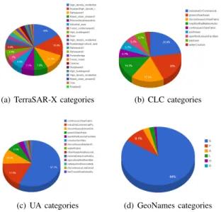
For example, an interesting question is: ”What is the dis-tribution of TerraSAR-X semantic categories in a specific area?. This can be answered by the query in Table I, which counts how many unique patches, in the area of Cologne, are attributed to specific TerraSAR-X categories. By posing similar queries for the CLC, UA and GeoNames datasets and by visualizing the results as pie charts (cf. Fig. 7) a user can have an insight for the category distribution of each dataset. We observe that the TerraSAR-X and CLC datasets have a high diversity of categories being almost uniformly distributed among the patches, while UA and GeoNames have less diversity of categories and one or two categories are attributed to almost every patch. Table II summarizes the results of the Fig. 7; here, it can be seen that TerraSAR-X has the highest number of semantic categories, where 16% of the patches are classified as ’High density urban area’.
SPARQL can also be used to correlate different datasets and to discover similarities or conflicts between them. For example, the query in Table III selects all CLC categories which are attributed to patches labeled as ’Industrial area’ in the SAR ontology. Table IV summarizes the results. Here, we observed that the category ’industrial area’ in the SAR
(a) TerraSAR-X categories (b) CLC categories
(c) UA categories (d) GeoNames categories Fig. 7:Categories of different datasets (TSX, CLC, UA, GeoNames) for the city of Cologne.
TABLE III:Select all CLC categories which are attributed to patches labeled as ’industrial area’ in theSAR ontology.
SELECT DISTINCT ?annotation ?clcLandUse WHERE {
?patch rdf:type tsx:Patch .
?patch geo:hasGeometry ?patchGeom . ?patchGeom geo:asWKT ?patchWKT . ?patch tsx:hasLabel ?label . ?label rdf:type tsx:Label .
?label tsx:correspondsTo tsx:Industrial_area. ?clc clc:hasID ?clcID .
?clc clc:hasLandUse ?clcLandUse . ?clc geo:hasGeometry ?clcGeom. ?clcGeom geo:asWKT ?clcWKT .
FILTER (strdf:contains(?clcWKT, ?patchWKT)) . #Cologne
FILTER (strdf:mbbIntersects(?clcGeo, "POLYGON ((6.915 50.915,7.025 50.927,7.012 50.972,6.903 50.960,6.915 50.915))"ˆˆstrdf:WKT)) }
ontology is also characterized as Industrial area in CLC and UA; however, more semantic categories are found in both datasets.
Finally, we can use SPARQL to discover statistic properties by correlating different datasets. For example, the query in Table V counts how many patches with a specific label in the area of Munich are characterized as ’Continuous urban fabric’ according to the CLC dataset. The results of this query and
TABLE IV:CLC, UA and GeoNames categories attributed to patches labeled as ’industrial area’ in theSAR Ontology
CLC UA GeoNames
Industrial or Commer-cial units
Other roads and asso-ciated land S Continuous urban
fab-ric
Continuous urban
fab-ric A
Discontinuous urban
fabric Green urban areas Industrial commercial public military and private units
TABLE V: Count how many patches in the area of Munich with a specific label are contained in an area characterized as ’Continuous urban fabric’ according to the CLC dataset
SELECT ?annotation
(COUNT(?patch) AS ?count) WHERE {
#select corine areas ?clc a clc:Area .
?clc clc:hasLandUse clc:continuousUrbanFabric . ?clc geo:hasGeometry ?clcGeom .
?clcGeom geo:asWKT ?clcWKT . #select patches
?patch rdf:type tsx:Patch .
?patch geo:hasGeometry ?pathcGeom . ?patchGeom geo:asWKT ?patchWKT . ?patchWKT tsx:hasLabel ?label . ?label tsx:correspondsTo ?annotation . #Munich
FILTER (strdf:mbbIntersects(?patchWKT, "POLYGON((11.492 48.110,11.599 48.123,11.586 48.169,11.479 48.157,11.492 48.110))"ˆˆstrdf:WKT)) . FILTER (strdf:contains(?clcWKT, ?patchWKT)) . }
GROUP BY ?annotation
ORDER BY DESC(?numberOfPatches)
Fig. 8: How many patches with a specific label are contained in a continuous urban fabric area (CLC)?.
two similar ones about Cologne and Berlin are visualized as a histogram in Fig. 8. These queries select patches in continuous urban fabric CLC areas. Thus, the TerraSAR-X categories that are selected are similar (e.g., different types of residential areas and high building areas). In Fig. 8 we can also see that the largest number of ’high residential area’ patches occur is in Munich. The number of ’roads’ is similar in Berlin and Cologne.
B. Land use distributions
In the following examples, we present land use distributions of the different geospatial datasets.
a) Land use distribution of the whole dataset: Fig. 9 shows the land use distribution of the whole dataset according to the SAR Ontology. As we can see, around 34 different land use categories can be identified, with ’medium density residential area’ ranking first, followed by ’roads’ and ’high density residential area’.
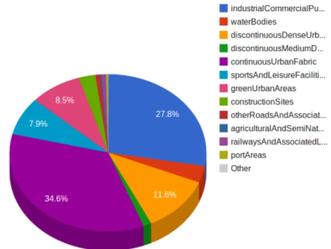
b) Land use of Berlin: Fig. 10 shows the land use distri-bution of Berlin according to the Urban Atlas dataset. The pie
Fig. 9:Land use distribution of our test dataset.
chart visualizes the result of the stSPARQL query described in the previous section. As we can see, the ’continuous urban fabric areas’ cover the highest percentage of land use in Berlin followed by ’water bodies’.
Fig. 10:Land use distribution of Berlin according to Urban Atlas.
c) Land use of Munich: In this example, we look for semantic categories within an area of Munich characterized as ’continuous urban fabric’. The query shown in Table VI discovers the semantic categories of the SAR ontology that correspond to the ’continuous urban fabric areas’ of Munich according to the CORINE Land Cover dataset. The result of the query is visualized in Fig. 11. Here, we can observe that categories like ’high density residential area’, ’sport area’, forest’, channel’, etc. which belong to the SAR ontology are characterized as ’continuous urban fabric’ in the CLC dataset.
d) Land Use of Cologne: In this example, we analyzed the number of Urban Atlas areas of Cologne contained by a TerraSAR-X patch. The query specification is described in Table VII. Here, this returns the number of Urban Atlas areas that exist in each TerraSAR-X patch of Cologne city. The result is shown in Fig. 12.
C. Urban analytics
Queries help us to get an idea about the existing semantics that are in the database and the relation between these
seman-TABLE VI:Count how many patches in the area of Munich with a specific label are contained in an area characterized as ’Continuous urban fabric’
SELECT ?annotation (COUNT(DISTINCT ?l) as ?count) WHERE { ?p rdf:type tsx:Patch . ?p geo:hasGeometry ?tsxGeometry . ?tsxGeometry geo:asWKT ?g . ?p tsx:hasLabel ?l . ?l rdf:type tsx:Label . ?l tsx:correspondsTo ?annotation . ?clc clc:hasID ?clcID . ?clc clc:hasLandUse clc:continuousUrbanFabric . ?clc geo:hasGeometry ?clcGeometry.
?clcGeometry geo:asWKT ?clcGeo .% #Munich FILTER (strdf:mbbIntersects(?clcGeo, "POLYGON((11.4923935 48.110413000000001, 11.599087000000001 48.123100000000001, 11.586228999999999 48.169327000000003, 11.479395999999999 48.156627999999998, 11.4923935 48.110413000000001))" ˆˆstrdf:WKT)) . FILTER (strdf:contains(?clcGeo, ?g)) . } GROUP BY ?annotation ORDER BY DESC(?count)
Fig. 11:Semantic categories of the SAR ontology within an area of Munich characterized as continuous urban fabric.
Fig. 12: Number of Urban Atlas areas of Cologne contained in a specific patch.
tics and other different parameters (e.g., location of the scene, incidence angles, etc.).
e) Cities ranked by green areas: Fig. 13 shows the cities of our experimental database ranked by green areas. The bar chart illustrates the distribution of green areas by city. A query was performed using semantic labels like ’trees’, ’forest’, ’parks’ and we counted the total number of patches belonging to these categories. The results highlighted that the city code
TABLE VII: Number of Urban Atlas areas of Cologne being contained in a TerraSAR-X patch
SELECT ?annotation (COUNT(?ua) AS ?numOfUAreas) WHERE {
#select Urban Atlas areas ?ua ua:hasLandUse ?uaLandUse . ?ua geo:hasGeometry ?uaGeometry . ?uaGeometry geo:asWKT ?uaGeo . #select patches ?p rdf:type tsx:Patch . ?p geo:hasGeometry ?tsxGeometry . ?tsxGeometry geo:asWKT ?g . ?p tsx:hasLabel ?l . ?l tsx:correspondsTo ?annotation . #Cologne
FILTER (strdf:mbbIntersects(?g, "POLYGON ((6.9154109999999998 50.914684000000001, 7.0246969999999997 50.926659999999998, 7.011908 50.972445999999998, 6.9025806999999997 50.960479999999997, 6.9154109999999998 50.914684000000001))" ˆˆstrdf:WKT)) .
FILTER (strdf:contains(?g, ?uaGeo)) . }
GROUP BY ?annotation
Fig. 13:Cities ranked by green areas.
59, referring to Teica in Romania, has the highest percentage of green areas.
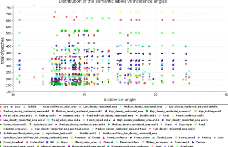
f) Distribution of semantic labels by incidence angle:
In this kind of query, we used metadata and semantic labels in order to show the distribution of semantic labels versus incidence angle and we analyzed whether there is a correlation between them. Fig. 14 shows the results. Here, it can be observed that most of the semantic labels appear at incidence angles between 35 and 40; however, the category ’forest’ occurs at angles of more than 45.
g) Distribution of water bodies by continents: In this kind of query, we used Geonames and semantic categories from theSAR ontology in order to group our scenes according to the place and to semantic labels being associated with water bodies (e.g., channels, rivers, ocean, etc.). Fig. 15 shows the results. One can see that the member states of the European Union have the highest diversity in water bodies linked to 23 different semantic categories, where the major category corresponds to ’river and stubble’. Oceania has only three water body classes. ’Channels’ exist in five continents, while the category ’river and agriculture’ does not exist in North America and Oceania
Fig. 14:Distribution of semantic categories by incidence angle.
Fig. 15:Distribution of water bodies by continent.
VI. CONCLUSIONS
Our approach in this paper is focused on geospatial data an-alytics by using very high resolution SAR images, by defining an ontology to explain the image content, and by integrating linked open geospatial data sources. In this paper, we presented a remote sensing application case oriented to geospatial data analytics for TerraSAR-X images. Data analytics is achieved using the defined SAR ontology and the proposed system architecture.
This deals with the integration of multiple source of infor-mation such as image content expressed as low-level features, metadata entries, semantic descriptors of the image content being represented in an ontology as well as publicly available geospatial data sources expressed in RDFs as linked open data such as CORINE Land Cover, Urban Atlas, etc. The system allows end-user to pose complex queries and to visualize the results using geographical locations. Moreover, the content of a satellite image together with linked open data land use/land cover is summarized in charts that explain the urban analytics. Finally, we conclude that the combination of linked open data with Earth observation images is without doubt a chal-lenging task that may be achieved if proper tools are available. It addresses new research topics such as sharing standardiza-tion and optimizastandardiza-tion, image retrieval using several sources,
query languages, etc. Moreover, as future work it remains the evaluation of the system performance as well as the enhancement of the SAR ontology, and the generalization of the ontology for EO images. We also could think in adding statistical machine learning methods for image retrieval using heterogonous data sources.
ACKNOWLEDGEMENT
This work was funded by the FP7 project TELEIOS (257662). The image data for this study have been provided by the TerraSAR-X Science Service System (Proposal MTH 1118). Special thanks go to Ursula Marschalk and Achim Roth of DLR, Oberpfaffenhofen.
REFERENCES
[1] M. Wolfm¨uller, D. Dietrich, E. Sireteanu, S. Kiemle, E. Mikusch, and M. B¨ottcher, “Data Flow and Workflow Organization- The Data Management for the TerraSAR-X Payload Ground Segment,” IEEE Transactions on Geoscience and Remote Sensing, vol. 47, no. 1, pp. 44 –50, Jan. 2009.
[2] T. Kato, “Database architecture for content-based image retrieval,” in Proceedings of SPIE Conference on Image Storage Retrieval Systems, vol. 1662, 1992, pp. 112–123. [3] M. Flickner, H. Sawhney, W. Niblack, J. Ashley, Q. Huang, B. Dom, M. Gorkani, J. Hafner, D. Lee, D. Petkovic, D. Steele, and P. Yanker, “Query by Image and Video Content: The QBIC System,”IEEE Computer, vol. 28, no. 9, pp. 23–32, Sep. 1995.
[4] T. Gevers and A. W. M. Smeulders, “Pictoseek: Com-bining color and shape invariant features for image re-trieval,”IEEE Transactions on Image Processing, vol. 9, no. 1, pp. 102–119, Jan. 2000.
[5] I. J. Cox, M. L. Miller, T. P. Minka, T. V. Papath-omas, and P. N. Yianilos, “The Bayesian Image Retrieval System, PicHunter: Theory, Implementation, and Psy-chophysical Experiments,”IEEE Transactions on Image Processing, vol. 9, no. 1, pp. 20–37, Jan. 2000.
[6] M. Datcu, H. Daschiel, A. Pelizzari, M. Quartulli, A. Galoppo, A. Colapicchioni, M. Pastori, K. Seidel, P. Marchetti, and S. D’Elia, “Information mining in remote sensing image archives: system concepts,” IEEE Transactions on Geoscience and Remote Sensing, vol. 41, no. 12, pp. 2923 – 2936, Dec. 2003.
[7] C.-R. Shyu, M. Klaric, G. J. Scott, A. S. Barb, C. H. Davis, and K. Palaniappan, “GeoIRIS: Geospatial In-formation Retrieval and Indexing System-Content Min-ing, Semantics ModelMin-ing, and Complex Queries,” IEEE Transactions on Geoscience and Remote Sensing, vol. 45, no. 4, pp. 839–852, Apr. 2007.
[8] A. Smeulders, M. Worring, S. Santini, A. Gupta, and R. Jain, “Content-based image retrieval at the end of the early years,”IEEE Transactions on Pattern Analysis and Machine Intelligence, vol. 22, no. 12, pp. 1349 –1380, Dec. 2000.
[9] N. Rasiwasia, P. Moreno, and N. Vasconcelos, “Bridging the Gap: Query by Semantic Example,” IEEE
Transac-tions on Multimedia, vol. 9, no. 5, pp. 923 –938, Aug. 2007.
[10] C. Shahabi, F. Banaei-Kashani, A. Khoshgozaran, L. No-cera, and S. Xing, “GeoDec: A Framework to Visualize and Query Geospatial Data for Decision-Making,”IEEE MultiMedia, vol. 17, no. 3, pp. 14–23, Jul. 2010. [11] X. Li, C. G. M. Snoek, M. Worring, and A. W. M.
Smeulders, “Fusing concept detection and geo context for visual search,” inProc. 2nd ACM International Con-ference on Multimedia Retrieval, ser. ICMR ’12. New York, NY, USA: ACM, 2012, pp. 4:1–4:8.
[12] T. Heinen, S. Kiemle, B. Buckl, E. Mikusch, and D. Loy-ola, “The Geospatial Service Infrastructure for DLR’s National Remote Sensing Data Library,” IEEE Journal of Selected Topics in Applied Earth Observations and Remote Sensing, vol. 2, no. 4, pp. 260–269, Dec. 2009. [13] T. Stepinski, P. Netzel, and J. Jasiewicz, “LandEx-A
GeoWeb Tool for Query and Retrieval of Spatial Patterns in Land Cover Datasets,”IEEE Journal of Selected Top-ics in Applied Earth Observations and Remote Sensing, vol. 7, no. 1, pp. 257–266, Jan. 2014.
[14] D. Brunner, G. Lemoine, F.-X. Thoorens, and L. Bruz-zone, “Distributed geospatial data processing function-ality to support collaborative and rapid emergency re-sponse,”Selected Topics in Applied Earth Observations and Remote Sensing, IEEE Journal of, vol. 2, no. 1, pp. 33–46, Mar. 2009.
[15] D. Espinoza-Molina and M. Datcu, “Earth-Observation Image Retrieval Based on Content, Semantics, and Meta-data,” IEEE Transactions on Geoscience and Remote Sensing, vol. 51, no. 11, pp. 5145–5159, Nov. 2013. [16] T. R. Gruber, “A translation approach to portable
ontol-ogy specifications,”Knowledge Acquisition, vol. 5, no. 2, pp. 199–220, Jun. 1993.
[17] M. Koubarakis, K. Kyzirakos, M. Karpathiotakis, C. Nikolaou, S. Vassos, G. Garbis, M. Sioutis, K. Bereta, D. Michail, C. Kontoes, I. Papoutsis, T. Herekakis, S. Manegold, M. Kersten, M. Ivanova, H. Pirk, Y. Zhang, M. Datcu, G. Schwarz, O. Dumitru, D. Espinoza-Molina, K. Molch, U. D. Giammatteo, M. Sagona, S. Perelli, T. Reitz, E. Klien, and R. Gregor, “Building Earth Ob-servatories using Scientific Database and Semantic Web Technologies,” inProc. ESA-EUSC-JRC 8th Conference on Image Information Mining, 2012.
[18] S. Durbha and R. King, “Knowledge mining in earth ob-servation data archives: a domain ontology perspective,” inProc. IGARSS 2004, vol. 1, 2004, pp. 172–173b. [19] O. Dumitru and M. Datcu, “How many categories are
in very high resolution sar images?” in Proc. IGARSS, 2013.
[20] DLR, TerraSAR-X Ground Segment Basic Product Specification Document, TX-GS-DD-3302, Oct. 2013, http://sss.terrasar-x.dlr.de/pdfs/TX-GS-DD-3302.pdf. [21] C. Bizer, T. Heath, and T. BernersLee, “Linked data
-the story so far,”International Journal on Semantic Web and Information Systems, vol. 5, no. 3, pp. 1–22, 2009. [22] B. S. Manjunath and W. Y. Ma, “Texture features for
browsing and retrieval of image data,”IEEE Transactions
on Pattern Analysis and Machine Intelligence, vol. 18, no. 8, pp. 837–842, Aug. 1996.
[23] J. Chen, S. Shan, C. He, G. Zhao, M. Pietikainen, X. Chen, and W. Gao, “WLD: A Robust Local Image Descriptor,”IEEE Transactions on Pattern Analysis and Machine Intelligence, vol. 32, no. 9, pp. 1705–1720, Sep. 2010.
[24] S. Cui, C. Dumitru, and M. Datcu, “Ratio-Detector-Based Feature Extraction for Very High Resolution SAR Image Patch Indexing,” IEEE Geoscience and Remote Sensing Letters, vol. 10, no. 5, pp. 1175–1179, Sep. 2013. [25] S. Cui, O. Dumitru, and M. Datcu, “Semantic annotation
in earth observation based on active learning,” Interna-tional Journal of Image and Data Fusion, pp. 1–23, 2013. [26] K. Bereta, C. Nikolaou, M. Karpathiotakis, K. Kyzi-rakos, and M. Koubarakis, “SexTant: Visualizing Time-Evolving Linked Geospatial Data,” inProc. International Semantic Web Conference (Posters & Demos), 2013, pp. 177–180.
[27] C. O. Dumitru, G. S. Shiyong Cui, and M. Datcu, “A taxonomy for high resolution sar images,” in Image Information Mining: Geospatial Intelligence from Earth Observation Conference (ESA-EUSC-JRC 2014), 2014, pp. 89–92.
[28] Z. Cui, A. G. Cohn, and D. A. Randell, “Qualitative and topological relationships in spatial databases,” in Proc. Advances in Spatial Databases, ser. Lecture Notes in Computer Science. Springer Berlin Heidelberg, 1993, vol. 692, pp. 296–315.