Volume 29, Issue 3
An empirical analysis of the mexican term structure of interest rates
Josué Cortés Espada Banco de México Carlos Capistrán Banco de México Manuel Ramos-Francia Banco de México Alberto Torres Banco de México
Abstract
Little is known about the behavior of the term structure of interest rates in emerging markets. In this paper we study the dynamics of the term-structure of interest rates in Mexico between 2001 and 2008. We find that term-premia appears to be time-varying, and that over 99% of the total variation in the yield curve can be explained by three factors: level, slope, and curvature. We also show that the level factor is positively correlated with measures of long-term inflation expectations and that the slope factor is negatively correlated with the overnight interest rate. Hence, we document that the term structure in Mexico, despite its relatively short existence, seems to behave as in markets that have more developed financial systems.
Paper presented at the Chief Economists´ Workshop, Centre for Central Banking Studies, Bank of England. We would like to thank participants for very helpful comments. This paper is part of a research project at Banco de México. An earlier version of this paper appeared
as working paper 2008-07 at Banco de México´s working paper series. We would like to thank Juan Pedro Treviño for his contribution to this project. We are also grateful to Ana María Aguilar, Arturo Antón, and Emilio Fernández-Corugedo for their valuable comments and
suggestions. Julieta Alemán, Jorge Mejía, Claudia Ramírez and Diego Villamil provided excellent research assistance. The opinions in this paper correspond to the authors and do not necessarily reflect the point of view of Banco de México.
Citation: Josué Cortés Espada and Carlos Capistrán and Manuel Ramos-Francia and Alberto Torres, (2009) ''An empirical analysis of the mexican term structure of interest rates'', Economics Bulletin, Vol. 29 no.3 pp. 2300-2313.
Submitted: Jul 23 2009. Published: September 15, 2009.
1.- Introduction
The term structure of interest rates plays an important role in the financial and economic decisions of firms and individuals, as well as in the conduct of monetary and fiscal policies. For instance, it is crucial for central banks to understand how movements at the short end translate into long-term yields, since aggregate demand depends not only on the short yields that are
typically set by the central bank, but also on long-term yields.1
The first challenge faced in term-structure modeling is to summarize the price information at any point in time for the large number of bonds that are traded. A vast amount of research on this topic, largely an advanced countries agenda, has concluded that only a small number of sources
of systemic risk seems to underlie the pricing of a large number of financial assets (Diebold et al.
2005). For example, for the United States it is well established that most of the variation in returns on fixed-income securities can be explained by three factors, or attributes, that are associated with the level, the steepness, and the curvature of the yield curve. In particular, Litterman and Scheinkman (1991) (henceforth LS) show that the first factor accounts, on average for their entire set of maturities, for 89.5% of the total explained variance, the second factor accounts for 8.5%, and the third for 2.0%. This characterization started a large research agenda at the crossing of finance and macroeconomics that is currently working on the identification of the
economic forces behind these empirical factors (Diebold et al. 2005).
In contrast to the large and growing theoretical and empirical term-structure literature examining the behavior of the yield curve in developed bond markets, there has been virtually no systematic study of the behavior of the yield curve in emerging markets. One reason, of course, has been that most emerging markets do not issue long-terms bonds in domestic currency. However, in recent times some emerging countries have been able to, gradually, extend the maturity of the structure of government debt in local currency. This expansion of the long-term bond market has been possible in some emerging countries such as Mexico as a result, among other reasons, of a number of years with macroeconomic stability. As is well documented in the literature (e.g., Sargent and Wallace 1981), authorities in developing countries would usually have incentives to incur in high fiscal deficits and to finance them through seigniorage, generating highly unstable inflationary processes, that in turn limited the development of financial markets. However, in many countries with this type of experiences, economic policy has evolved in a way that has generated an environment more favorable to price stability. In addition, many countries also consolidated their institutions to be able to fight inflation in an effective way, for instance by granting independence to their central banks. Other important elements were the adoption of floating exchange rate regimes and the liberalization of their capital accounts. As a result of these institutional changes, as well as to other influences such as globalization, in recent years an
important number of emerging countries have stabilized their inflation around low levels.2 At the
same time, these economies have experienced important processes of financial deepening, and have made important efforts to develop their financial markets. In this way, not only have the fundamentals that generated highly unstable inflationary processes been corrected, but the development of the financial markets has made it possible for monetary policy to operate more
1
See Evans and Marshall (1998) and Piazzesi (2005). 2
and more through traditional channels, as those present in countries with longer histories of low inflation.
In this context, it is interesting to see if in emerging markets that have achieved macroeconomic stability the term structure of interest rates behaves as in developed countries, for instance if it can be summarized with only a few factors. Mexico is an excellent case to study the term structure of interest rates since the size, duration, and liquidity of the Mexican government bond market is not easily matched by other emerging markets, in particular in Latin America
(Borenstein et al. 2008, Jeanneau and Tovar 2008). For example, despite that in Mexico a
one-year fixed coupon bond in pesos was first issued in 1990, and longer maturity bonds were only
issued until 2000, by 2007 bonds with maturities above 20 years already existed.3
As the first part in a research project that studies the joint dynamics of bond yields and macroeconomic variables in Mexico, in this paper we study the information contained in the term-structure of interest rates in Mexico. More specifically, we study the dynamics of the Mexican term structure of interest rates between 2001 and 2008.
2.- Description of the Term-Structure of Interest Rates in Mexico
In the recent past, Mexico has converged to a low, stable inflation equilibrium.4 This has been
part of a more general movement towards macroeconomic stability which, along with important regulation developments, has been key to promote the development of the financial sector and, in particular, the government bond market. The Mexican government has issued 3-month fixed rate bonds since 1978. Following the 1995 crisis, bonds with maturity of more than 1 year were first issued in 2000, while 30-year bonds were first issued in October 2006.
To describe the dynamics of the yield curve we use zero-coupon bonds. The full sample consists of daily observations between July 26, 2001 and March 20, 2008 of zero-coupon bond yields for
the following maturities: 1-day, 1, 3, and 6 months, and 1, 2, 3, 5, 7 and 10-year securities.5 We
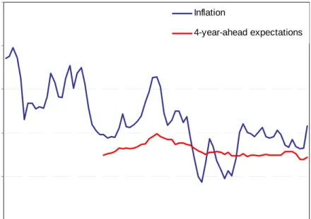
use this sample for two main reasons. The first is that it seems reasonable to assume that inflation
in Mexico followed a stationary process during this period (Figure 1).6 The second reason is that
the Mexican government has been able to issue fixed-rate bonds for long horizons (10 years)
since 2001.7
3
Jeanneau and Tovar (2008) show that among Latin American countries, only Mexico issued bonds with maturities above 20 years in 2007.
4
Chiquiar et al. (2007) find that inflation in Mexico seems to have switched from a non-stationary process to a stationary one around the end of 2000 or the beginning of 2001.
5
We use data of zero-coupon bond yields corresponding to bonds published by Valmer, a firm that provides daily prices for the valuation of financial instruments and other services for analysis and risk management.
6
We conducted Bai and Perron’s (1998) test for structural changes in inflation, and we did not find any change in mean or in trend after 2001.
7
2 3 4 5 6 7 Ju l-0 1 Nov -01 Ma r-0 2 Ju l-0 2 Nov -02 Ma r-0 3 Ju l-0 3 Nov -03 Ma r-0 4 Ju l-0 4 Nov -04 Ma r-0 5 Ju l-0 5 Nov -05 Ma r-0 6 Ju l-0 6 Nov -06 Ma r-0 7 Ju l-0 7 Nov -07 Ma r-0 8 Inflation 4-year-ahead expectations
Figure 1: Inflation and Inflation Expectations. Source: Banco de México.
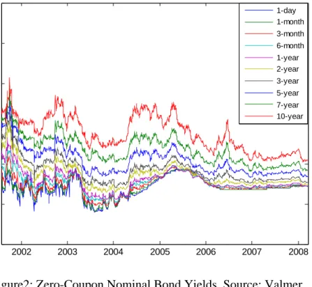
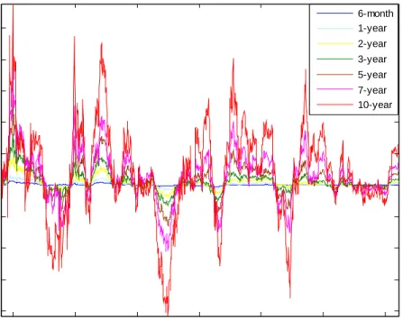
Figure 2 plots the zero-coupon bond yields over the sample period considered. The overall level of zero-coupon bond yields decreased over the sample. In addition, since long-term yields decreased more than short-term yields, the slope of the yield curve also decreased. Long-term yields have declined most likely as the result of the reduction in long-term inflation expectations (Figure 1) and risk premia during the sample period.
Figure 3 plots the average yield curve over the whole sample together with approximate 95% confidence bounds (two times Newey and West’s (1987) standard errors). Yields of bonds with longer maturities were on average higher than those of bonds with shorter maturities. Hence, the yield curve was on average upward sloping. Since the yield curve contains information about market expectations of future short-term interest rates and about risk premia, if the yield curve is upward sloping either people expect interest rates to rise in the future or there are risk premia in long term bonds. The fact that interest rates did not rise on average over the sample suggests the presence of risk premia on long-term bonds (we pursue this further in Section 3).
2002 2003 2004 2005 2006 2007 2008 0 5 10 15 20 25 30 pe rc en t 1-day 1-month 3-month 6-month 1-year 2-year 3-year 5-year 7-year 10-year
Figure2: Zero-Coupon Nominal Bond Yields. Source: Valmer.
0 20 40 60 80 100 120 6 7 8 9 10 11 12 13 14 15 pe rc en t
maturity (in months)
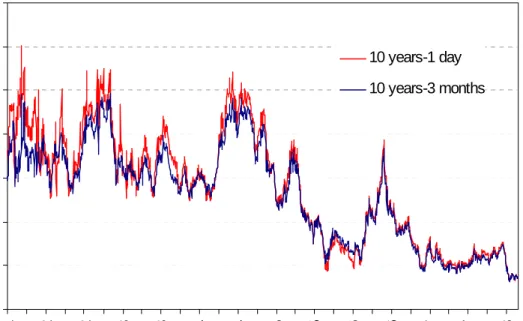
The slope of the yield curve over the whole sample, as proxied by the difference between the 10-year yield and the 1-day yield, or the difference between the 10-10-year yield and the 3-month yield,
has decreased over the sample.8 As can be seen in Figure 4, the low frequency movements show
a gradual reduction in the slope of the yield curve which may be explained by a reduction in inflation and inflation expectations over the sample. As explained below, the high frequency movements result mainly from variations in risk premia and in expected future short-term interest rates. 200 400 600 800 1000 1200 1400 1600 Ju l-0 1 Oc t-0 1 Ja n -0 2 A p r-02 Ju l-0 2 Oc t-0 2 Ja n -0 3 Ap r-0 3 Ju l-0 3 Oc t-03 J a n-04 Ap r-0 4 Ju l-0 4 Oc t-0 4 Ja n -0 5 A p r-05 Ju l-0 5 Oc t-05 Ja n -0 6 Ap r-0 6 Ju l-0 6 Oc t-06 J a n-07 A p r-07 Ju l-0 7 Oc t-0 7 Ja n -0 8 10 years-1 day 10 years-3 months
Figure 4: Yield Curve Slope (Basis Points).
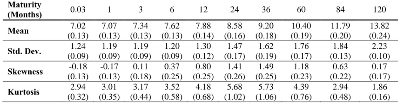
Table I presents some descriptive statistics. This evidence shows that our data are characterized by some standard stylized facts. The average yield curve is on average upward sloping, since average yields increase with maturity. The standard deviations of yields present a u-shape pattern. The yield levels show mild excess kurtosis at medium-term maturities, and positive skewness at medium and long-term maturities.
8
Table I: Descriptive Statistics. Maturity (Months) 0.03 1 3 6 12 24 36 60 84 120 Mean 7.02 (0.13) 7.07 (0.13) 7.34 (0.13) 7.62 (0.13) 7.88 (0.14) 8.58 (0.16) 9.20 (0.18) 10.40 (0.19) 11.79 (0.20) 13.82 (0.24) Std. Dev. 1.24 (0.09) 1.19 (0.09) 1.19 (0.09) 1.20 (0.09) 1.30 (0.12) 1.47 (0.17) 1.62 (0.19) 1.76 (0.17) 1.84 (0.13) 2.23 (0.10) Skewness -0.18 (0.13) -0.17 (0.13) 0.11 (0.18) 0.37 (0.25) 0.80 (0.25) 1.41 (0.26) 1.49 (0.25) 1.18 (0.23) 0.63 (0.22) 0.17 (0.17) Kurtosis 2.94 (0.32) 3.01 (0.35) 3.17 (0.44) 3.52 (0.58) 4.18 (0.68) 5.68 (1.02) 5.73 (1.06) 4.39 (0.76) 2.94 (0.48) 1.86 (0.16)
3.- Time-Varying Risk Premia
To provide evidence of time variation in bond market risk premia, we examine excess holding-period returns for bonds of various maturities in the spirit of Campbell (1995). Variation in excess returns suggests the presence of time-varying risk premia in government bonds. The expectations hypothesis, that long yields are the average of expected future short yields plus a constant term premium, implies that excess returns should be constant. We use historical yield series to answer two questions related to this hypothesis. First, have bonds of different maturities provided equivalent returns for a given holding period? Second, were the returns earned from holding longer-term instruments riskier than they were for shorter-term bonds?
Holding-period returns are calculated for a holding period of 91 days and using zero-coupon instruments with maturities of 0.5, 1, 2, 3, 5, 7 and 10 years. To calculate excess returns, these returns are compared with the yield on a zero-coupon instrument with a 91-day maturity. Excess returns were very volatile during the sample period (Figure 5). For example, investors that sold long-term bonds in June 2006 suffered substantial capital losses (negative excess returns), while investors that sold long-term bonds in September 2006 had capital gains (positive excess returns). Table II shows the summary results for the sample period. It is immediately evident that excess returns get both larger and more volatile as the maturity of the bonds held increases. The results conform with the notion of longer-term assets being riskier, and therefore demanding a positive risk premium. It appears that longer-dated assets carry a positive risk premium to
compensate for the additional volatility of their returns.9
9
Holding period returns were also calculated for holding periods of 30, 60, 180 and 360 days. We found similar results for these holding periods.
2002 2003 2004 2005 2006 2007 2008 -40 -30 -20 -10 0 10 20 30 40 50 pe rc en t 6-month 1-year 2-year 3-year 5-year 7-year 10-year
Figure 5: Excess Holding-Period Returns.
The excess returns support two main conclusions: The term-premia are time-varying, and the expected risk and the expected return increase as the time to maturity of the bond examined increases. These results imply that, to provide an adequate characterization of the Mexican term-structure of interest rates, one should consider models that allow for time-varying risk premia.
Table II: Excess Holding-Period Returns.
Maturity (years) 0.5 1 2 3 5 7 10 Mean 0.16 (0.03) 0.26 (0.08) 0.70 (0.20) 1.17 (0.33) 2.06 (0.57) 2.94 (0.85) 4.18 (1.57) Std. dev. 0.30 (0.03) 0.75 (0.07) 1.84 (0.21) 3.02 (0.33) 5.29 (0.51) 7.97 (0.66) 14.74 (1.14) Skewness 1.58 (0.28) 0.88 (0.22) 1.14 (0.31) 1.02 (0.32) 0.58 (0.31) 0.05 (0.27) -0.24 (0.21) Kurtosis 5.77 (1.38) 4.41 (0.80) 5.76 (1.15) 5.64 (1.09) 4.61 (0.73) 3.85 (0.48) 3.48 (0.37)
4.- Principal-Components Analysis
In this section, we use principal components analysis, as proposed by LS, to describe the
behavior of the yield curve over time.10 This approach has at least two advantages: it allows us to
summarize all the information contained in the yield curve using a small number of factors, and it delivers some intuition for what drives the dynamics of zero-coupon bond yields. Since the seminal work of LS, several authors have recognized the importance of identifying the common factors that affect the term-structure of interest rates. To explain the variation in these rates, it is critical to distinguish the systematic risks that have a general impact on the yield curve from the specific risks that influence individual bonds. Principal components can be computed from levels
and changes in yields, so we will do both.11
Looking at the estimated principal components reveals that much of the variance in yields is explained by the first principal component. Table III computes the cumulative percentage in the variation of yields changes and levels explained by the principal components. The table shows that the first 3 principal components already explain over 99% of the total variation in yields. In the case of yield changes, the first 3 principal components explain over 85% of their total variation. These results indicate that, similar to LS's results for the US, 99% of the variation in the Mexican zero-coupon yield curve can be explained in terms of only three uncorrelated factors. These can be interpreted as there being three major sources of aggregate risk driving the dynamics of the term-structure in Mexico, a result similar to what has been found for developed economies.
Table III: Variation in Yield Changes and Levels.
P.C. 1 2 3 4 5 6 7 8 9 10
% explained in
Yt 78.56 95.01 99.31 99.64 99.77 99.87 99.92 99.96 99.99 100
% explained in
∆Yt 53.49 75.61 85.45 91.89 94.61 96.65 97.75 98.77 99.45 100
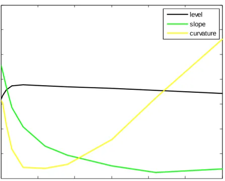
We refer to the sensitivity of a bond's yield to a common factor as the loading of the bond yield on that factor. Figure 6 plots the components of the eigenvectors corresponding to the first three factors, as a function of the maturity of the yields in months. The loadings of the first principal component are almost horizontal. This pattern means that changes in the first principal component correspond to parallel shifts in the yield curve. This principal component is therefore called the level factor. The loadings of the second principal component are downward sloping. Changes in the second principal component thus rotate the yield curve. This means that the second component is a slope factor. A positive change in this component will induce a rise of the short-end of the yield curve, and a fall of the long-end of the curve. This slope factor will cause the yield curve to flatten (positive change), or to steepen (negative change). The third principal component corresponds to the curvature factor, because it causes the short and long ends to increase, while decreasing medium-term yields. The third principal component therefore affects
10
On principal components, see Izenman (2008). 11
Alemán and Treviño (2006) also use principal components on data from the yield curve in Mexico, although for a shorter sample.
the curvature of the yield curve. The loadings of the principal components of yield changes look similar. 0 20 40 60 80 100 120 -0.4 -0.2 0 0.2 0.4 0.6 0.8 1 maturity in months level slope curvature
Figure 6: Loadings of Yields on Principal Components.
The interpretation of these principal components in terms of level, slope and curvature goes back to LS. These labels have turned out to be extremely useful in thinking about the driving forces of the yield curve. The latent factors implied by estimated affine models typically behave like the factors obtained through principal components (Ang and Piazzesi, 2003).
Traditional factor models provide a natural benchmark for the cross-sectional fit. Factor models
based on a few principal components can predict all n yields in the cross-section. The difference
between actual yields and model-predicted yields are defined as fitting errors. Table IV computes the mean, standard deviation and maximum of the absolute value of these fitting errors using the first three principal components. The absolute fitting errors are less than 13 basis points for all yields in the data. This means that this low-dimensional factor model not only explains much of the variance in yields, but also performs extremely well according to this additional metric.
Table IV: Absolute Value of Fitting Errors for Yields.
Maturity
(months) 0.03 1 3 6 12 24 36 60 84 120
Mean 0.13 0.07 0.08 0.10 0.10 0.07 0.07 0.09 0.11 0.06
Std. Dev. 0.15 0.08 0.10 0.10 0.09 0.07 0.06 0.09 0.08 0.05
5.- Term-Structure and Macroeconomic Dynamics
Since most of the variation of the yield curve in Mexico is explained by the first two principal components (95%), we concentrate on the dynamics of these two components. It is possible to construct a time series for these using the information in the matrix of eigenvectors and the zero-coupon bond yields. This allows the comparison of these components with standard empirical proxies for level and slope.
Since the principal components are linear combinations of all yields, and the coefficients are the eigenvectors of the variance-covariance matrix of the zero-coupon bond yields, we can calculate the paths of all the principal components over time using the columns of the matrix of eigenvectors. The first two principal components in our model correspond to empirical proxies for the level and slope of the yield curve, respectively. In particular, the first principal component and a common empirical proxy for the level (namely, the average of the 1-day, 1-year and 10-year yields) have a correlation of 0.97. This supports our interpretation of the first principal component as a level factor. The second principal component and a standard empirical slope proxy (the 10-year minus the 1-day yield) have a correlation of 0.75. This lends credibility to our
interpretation of the second principal component as a slope factor.12
Some interesting facts are worth mentioning. First, both the first principal component and the level of the yield curve fell sharply during the sample period. Second, both the slope of the yield curve and the second principal component also fell during the sample period, indicating a flattening of the yield curve over the sample period.
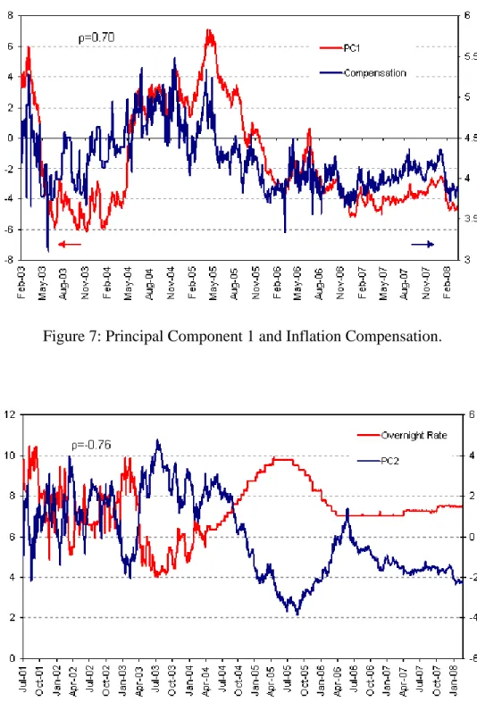
The level of the yield curve has been associated in the term-structure literature with measures of long-term inflation expectations. For example, Rudebusch and Wu (2003) interpret the difference between nominal and inflation-linked yields as a measure of expected inflation. Figure
7 displays the first principal component and a measure of long-run inflation compensation.13 The
correlation between this component and long-run inflation compensation, which is 0.70, is consistent with a link between the level of the yield curve and inflationary expectations, as suggested by the Fisher equation. This link is a common theme in the recent macro-finance
literature, including Dewachter and Lyrio (2006), and Hördahl et al. (2006).
The term-structure literature has also shown that the yield curve slope is connected to the cyclical dynamics of the economy (Piazzesi 2005). The overnight interest rate is the instrument under control of the central bank, that adjusts in response to macro shocks in order to achieve the economic stabilization goals of monetary policy. Therefore, the slope of the yield curve should be related to the policy rate. Figure 8 provides some evidence about the relationship between the slope of the yield curve and the overnight interest rate. The correlation between the second principal component and the overnight rate, which is -0.76, suggests that the yield curve slope is related to the cyclical response of the central bank. This evidence suggests that shocks that induce the central bank to move the short-term interest rate move the slope of the yield curve in the opposite direction. This evidence is consistent with Ang and Piazzesi (2003) and Rudebusch
12
Ang and Piazzesi (2003) and Diebold et al. (2006), among others, have used these proxies. 13
We measure inflation compensation as the spread between 10-year yields on nominal and indexed securities. Inflation compensation contains both, inflation expectations and the inflation premium.
and Wu (2003), who find that in the US the short-term interest rate and the slope factor are negatively correlated.
Figure 7: Principal Component 1 and Inflation Compensation.
6.- Conclusions
Little is known about the behavior of the term structure of interest rates in emerging markets. We have analyzed its behavior in one such market, that for Mexican government bonds. Three conclusions can be drawn from this analysis. First, we find that term-premia in the Mexican government bond market appear to be time-varying. Second, we show that, similar to bond markets in advanced economies, over 99% of the total variation in the yield curve can be explained by three factors. The first factor captures movements in the level of the yield curve, the second captures movements in the slope of the curve, and the third one captures its curvature. Third, we find that the level factor is positively correlated with measures of long-term inflation expectations and that the slope factor is negatively correlated with the overnight interest rate (the monetary policy instrument). Hence, the term structure of interest rates in Mexico seems to behave as in markets that have more developed financial systems and that have enjoyed macroeconomic stability, in particular low and stable inflation, for much longer.
Our finding that, as in developed economies, the term structure in a stable emerging economy can be summarized with only a few factors suggests that it may have a similar behavior in other important emerging markets. Our finding may have been expected given the success of this framework in developed countries, and given that if a country is able to issue medium and long-term bonds for a number of years may be because it is already performing as a developed country in this respect (e.g., fiscal discipline, central bank independence). However, the fact that the statistical factors appear to be the same in advanced and in stable emerging economies does not imply that the economic forces behind the statistical factors are the same. In current research, we are analyzing this important issue for the Mexican case.
References
Alemán, J., and J. Treviño (2006) “Monetary policy in Mexico: A yield curve analysis approach” Mimeo, Banco de México.
Ang, A. and M. Piazzesi (2003) “A no-arbitrage vector autoregression of term structure
dynamics with macroeconomic and latent variables” Journal of Monetary Economics50, 745-87.
Bai, J. and P. Perron (1998) “Estimating and testing linear models with multiple structural
changes” Econometrica66, 47-78.
Borensztein, E., K. Cowan, B. Eichengreen and H. Panizza (Eds.) (2008) Bond Markets in Latin
America, The MIT Press: Cambridge.
Capistrán, C. and M. Ramos-Francia (2009) “Inflation dynamics in Latin America” Contemporary Economic Policy27, 349-62.
Campbell, J. (1995) “Some lessons from the yield curve” The Journal of Economic Perspectives
Chiquiar, D., A.E. Noriega and M. Ramos-Francia (2007) “A time series approach to test a change in inflation persistence: The Mexican experience” Banco de México working paper series
2007-1. Forthcoming in Applied Economics.
DeWachter, H. and M. Lyrio (2006) “Macro factors and the term structure of interest rates” Journal of Money, Credit and Banking38, 119-40.
Diebold, F.X., M. Piazzesi and G.D. Rudebusch (2005) “Modeling bond yields in finance and
macroeconomics” American Economic Review P&P95, 415-20.
Diebold, F.X., G.D. Rudebusch and S.B. Aruoba (2006) “The macroeconomy and the yield
curve: A dynamic latent factor approach” Journal of Econometrics131, 309-38.
Evans, C.L. and D. Marshall, (1998) “Monetary policy and the term structure of nominal interest
rates: evidence and theory” Carnegie-Rochester Conference Series on Public Policy49, 53-111.
Hördahl, P. O. Tristani, and D. Vestin (2006) “A joint econometric model of macroeconomic and
term structure dynamics” Journal of Econometrics131, 405-44.
Izenman, A.J. (2008) Modern Multivariate Statistical Techniques, Springer: New York.
Jeanneau, S., and C. Tovar (2008) “Domestic bond markets in Latin America: Achievements and
challenges” BIS Quarterly ReviewJune, 51-64.
Litterman, R. and J. Scheinkman (1991) “Common factors affecting bond returns” Journal of
Fixed Income1, 54-61.
Newey, W.K. and K.D. West (1987) “A simple, positive semi-definite, heteroskedasticity and
autocorrelation consistent covariance matrix” Econometrica55, 703-08.
Piazzesi, M. (2005) “Bond yields and the Federal Reserve” Journal of Political Economy 113,
311-44.
Rudebusch, G.D. and T. Wu (2003) “A macro-finance model of the term structure, monetary policy, and the economy” Manuscript, Federal Reserve Bank of San Francisco.
Sargent T.J. and N. Wallace (1981) “Some unpleasant monetarist arithmetic” Federal Reserve