NBER WORKING PAPER SERIES
CURRENCY CHOICE AND EXCHANGE RATE PASS-THROUGH Gita Gopinath
Oleg Itskhoki Roberto Rigobon Working Paper 13432
http://www.nber.org/papers/w13432
NATIONAL BUREAU OF ECONOMIC RESEARCH 1050 Massachusetts Avenue
Cambridge, MA 02138 September 2007
We wish to thank the international price program of the Bureau of Labor Statistics for access to unpublished micro data. We owe a huge debt of gratitude to our project coordinator Rozi Ulics for her invaluable help on this project. The views expressed here do not necessarily reflect the views of the BLS. We thank Mark Aguiar, Pol Antras, Ariel Burstein, Linda Goldberg, Emi Nakamura, Andy Neumeyer, Ken Rogoff, Daryl Slusher and seminar participants at numerous venues for their comments. We thank Igor Barenboim, Loukas Karabarbounis and Kelly Shue for excellent research assistance. A previous version of this paper was circulated under the title ''Pass-through at the Dock: Pricing to Currency and to Market?'' This research is supported by NSF grant #SES 0617256. The views expressed herein are those of the author(s) and do not necessarily reflect the views of the National Bureau of Economic Research.
© 2007 by Gita Gopinath, Oleg Itskhoki, and Roberto Rigobon. All rights reserved. Short sections of text, not to exceed two paragraphs, may be quoted without explicit permission provided that full credit, including © notice, is given to the source.
Currency Choice and Exchange Rate Pass-through Gita Gopinath, Oleg Itskhoki, and Roberto Rigobon NBER Working Paper No. 13432
September 2007 JEL No. E31,F3,F41
ABSTRACT
A central assumption of open economy macro models with nominal rigidities relates to the currency in which goods are priced, whether there is so-called producer currency pricing or local currency pricing. This has important implications for exchange rate pass-through and optimal exchange rate policy. We show, using novel transaction level information on currency and prices for U.S. imports, that even conditional on a price change, there is a large difference in the pass-through of the average good priced in dollars (25%) versus non-dollars (95%). This finding is contrary to the assumption in a large class of models that the currency of pricing is exogenous and is evidence of an important selection effect that results from endogenous currency choice. We describe a model of optimal currency choice in an environment of staggered price setting and show that the empirical evidence strongly supports the model's predictions of the relation between currency choice and pass-through. We further document evidence of significant real rigidities, with the pass-through of dollar pricers increasing above 50% in the long-run. Lastly, we numerically illustrate the currency choice decision in both a Calvo and a menu-cost model with variable mark-ups and imported intermediate inputs and evaluate the ability of these models to match pass-through patterns documented in the data.
Gita Gopinath Department of Economics Harvard University 1875 Cambridge Street Littauer Center Cambridge, MA 02138 and NBER gopinath@harvard.edu Oleg Itskhoki Department of Economics Harvard University 1875 Cambridge Street Cambridge, MA 02138 itskhoki@fas.harvard.edu Roberto Rigobon
Sloan School of Management MIT, Room E52-431
50 Memorial Drive
Cambridge, MA 02142-1347 and NBER
1
Introduction
In the open economy macro literature with nominal rigidities, the currency in which goods are priced has important implications for the pass-through of exchange rates into traded goods prices and for optimal exchange rate policy. In a large class of models, the currency of pricing is exogenous. That is, prices are exogenously set either in the producer currency or in the local currency.1 In such models, the difference in pass-through is a short-run phenomenon. In the short run, when prices are rigid, pass-through into import prices of goods priced in the producer’s currency is 100% and it is 0% for goods priced in the local currency. However, when prices adjust, there is no difference in pass-through.
We show, using novel transaction level information on currency and prices for U.S. im-ports, that even conditional on a price change, there is a large difference in the pass-through of the average good priced in dollars (25%) versus non-dollars (95%). This finding is contrary to the assumption of a large literature that assumes the currency of pricing is exogenous. It is evidence of an important selection effect and is consistent with a separate literature on endogenous currency choice recently reviewed in Engel (2006). In this environment, the dif-ference in pass-through between producer currency pricing (PCP) and local currency pricing (LCP) firms persists even conditional on adjusting prices. Evidence of this selection effect reduces the importance of the direct effect of nominal rigidities in explaining differences in pass-through across the different pricing regimes.
Given the observed strong relationship between currency of pricing and measured pass-through at different horizons, we explore both theoretically and empirically the relation between currency choice and pass-through in this paper. The paper is structured as follows. To motivate our analysis, we first show, in Section2, using aggregate price index regressions that the difference in pass-through into U.S. import prices of the average good priced in dollars versus the average good priced in non-dollars is large at horizons starting from 1 month all the way out to 24 months. The pass-through into dollar (non-dollar) priced goods is close to 0 (1) in the short-run and is 0.14 (0.92) at 24 months. The difference therefore declines from 1 in the short-run to around 0.75 at 24 months. Such sizeable and significant differences are shown to hold for individual countries exporting to the U.S. across dollar and non-dollar goods. The feature that short-run pass-through is dramatically different, when prices have not adjusted, is consistent with currency choice being exogenous or endogenous. However, the finding that even at horizons of 24 months this difference persists is evidence of an important selection effect that arises when currency choice is endogenous.
1For instance, Obstfeld and Rogoff (1995) assume producer currency pricing, Betts and Devereux (2000) and Chari, Kehoe, and McGrattan (2002) assume local currency pricing. Devereux and Engel (2003) allow prices to be exogenously set both in local and producer currencies.
Next, we describe in Section 3, a model of optimal currency choice in an environment of staggered price setting. There exists a large literature on optimal currency choice as surveyed in Engel (2006)2 who also presented an important equivalence result between optimal pass-through and the optimal currency of pricing.3 However, the analysis in the literature has been conducted in a static environment where prices are pre-set only one period in advance. We consider here a dynamic multi-period staggered price setting model. In this environment, we make a distinction between optimal pass-through when the firm adjusts its price but all other firms have not adjusted and the optimal long-run (or flexible price) pass-through when all firms have fully adjusted their prices. Currency choice is shown to depend on the pass-through conditional on the first instance of price adjustment to the exchange rate shock. We refer to this as themedium-runpass-through and it is determined by both the dynamic path of desired pass-through and the duration of non-adjustment. Currency choice cannot be predicted solely by long-run pass-through or desired pass-through on impact of the exchange rate shock. This result does not depend on the specific source of incomplete pass-through, that is if it is variable mark-ups, imported inputs, decreasing returns to scale in production, etc. If real rigidities in the pricing decisions of firms are important, medium-run pass-through can differ from long-run pass-through. Specifically, a firm with a high flexible price (long-run) pass-through can well choose local currency pricing if real rigidities lead to a low desired pass-through in the short-run.
We then use the model to derive pricing equations that can be used to estimate the pass-through coefficients that affect the currency choice decision. Previous empirical work on currency choice has been limited by the lack of sufficiently disaggregated data on prices and currency of denomination. As Engel (2006) pointed out, without detailed price data, it is hard to disentangle the effect of nominal from real rigidities on exchange rate pass-through. We remedy this by using unpublished micro-data on firm level import prices collected by the Bureau of Labor Statistics for the U.S., for the period 1994-2005. There are several reasons why this data is particularly suited to our analysis. Firstly, there is reported transaction level currency information which is unique to this database. Secondly, we observe the individual goods price series and therefore can condition our analysis on the instances when prices change, which is required to estimate a theoretically appropriate measure of pass-through
2The papers in this literature include Giovannini (1988); Friberg (1998); Bacchetta and van Wincoop (2003, 2005); Devereux, Engel, and Storgaard (2004); Corsetti and Pesenti (2004); Goldberg and Tille (2005).
3The intuition for this result is as follows: Currency choice is essentially a zero-one indexing decision of firm’s price to exchange rate shocks. If prices adjust every period, currency choice is irrelevant. However when prices are sticky, the firm can use currency choice to make its price closer to the desired price in periods when the firm does not adjust it. Producer (local) currency pricing assures 100% (0%) pass-through in the short run, prior to price adjustment. Therefore, the higher is the desired pass-through in the short-run, the higher are the gains from pricing in producer currency compared to local currency.
for currency choice.
The empirical analysis in Section 4provides strong support for the theoretical mapping between currency choice and medium-run exchange rate pass-through. We show that condi-tioning on a price change, the elasticity of response of prices to the cumulative exchange rate change over the period of non-adjustment is only 25% for dollar pricers as compared to 95% for non-dollar pricers. Secondly, we find evidence of significant real rigidities for dollar priced goods that mutes the initial response of firms’ prices to exchange rate shocks. We find that exchange rate shocks that took place prior to the most recent period of non-adjustment have strong and significant effects on current price adjustments. As a result, the pass-through of dollar pricers increases to above 50% in the long-run. The difference in pass-through between dollar and non-dollar priced goods in the long-run comes down to 42% as opposed to 70% conditional on the first price adjustment. The finding that long-run pass-through for some dollar pricers can be as high as 60% is consistent with the fact that what matters for currency choice is the medium-run pass-through and not the long-run pass-through.
The empirical results are not specific to a particular model of incomplete pass-through and stand on their own as facts that need to be matched by models of exchange rate pass-through. In the final section, Section 5, we consider a model with two sources of incomplete long-run pass-through — variable mark-ups arising from Kimball demand preferences and imported inputs in production. We numerically analyze the behavior of a Calvo and a Menu-cost models of price setting with these features. We show that a firm is more likely to select into producer currency pricing the lower the elasticity of its mark-up and the lower the share of imported inputs in its production cost. For reasonable parameter values we find that the model can generate low long-run import pass-through as in the data. In both models, desired pass-through has an increasing profile which translates into a lower medium-run pass-through as compared to the long-run pass-through. However, in the menu cost model the size of this difference is small: a firm adjusting on the day of the shock will pass-through 90% of what is optimal in the long run; a firm adjusting 6 months after the shock will already decide to pass-through the optimal long-run amount. In the Calvo model, the results are quantitatively different. The medium-run pass-through is about 70% of that in the long-run which is closer to the empirical estimate of 50% and the long-run is achieved only after several rounds of price adjustments.
Data
We use unpublished micro data on import prices collected by the Bureau of Labor Statistics for the period 1994-2005. This data are collected on a monthly basis and have information on import prices of a very detailed good over time, with details on the country of origin and the currency of pricing. Details regarding the underlying database are reported in Gopinath and Rigobon (2007).
In the price survey, the BLS asks firms to report on the currency of denomination of the price. Gopinath and Rigobon (2007) document that prices are rigid, with a median duration of 11 months, in the currency in which they are reported as being priced in.4 Around 90% of U.S. imports in the BLS sample are reported as priced in dollars. This fraction however varies by country of origin. The fraction of imports in the exporters currency is, for example, 34% from Germany, 16% from U.K. and 13% from Japan. From all developing countries the share in the exporters currency is close to zero. As is well known, a significant fraction of trade takes place intra-firm. This database allows us to identify transactions as taking place intra-firm or at arms-length. Since we will test theories of prices that are driven mainly by market forces we exclude intra-firm prices from our analysis.5
In our empirical analysis we include countries that have a non-negligible share of their exports to the U.S. priced in both dollar and non-dollar currency. This includes Germany, Switzerland, Italy, Japan, UK, Belgium, France, Sweden, Spain, Austria, Netherlands and Canada.6 In Table 1 we present the number of goods, country by country, that are invoiced in dollars (first column), in the exporter’s currency (second column), and the fraction of goods that are invoiced in the exporter’s currency (last column).
2
Aggregate ERPT and Currency of Pricing
To motivate our analysis we present estimates of exchange rate pass-through across dollar and non-dollar priced goods using aggregated price indices that we construct from the underlying data. We show that the difference in pass-through into U.S. import prices of the average good priced in dollars versus the average good priced in non-dollars is large even at horizons
4This fact suggests that the currency information is meaningful and it is not the case, for instance, that firms price in non-dollars and simply convert the prices into dollars to report to the BLS. For this would imply that dollar prices would then show a high frequency of adjustment, which is not the case.
5For empirical evidence on the differences between intra-firm and arms-length transactions, using this data, see Gopinath and Rigobon (2007) and Neiman (2007).
6We used the following two formal criteria for selection: (1) a country should have at least 10 items priced in non-dollars; and (2) at least 5% of all items imported from a country should be priced in non-dollars.
longer than a year.
For each country we construct two separate price indices – one including only goods that are priced in dollars and the other using only those goods priced in the exporter’s currency. For most countries, for exports to the U.S., these are the only two types of pricing.7 Some goods are priced in a third currency, but such instances are rare. The index we construct is un-weighted, since we were not provided with BLS weights at the good level for the whole period.
We estimate the following standard pass-through specification, ∆pi,t =α+ n X j=0 β1,j∆ei,t−j + n X j=0 β2,jπi,t−j+ 3 X j=0 β3,j∆yt−j+²t (1)
wherei indexes the country, ∆p is the monthly change in the price index in dollars,π is the monthly foreign country inflation using the producer price index, and ∆y is average GDP growth in the U.S.; n is the number of lags which varies from 1 to 24. Since the data is monthly, we include up to 24 lags for the nominal exchange rate and foreign inflation and 3 lags for GDP growth.8
The statistic of interest is the sum of the coefficients on the nominal exchange rate:
β(n) ≡ Pnj=0β1,j. These coefficients reflect the impact that the current change in the exchange rate has on the price index of imports over time. The objective is to compare these estimates across different currency indices as we increase the number of lags included in the specification from 1 to 24. Figure 1 depicts the pass-through coefficients from estimating a pooled regression of all countries with the number of lags on the x-axis. The line in the middle depicts the pass-through for the aggregate index. This measure of pass-through increases from 0.22 with one lag to 0.30 with 24 lags. The feature that at the aggregate level most of the pass-through takes place in the first two quarters and levels off soon after is consistent with the findings of Campa and Goldberg (2005) and others who have estimated pass-through into the U.S. using the BLS price index.
From just this aggregate index, however, it is impossible to discern the role of currency. Now we consider the separate currency indices. The top line depicts the pass-through for the non-dollar index. The bottom line is the pass-through for the dollar invoiced index. The bands represent the 95% confidence interval around the point estimate for each lag specification. As Figure 1demonstrates, the regression using only the contemporaneous and
7Some non-dollar items keep their dollar price fixed for a few months and then index to the cumulative exchange rate change. However, these cases are few in number. We have excluded such hybrid cases from our specification, however they had little influence on the results.
8We have also estimated similar equations including controls for U.S. inflation and find that the results are insensitive to this.
1 4 8 12 16 20 24 0 0.2 0.4 0.6 0.8 1 Horizon, months Non−Dollar Dollar Aggregate
Figure 1: Aggregate ERPT at different horizons by currency
1 month lag of the exchange rate estimates a pass-through of 0.03 for goods priced in dollars and 0.96 for goods priced in non-dollars. Further, we observe that the pass-through increases for the dollar items with the inclusion of lags, while it decreases slightly for the non-dollar index. This is consistent with the pattern of price stickiness documented in the data. Note that the pass-through into the dollar priced goods is far more gradual than is suggested by the pass-through into the aggregate index. A striking feature of the plot is that the gap between pass-through of the dollar and non-dollar index remains large and significant even 24 months out. At 24 months the pass-through is 0.30, 0.14 and 0.94 respectively for the aggregate, dollar and non-dollar indices.
In Figure 2, we replicate the aggregate regressions country by country. Notice that the aggregate level of pass-through varies substantially across countries. This can be seen from the middle line in the plots. For instance, for Germany, the pass-through is 40 percent in the short run and increases slightly to 45 percent when 24 lags are included. For Japan and Italy, the numbers are smaller, as they increase from below 25 percent to 30 percent, while for Sweden and France pass-through is always smaller than 20 percent. The difference between the pass-through of the dollar and non-dollar index is again quite striking. The exception to this is Canada where the two through elasticities intersect. Average pass-through for Canada increases from 20 percent in the short run to almost 60 percent in 24 months, though these numbers are highly imprecisely estimated. For all other countries
1 8 16 24 Germany 1 8 16 24 United Kingdom 1 8 16 24 France 1 8 16 24 0 0.25 0.5 0.75 1 Italy 1 8 16 24 0 0.25 0.5 0.75 1 Switzerland 1 8 16 24 Japan 1 8 16 24 Sweden 1 8 16 24 Spain 1 8 16 24 0 0.2 0.5 0.75 1 The Netherlands 1 8 16 24 Austria 1 8 16 24 Canada
Figure 2: Aggregate ERPT at different horizons by currency from specific countries
the differences remain large even at long horizons and for 9 out of the 12 countries the difference is significant even for the specification with 24 lags. The two exceptions, other than Canada, are Austria, and Netherlands for which there is simply not enough data to statistically distinguish the two pass-through elasticities at 24 months horizon. Notice that
in all other countries the confidence intervals for the dollar and non-dollar pass-through do not intersect.
It is important to emphasize that the average pass-through numbers we obtain (the middle line) are very close to the numbers estimated using the publicly available BLS price index. For imports from Japan and Canada the BLS reports a price index starting from 1994. We find that the measure of aggregate pass-through using our index is very close to the numbers using the BLS price index. Specifically, using the BLS index, the estimate for Canada is 57 percent, and it is 31 percent for Japan, while we obtain a pass-through of 0.60 and 0.29 respectively. What we do additionally is to decompose that index by currency of pricing and we find that the pass-through elasticities at long horizons are very different for these two sub-indices.
0 0.1 0.2 0.3 0.4 0.5 0 0.1 0.2 0.3 0.4 0.5 0.6 Fraction of PCP firms Aggregate ERPT
Figure 3: Fraction of PCP firms and Aggregate ERPT
Another striking feature of Figure 2 is how similar pass-through patterns are across the countries once we condition on currency choice, despite the cross-country differences in aggregate pass-through coefficients. In other words, given the large and persistent differences in pass-through related to the currency of invoicing, the fraction of goods that are priced in different currencies, should have significant prediction power for the measures of aggregate import pass-through, even at very distant horizons. We illustrate this point in Figure 3. Each dot in this figure represents a country and its coordinates are the fraction of ‘non-dollar firms’ importing from this country on the x-axis and the aggregate ERPT from this country on the y-axis. The line in the figure is not a regression, but simply a line which connects 0.14 ERPT (which is the average pass-through for LCP firms) when the fraction of PCP firms is 0 and 0.94 (which is the average pass-through for PCP firms) when this fraction is 1. The only outlier in this figure is Canada and the correlation between the two plotted variables is 0.87 excluding Canada.
The results in this section demonstrate that unlike the models that assume exogenous currency choice, exchange rate pass-through of PCP and LCP firms do not equalize even after most prices have had enough time to adjust. This is evidence of the endogeneity of currency choice and the significance of this selection effect. This motivates our analysis in the following sections.
We proceed in the following steps. First, we present a general result on the relation between currency choice and medium-run pass-through in an environment of staggered price setting in Section3.1. We do this without specifying the source of incomplete pass-through, that is if it is variable mark-ups, imported inputs, decreasing returns to scale in production, etc. Then in Section 3.2 we introduce two channels of incomplete pass-through — variable mark-ups and imported inputs. By doing so we demonstrate conditions under which medium-run pass-through, on which currency choice depends, can differ from long-medium-run pass-through. Next, in Section4we empirically test the implications of the model for the relation between currency choice and medium-run pass-through and we also test for the presence of real rigidities. These empirical results stand on their own as facts that need to be matched by models of exchange rate pass-through. Until this point we intentionally abstract from specific models of variable mark-ups and incomplete pass-through, so as to emphasize the generality of the results. In the final section, Section 5, we consider a particular source of variable mark-ups, namely Kimball demand preferences, alongside imported inputs in production to evaluate the ability of a Calvo and a Menu-cost models of price setting to match the facts in the data.
3
Currency Choice in a Dynamic Sticky Price Model
In this section we discuss the optimal currency choice for price setting by firms in an environ-ment with sticky prices, in a partial equilibrium set-up. We allow the firm to choose between local currency (LCP) and producer currency pricing (PCP). There exists a large literature on currency choice in environments with prices set one period in advance. Instead, we consider a multi-period setting and derive new insights which cannot be shown in a one-period model. While there are several important papers in the theoretical literature on currency choice,9 our paper is most closely related to Engel (2006). Engel (2006) showed that in an environ-ment with one-period-ahead price setting, flexible price pass-through is a sufficient statistic for currency choice. Specifically, if the flexible price pass-through is greater than a cer-tain threshold, the firm should choose producer currency pricing which guarantees complete
short-run pass-through, before the firm adjusts its price. On the other hand, if the flexible price pass-through is low, the firm should choose local currency pricing which assures zero pass-through in the short-run.
This section extends the important insight of Engel (2006) and analyzes an environment with an arbitrary amount of price stickiness. We make a distinction between pass-through when the firm adjusts its price but all other firms have not adjusted and the long-run (or flexible price) pass-through when all firms have fully adjusted their prices. In this environ-ment, currency choice depends on the pass-through conditional on the first instance of price adjustment to the exchange rate shock. We refer to this as themedium-run pass-through and it is a function of the dynamic path of desired pass-through and the frequency of adjustment. Medium-run pass-through can differ from the long-run (flexible price) pass-through if real rigidities such as strategic complementarities in the pricing decisions of firms are important. Specifically, a firm with a high long-run pass-through can well choose local currency pricing if strategic complementarities are strong and lead to a low medium-run pass-through.
3.1
Medium-run Pass-through and Currency Choice
We consider here the case of Calvo staggered price setting where a firm who gets to change its price can also choose the currency in which to price.10 The assumption of Calvo price setting allows us to characterize analytically the optimal currency choice rule. In Section 5 we will show numerically that the theoretical insights of this section extend to a model with menu costs and endogenous frequency of price adjustment.11
Consider an exporting firm with a profit function Π¡p;s¢, where pis the local currency price of the firm (in logs) andsis the remaining state vector;scan include the industry price level, demand and cost variables, etc. For now we do not specify what these variables are. This is left to the next subsection. Define ˜p(s) = arg maxpΠ(p;s) to be the static optimal price of the firm in states and denote ˜Π(s)≡Π¡p˜(s);s¢. We will refer to ˜p(s) as the desired price of the firm, i.e. the price that the firm would set if it adjusted every period in the given environment.12
10We show later the conditions under which the currency choice rule would be the same if currency was chosen only once during the life of the good.
11According to the empirical evidence in Gopinath and Rigobon (2007), exchange rate movements do not play a predominant role in explaining the probability of price adjustments. Therefore, the assumption of exogenous frequency of price adjustment is not very restrictive for the purposes of studying optimal currency choice decisions.
12There is a difference between flexible price and desired price. When we sayflexible price, we imply that the firm operates in a flexible price environment which imposes a certain selection criteria on the set of states
sthat can be consistent with the flexible price equilibrium (in particular, since the sectoral price level can be part of the state space). When we say desired price, we refer to the pricing decision of a flexible-price
Denote the history of the states by st = (s
0, . . . , st). The state space can be segmented into st = (et, ht), where et is the log of the exchange rate13 and ht contains the remaining state variables. Further, we assume that the exchange rate follows an exogenous random walk process.14 Nevertheless, state variablesh
t can be correlated with current or past shocks to the exchange rate and can exhibit arbitrary amount of persistence. We assume that the firm discounts the future at a constant rate δ.
Consider a firm that decides to set its current price in the local currency. The Bellman equation for the value of this firm is then
VL ¡ p;st¢= Π¡p;s t ¢ +δθE©VL ¡ p;st+1¢¯¯st, ϑ t+1= 0 ª (2) +δ(1−θ)E©V¯¡st+1¢¯¯st, ϑ t+1= 1 ª ,
where ϑτ is the indicator variable for price adjustment in period τ which equals 0 with probability θ, independently of any exogenous state variable.15 If the firm adjusts in state
st, it sets the price according to ¯p(st) = arg max
pVL(p;st), and we denote by ¯VL(st) ≡
VL
¡
¯
p(st);st¢the value of the firm conditional on price adjustment and local currency pricing. Finally, ¯V(st) is the continuation value defined below which allows for the optimal choice of the currency of pricing.
A similar Bellman equation holds for a firm setting its current price in its own (producer) currency: VP ¡ p∗;st¢= Π¡p∗+e t;st ¢ +δθE©VP ¡ p∗;st+1¢¯¯st, ϑ t+1= 0 ª (3) +δ(1−θ)E©V¯¡st+1¢¯¯st, ϑ t+1= 1 ª ,
where p∗ is the producer currency price of the firm. The optimal price is then ¯p∗(st) = arg maxp∗VP(p∗;st) and again we denote ¯VP(st)≡VP
¡
¯
p∗(st);st¢. The continuation value is then naturally defined as ¯V(st) = max{V¯
L(st),V¯P(st)}.
Before discussing the optimal currency choice, we prove a familiar certainty equivalence result which will be useful for our further analysis:
Proposition 1 Up to the second order, the optimal prices in the local currency for both LCP and PCP firms are equal to the weighted average desired price in all future periods and
firm in a given sticky price environment. As a result, pass-through into flexible prices can be different from pass-through into desired prices if, for example, strategic complementarities are important.
13Exchange rate is defined in the standard way so that an increase in et corresponds to appreciation of the foreign currency.
14All the results can be extended in a natural way to an environment with mean reversion in the exchange rate, however this case is empirically less relevant and we omit it from the text for brevity.
15Note that expectations in (2) must be conditioned on whether the firm adjusts its price since this may affect endogenous state variables such as the intra-industry price level.
states conditional on the preset price remaining effective. Formally, ¯ p(st) = (1−δθ) ∞ X `=0 (δθ)`E©p˜(st+`) ¯ ¯st, ϑ t+1=. . .=ϑt+`= 0 ª (4) and ¯ p∗(st) = (1−δθ) ∞ X `=0 (δθ)`E©p˜∗(st+`) ¯ ¯st, ϑ t+1=. . .=ϑt+`= 0 ª , (5) where p˜∗(s
t+`) = ˜p(st+`)−et+` is the desired price in producer currency. Consequently, up to the second order of approximation, p¯(st) = ¯p∗(st) +e
t. Proof: See Appendix ¥
Proposition 1, despite being standard in the monetary economics literature (e.g., see Dotsey, King, and Wolman (1999)), has an interesting implication in the international con-text when firms are allowed to choose between local and producer currency pricing. Specifi-cally, Proposition 1 shows that two firms pricing in different currencies but similar in all other respects will choose the same prices in local currency, conditional on adjustment.16 There-fore, all the differences in pricing decisions between otherwise similar LCP and PCP firms should be purely short-run and should disappear at the instance of first price adjustment.
Now we turn to the question of currency choice. The difference in the value of local versus producer currency pricing is
L=VL ¡ ¯ p(st);st¢−V P ¡ ¯ p∗(st);st¢, (6)
so that the firm would optimally choose LCP ifL>0, PCP ifL <0, and would be indifferent between the two if L = 0 (from now on we will omit this latter possibility for brevity). We now introduce the following
Lemma 1 Up to the third order, the following approximation is valid L ∝ ∞ X `=0 (δθ)`var t(et+`) " 1 2 − covt ¡ ˜ p(st+`), et+` ¢ vart(et+`) # . (7)
Proof: See Appendix ¥
Using Lemma 1, we can state the following general rule of currency choice:17
16This result relies on the random walk in exchange rate assumption. If exchange rate mean reverts, LCP and PCP firms will choose different prices conditional on adjustment: Each firm in response to an exchange rate shock will adjust its prices by less in its own currency of pricing in anticipation that the shock will eventually die out. As a result, LCP firms will mechanically have lower measured pass-through. However, empirically, exchange rates appear to be extremely persistent so that such considerations are unlikely to be quantitatively significant.
17The only remaining step between Lemma 1 and Proposition 2 is to show that var
t(et+`) =`·var(∆et)∝`,
Proposition 2 The firm will choose local currency pricing whenever ∞ X `=0 (δθ)`` " 1 2 − covt¡p˜(st+`), et+` ¢ vart(et+`) # >0 (8)
and producer currency pricing otherwise.
One obvious conclusion that follows from Proposition 2 is that currency choice is irrelevant for the firm that adjusts prices every period (asL ≡0 in this case). Our model under Calvo assumption does not exactly incorporate the Engel (2006) setup as a special case since in Engel’s setup firms adjust prices every period, however, they do so before observing the current state of the world. If we rewrite the model under the assumption that when a firm adjusts, it does not yet observe the current state, the currency choice rule instead of (8) becomes ∞ X `=0 (δθ)`(1 +`) " 1 2− covt−1 ¡ ˜ p(st+`), et+` ¢ vart−1(et+`) # >0 and if the firm adjusts every period it reduces to
covt−1 ¡ ˜ p(st), et ¢ vart−1(et) < 1 2. This is exactly the equivalence result of Engel (2006).
Another observation is that the covariance terms in (8) are not conditional on any con-temporaneous variables. In other words, what is important for currency choice is the uncon-ditional correlation of exchange rate shocks and desired prices independently of whether this is a direct relationship or mediated by other variables. Finally, note that covariance-over-variance terms are certain regression coefficients which can be interpreted as pass-through coefficients. We will make this notion more precise below.
To proceed further with the analysis we make the following stationarity assumption:
Assumption 1 Pass-through elasticity ˜ Ψ` =Et ½ d˜p(st+`) det ¾ ≡E ½ ∂p˜(st+`) ∂et+` + d˜p(st+`) dht+` dht+` det ¯ ¯ ¯st, ϑ t+1=. . .=ϑt+` = 0 ¾
depends only on time horizon ` and does not depend on initial state st.
This assumption can be viewed as a first order approximation and we use it to put some structure on the time-series properties of pass-through. Next we state a simple result which links the theoretical concept of pass-through elasticity introduced in Assumption 1 to an empirically more operational concept of a regression coefficient:18
18The proof of this Lemma relies on standard first order Taylor approximation and symmetry of the distribution of exchange rate shocks and is omitted for brevity.
Lemma 2 Up to the second order, theoretical pass-through elasticity is equivalent to the regression coefficient in a corresponding regression equation. Formally,
˜ Ψ` = cov¡p˜(st+`+1),∆et+1 ¢ var(∆et+1) .
Assumption 1, together with Proposition 1, allows us to introduce the following notion of medium-run pass-through: ¯ Ψ0 = d¯p(st) det = (1−δθ) ∞ X `=0 (δθ)`Ψ`˜ , (9)
i.e. the response of the optimal Calvo price setting rule to the current shock to the exchange rate. In other words, ¯Ψ0 is the fraction of today’s shock to the exchange rate the firm will optimally pass-through given that it adjusts its price at the moment of the shock. Note that
¯
Ψ0 is a measure of the medium-run pass-through as opposed to flexible price, or long-run, pass-through which correspond to horizons when all other firms have eventually adjusted their prices. We will return to this discussion below.
With this definition and using Lemma 2, we show the following result:
Proposition 3 Under Assumption 1, the sufficient statistic for currency choice is the medium-run pass-through, Ψ¯0. Specifically, the firm will choose LCP whenever Ψ¯0 < 1/2 and PCP otherwise.
Proof: See Appendix ¥
This result shows a direct link between optimal currency choice and medium-run pass-through of the firm. The result of Proposition 3 is fairly general and would survive in a number of environments. The intuition for this result is that the desired pass-through of the firm before first adjustment of prices is what should matter for currency choice which by itself is a mechanism of indexing the short-run price of the firm to one or the other currency. If Assumption 1 fails we would not obtain the sharp prediction of Proposition 3 anymore, however, some average measure of desired pass-through elasticities {Ψ˜`} weighted using the relevant probabilities of non-adjustment in respective periods {θ`} would still determine the optimal currency choice. The extension of the result to a general menu cost model is more complicated since in this case the firm can optimally choose the instances of price adjustment and they do not have to be the same under different choices of currency of pricing. In Section 5 we show numerically, under certain parameterizations, that there are close similarities in the currency choice decision in a menu-cost model to those in the Calvo model.
It is important to note that with the stationarity Assumption 1, the optimal currency choice rule is invariant to whether the firm chooses currency every time it adjusts prices or once and for all. This is consistent with our empirical finding that only a few firms change the currency of pricing during the life of their goods.19
Finally, it is worth mentioning that the particular threshold of 1/2 is specific to the second order approximation of the value functions that we use. The result should be interpreted more generally as follows: a firm with a higher medium-run pass-though is more likely to become a PCP firm. Nevertheless, in Section 5, we show numerically for a particular model of currency choice that this threshold of 1/2 is a fairly good approximation to the actual optimal cutoff.
Proposition 3 allows us to formulate the following set of corollaries:
Corollary 1 If Ψ˜` = ˜Ψ is constant over time, then currency choice should not be affected by the amount of nominal rigidity, θ.
Corollary 2 If two firms have the same amount of nominal rigidity (θA = θB) and firm
A has a higher desired pass-through at all horizons (Ψ˜A
` ≥ Ψ˜B` for all `), then firm B will choose LCP whenever firm A does so but the opposite will not always be true.
Corollary 3 If two firms have the same increasing desired pass-through profiles (i.e.,Ψ˜`+1 ≥ ˜
Ψ` for all `), then a firm with more nominal rigidity (θA ≥ θB) will always choose PCP whenever the other firm does so while the opposite will not always be true. This implies that, all else equal, PCP firms should on average have longer durations of prices and firms with shorter durations of prices should be more likely to become LCP.20
We will illustrate these corollaries with a hypothetical example in Figure 4. Later, in Sec-tion 5, we provide a more specific example from a calibrated model.
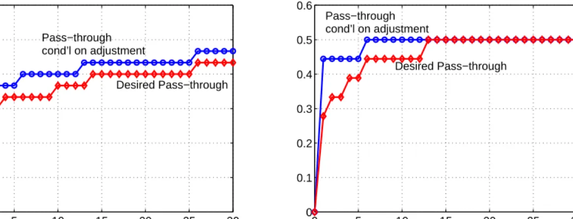
The left panel of Figure 4 plots the desired pass-through profiles {Ψ˜jt} for three firms: Firms A and B have steeper desired pass-through profiles than Firm C, which however has a higher initial desired through. As a result, Firm C has relatively high desired pass-through on impact but a lower desired long-run pass-pass-through than the two other firms. Finally, Firm B has desired pass-through strictly greater than Firm A at all horizons.
19Only 125 goods in the sample change currency during their life in the index. This empirical finding can also be consistent with small costs of changing the currency of pricing even in an environment where Assumption 1 fails.
20This observation is consistent with the finding in Gopinath and Rigobon (2007) that non-dollar firms have a slightly higher duration of prices than dollar firms.
0 2 4 6 8 10 12 0 0.2 0.4 0.6 0.8 1 t, months Firm A Firm B Frim C 2 4 6 8 10 12 0.2 0.3 0.4 0.5 0.6 0.7 0.8 Duration, months Firm A Firm B Firm C
Figure 4: Desired Pass-through profiles, ˜Ψjt (left); and corresponding Medium-run Pass-though as a function of duration, ¯Ψj0(τ) whereτ = 1/(1−θ) (right)
The right panel of Figure 4 in turn translates using (9) respective desired pass-through profiles of these three firms into our measure of medium-run pass-through, ¯Ψj0, as a function of the expected duration of firm’s price, τj = 1/(1−θj). Proposition 3 shows that ¯Ψj
0(τj) has to be compared with 1/2 to determine the currency choice. First, we observe that each firm is more likely to become LCP when its duration is low: Firm A, C and B will become LCP if their expected durations are less then 5, 4 and 3 months respectively. This illustrates Corollary 3. Next, observe that firm B for any given duration is more likely to become PCP than firm A since its desired pass-though profile is strictly higher and as a result its medium-run pass-through is also higher for any given duration. This illustrates Corollary 2.21 Lastly, note that both duration and the entire desired pass-through profile are important in determining currency choice. In the example above we cannot predict currency choice based solely on long-run pass-through or desired pass-through on impact. Specifically, firm C has a higher desired pass-through on impact than both other firms but it will switch into PCP only after firm B does so, as we increase the duration of prices. Moreover, firm A has a higher long-run desired pass-through than firm C, however it will switch into PCP only after firm C does so, as we increase the duration. This illustrates the difference in the currency choice rule in a multi-period setting as compared to a one-period ahead setting.
21We do not illustrate Corollary 1, as it is straightforward: when ˜Ψ
` ≡Ψ for all˜ `, then ¯Ψ0≡Ψ for any˜ durationτ.
3.2
Medium-run versus Long-run Pass-through
The previous section provides a sharp link between currency choice and medium-run ex-change rate pass-through without requiring to specify the determinants of pass-through. In this section, we examine two standard sources of incomplete pass-through, variable mark-ups and imported intermediate inputs so as to describe circumstances under which medium-run pass-through will differ from long-run pass-through. We also define the empirical specifica-tion to be used in the next secspecifica-tion.
First, we split the state space so that ht = (Pt, zt), where Pt is the sectoral price level (in logs) and zt are all other state variables. We assume that shocks to et affects only Pt+` for ` ≥ 0 and do not affect any leads or lags of zt.22 This assumption is introduced for expositional purposes and can be easily relaxed.
Next we write explicitly the profit function of the firm
Π¡p; (e, P, z)¢=Q(p;P, z)£exp(p)−exp¡e+c∗(e, z)¢¤, (10)
where Q(·) is demand for the firm’s exports and c∗(·) is the log of the unit cost in producer
currency. Implicitly we have assumed that the firm operates a constant returns to scale technology since the unit cost function does not depend on the price of the firm.23 Both demand and costs of the firm can be affected by shocks exogenous to the exchange rate.
The cost function can additionally be affected by the exchange rate directly if the firm uses imported intermediate inputs. We denote the elasticity of the unit cost in local currency with respect to the exchange rate by
φ≡ d[e+c∗(e, z)] de
and interpret φ as the fraction of the cost of the firm incurred in the producer’s currency.24 When φ < 1, the firm has limited incentives to adjust its local currency price since its unit cost in local currency does not move as much. This is the imported inputs channel of incomplete pass-through.
22Specifically,ztmay include idiosyncratic or aggregate productivity, overall demand conditions, and other firm-specific characteristics such as properties of production technology and menu costs of the firm.
23Decreasing returns to scale are known to generate additional channels of strategic complementarities and incomplete exchange rate pass-through (Burstein and Hellwig, 2007; Goldberg and Tille, 2005). However, empirically it is hard to disentangle this channel from the variable mark-ups channel, which we introduce below.
24Throughout the paper we will assume thatφis a constant. One example when this assumption is exactly satisfied is the case of Cobb-Douglas unit cost function with the price of first and second inputs perfectly stable in producer and local currencies respectively.
The effective elasticity of demand is given by
σ(p;P, z)≡ −d lnQ(p;P, z)
dp .
The optimal mark-up of the firm (in logs) is then µ≡ln [σ/(σ−1)].As a result, the desired price of the firm is defined implicitly by
˜
p(e, P, z) =µ(˜p;P, z) +c∗(e, z) +e. (11)
The desired pass-through of the firm is ˜ Ψ(e, P, z)≡ d˜p(e, P, z) de ¯ ¯ ¯ z = φ 1 + Γ + ΓP 1 + Γ dP de, (12)
where we denote Γ ≡ −dµ/dp and ΓP ≡ dµ/dP.25 Γ and ΓP measure the strength of strategic complementarities in the model, or the extent of what is referred to as pricing-to-market. This is the variable mark-ups channel of limited pass-through. The mechanism of variable mark-ups for incomplete exchange rate pass-through was first proposed in the seminal works of Dornbusch (1987) and Krugman (1987) and later used in multiple papers.26 Note that the sectoral price level P is an endogenous variable determined in equilibrium by the fraction of firms adjusting their price and the respective sizes of these adjustments. Conditional onz, the dynamics of the price level is determined by the shocks to the exchange rate. We will assume that dPt+`/det depends only on ` and does not depend on the initial state st. This is equivalent to Assumption 1 in the previous section. As a result,
˜ Ψ` = φ 1 + Γ + ΓP 1 + Γ dPt+` det . (13)
Finally, the long-run pass-through is ˜ Ψ∞= φ 1 + Γ + ΓP 1 + Γ dPt+∞ det , (14)
that is the response of the price of the firm to the exchange rate shock when all other firms in the sector have had enough time to adjust to this shock.27 If prices are flexible, all firms
25Many demand specifications, like that in Atkeson and Burstein (2005) and Klenow and Willis (2006), imply Γ = ΓP. For CES demand, Γ = ΓP = 0 and µ=const. In general, Γ and ΓP are necessarily related
but do not have to be equal. A reasonable assumption is that Γ≥ΓP ≥0.
26Note that when Γ = Γ
P = 0, which is in particular true under CES preferences and constant elasticity
demand, the desired pass-through of the firm is always equal to φ and does not depend on the sectoral price level and hence the prices of competitors. This means that the variable mark-up channel of incomplete pass-through is shut down. Finally, when Γ>0, the desired pass-through isφ/(1 + Γ)< φwhen the sectoral price level is held fixed (e.g., competitors do not respond to the exchange rate shock); and when ΓP >0,
desired pass-through is increasing in dP/de.
27Note that equivalently long-run pass-through can be defined as ¯Ψ
∞≡limt→∞Ψ¯t, where ¯ Ψt≡(1−δθ) P∞ `=0(δθ)`Ψ˜t+` so that indeed ¯Ψ∞= ˜Ψ∞.
adjust instantaneously, thus dPt+∞/det= dPt/detand hence ˜Ψ∞ is also a measure of flexible
price pass-through. Finally, note that if ˜Ψ` has an increasing profile, long-run pass-through is higher than medium-run pass-through. ˜Ψ` will have an increasing (decreasing) profile if most competitors of a foreign firm price in the local (producer) currency. This explains the importance of coordination motive for currency choice.28 In the case of the U.S., it is natural to assume that most competitors for a firm price in dollars.
We summarize the discussion above in
Proposition 4 If strategic complementarities are important (specifically, whenΓP6= 0), medium-run and long-medium-run pass-through are different and flexible price pass-through is not a sufficient statistic for currency choice. If the sectoral price index responds sluggishly to exchange rate shocks, then medium-run pass-through is lower than long-run pass-through.
Finally, we mention that φ, Γ and ΓP are important primitives that determine both pass-through of the firm at different horizons, as well as its currency choice. The lower is φ, the lower is the pass-through of the firm at all horizons and the firm is more likely to choose local currency pricing. Comparative statics with respect to Γ and ΓP are less unambiguous. An increase in Γ, keeping ΓP constant, will affect pass-through and currency choice in the same way as a fall in φ. However, Γ and ΓP, in most cases, are likely to change simultaneously and in the same direction. Moreover, a change in these parameters is likely to affect the equilibrium dynamic response of the sectoral price index (dPt+`/det). As a result, general predictions about the effect of Γ and ΓP on pass-through and currency choice cannot be made.29 We will investigate this link in more detail in a specific model that we simulate in Section5.
Note that we considered only a certain type of real rigidity in this section namely strategic complementarities. There are however other forms of real rigidities such as those suggested by Basu (1995) which can also rationalize long-run pass-through differing from the medium-run. In the empirical analysis, we will only provide evidence of the existence of some form of real rigidities and it is not our goal to identify the particular source of real rigidity.30
28See Krugman (1980); Goldberg and Tille (2005); Bacchetta and van Wincoop (2005). 29CES preferences and constant elasticity demand (so that Γ = Γ
P = 0) constitute one special case which
yields particularly sharp prediction. In this case,φis the only parameter that determines pass-through and currency choice: pass-through is high and PCP is optimal when φ is close 1 and pass-through is low and LCP is optimal whenφis close to 0. However, this case constitutes little theoretical or empirical interest for the purpose of explaining incomplete pass-through and currency choice.
30Delayed price adjustment to shocks can also be rationalized in a sticky information model suggested by Mankiw and Reis (2002). For a related empirical test of this model based on BLS consumer price data see Klenow and Willis (2007).
3.2.1 Empirical Specification
In this section we introduce three empirical specifications that we will take to the data in order to test the theory of currency choice.
Using (4) and (11) we write explicitly the optimal price setting rules of a firm:31 ¯ pt = (1−δθ) ∞ X `=0 (δθ)`E©µ t+`+c∗t+`+et+` ¯ ¯st, ϑ t+1=. . .=ϑt+`= 0 ª = Θ(L)[µt+c∗t +et], (15)
where Θ(L) represents the corresponding expected present value operator (conditional on non-adjusting prices) and for brevity µt+` and c∗t+` denote µ(¯pt;Pt+`, zt+`) and c∗(et+`, zt+`) respectively.
With this notation, we can write the size of the optimal price adjustment as ¯
xt≡∆τ1p¯t ≡p¯t−p¯t−τ1 = Θ(L)∆τ1[µt+`+c
∗
t+`+et+`], (16) whereτ1 is the most recent duration of the firm’s price (in the currency of price setting). In words, the size of the optimal price adjustment is equal to the revision in the expectations about the future path of optimal mark-ups, marginal costs and exchange rates. The following proposition allows us to make the transition from (16) to an empirically identifiable equation:
Proposition 5 When the exchange rate follows a random walk and up to the second order, optimal price adjustment can be expressed in local currency, irrespective of the currency of pricing, as ¯ xt = φ 1 + Γ[et−et−τ1] + ΓP 1 + ΓΘ(L)[Pt−Pt−τ1] +ε(z t). (17) Proof: See Appendix ¥
Motivated by Proposition 5, we will estimate the following three regression specifications: ¯ xt= ˆΨ0[et−et−τ1] +ε1(z t), (18) ¯ xt= ˆΨ0[et−et−τ1] + ¡ˆ Ψ1−Ψˆ0 ¢ [et−τ1 −et−τ1−τ2] +ε2(z t), (19) ¯ xL T ≡∆Lp¯T = ˆΨ∞∆LeT +ε3(zt), (20) where τ2 is the previous duration of the price of the firm and ∆L denotes a life-long change in the respective variable; specifically, ∆Lp¯T is the difference between the last and the first
31Note that, according to Proposition 1, this is the optimal local currency price for both LCP and PCP firms. A PCP firm will set ¯p∗
t = Θ(L)[µt+c∗t] in producer currency so that ¯pt= ¯p∗t+et, given that by the
observed prices of the firm and ∆LeT is the cumulative change in the exchange rate over the life of the good.
Estimated coefficient ˆΨ0 is our proxy measure for the medium-run pass-through ¯Ψ0. The theory suggests that this should be the sufficient statistic for the currency choice of firms with higher values of ˆΨ0 making the choice of producer currency pricing more likely. Further, under the null of no real rigidities, a firm should not react to exchange rate shocks that took place prior to the most recent period of non-adjustment, which implies ˆΨ1 = ˆΨ0. Conversely, when real rigidities are important, past changes in the exchange rate can effect current price adjustments of the firm through, for instance, their sluggish effect on competitors prices. Therefore, the second specification allows us to estimate the importance of real rigidities by testing the null that the coefficient on the lag of exchange rate change is equal to zero. Finally, the life-long specification produces a coefficient ˆΨ∞which we treat as a proxy for the
long-run (or flexible price) pass-through coefficient ¯Ψ∞= ˜Ψ∞. We formalize this discussion
in32
Proposition 6 (a) ΨˆLCP
0 < 1/2 < Ψˆ0P CP; (b)When real rigidities are important, Ψˆ1 6= ˆΨ0. (c)When Ψˆ0 < 1/2< Ψˆ∞, the firm should choose LCP despite a high flexible price
pass-through.
4
Micro-level ERPT and Currency of Pricing
In this section, we empirically test the implications of the theory section, as summarized in Proposition 6, for the relation between currency choice and pass-through. We also evaluate the importance of real rigidities in the data.
To test these implications, as highlighted in the previous sections, we need a measure of pass-through that is estimated from periods of price adjustment. This is an important departure from empirical studies that use aggregate price indices, as was done in Section 2. Given the low frequency of price adjustment observed in the data, aggregate price indices are dominated by unchanging prices. Increasing the horizon of estimation to several months so as to arrive at the flexible price pass-through does not solve this issue because around 30% of the goods in the BLS sample do not change their price during their life, i.e. before they get replaced. Consequently, when estimating the pass-through using the BLS index such prices have an impact on measured pass-through even at long horizons.
32We emphasize again that the particular threshold of 1/2 is specific to the quadratic approaximation. We however show in the numerical section that for certain parameter specifications 1/2 is a fairly accurate measure of the threshold.
Another advantage of examining good level price adjustments is that we can distinguish between the response of prices conditional on the first instance of price adjustment and further rounds of price adjustment, in order to test for the importance of real rigidities.
The relevant estimate of pass-through for currency choice is related to the unconditional covariance-over-variance between prices and the exchange rate. Consequently, the appro-priate regression will have no other controls besides the nominal exchange rate. To more transparently compare our regression estimates to other estimates in the literature, we will include, as is standard in the literature, a control for the foreign country inflation, domestic inflation and GDP growth. This is innocuous because the coefficient on the nominal ex-change rate for the countries in our sample ex-changes very little if we do or do not include these controls. This reflects the fact that the nominal exchange rate has very low covariance with these other variables. In all the regressions we include a fixed effect for each country and primary stratum lower pair (mostly 4 digit harmonized code) and cluster the standard errors to allow for correlation in the residuals within these pairs.
We first estimate the following equation, which is the counterpart to equation (18): ¯ xt = ˆΨLCP0 ∆τ1et+ ¡ˆ ΨP CP 0 −ΨˆLCP0 )·D·∆τ1et+Z 0 tγ1+²1,t, (21) where, as before, ¯xt is the change in the dollar price,conditional on price adjustment in the currency of pricing;33 ∆
τ1et ≡ et−et−τ1 and τ1 is the duration of the previous price in the
currency of pricing. Recall that under the random walk assumption, ∆τ1et is the proper
measure of the revision in expectations about the path of the exchange rate accumulated over the period of price non-adjustment. D is a dummy that takes the value of 1 when the good is priced in the foreign currency. Zt includes controls for the foreign consumer price level, the US consumer price level and US GDP.34
The results from estimation of specification (21) are reported in Table 2. The first row, reports the results from pooling all observations. The pass-through, conditional on a price change, to the cumulative exchange rate change, is 0.24 for dollar priced goods and 0.90 for non-dollar priced goods. Recall that these are our proxy estimates of the medium-run pass-through which, according to the theory, should be a sufficient statistic for the currency choice. The difference in these pass-through estimates is large and strongly significant, which
33In the BLS database, the original reported price (in the currency of pricing) and the dollar converted price are both reported. We use the latter, conditional on the original reported price having changed. Since the first price adjustment is censored from the data, we also perform the analysis excluding the first price change and find that the results are not sensitive to this assumption.
34The data series for these variables was obtained from the IMF’s International Financial Statistics database. For consistency, we include the cumulative change in this variables over the period of price non-adjustment. We also allow for these variables to effect pass-through differentially across dollar and non-dollar priced goods.
supports the prediction of the currency choice model. We estimate this specification for each country and obtain similarly that there is a sizeable difference in the point estimate of dollar and non-dollar priced goods. This difference is statistically significant at conventional levels of significance for 9 out of the 11 countries. The exceptions are Spain and Canada.
In Table 3 we perform the same analysis except we restrict the sample of goods to only differentiated goods, using the Rauch (1999) classification.35 We were able to classify around 65% of the goods using this classification. Here again we find strong evidence of a selection effect. The average medium-run pass-through for dollar priced firms is 0.24 and it is 0.96 for non-dollar priced firms. This difference is also observed at the country level, with the difference in the pass-through estimates being significant for all countries, except Spain and Canada.
Next, we allow for lags in the exchange rate changes to affect current price adjustment to test for the presence of real rigidities. We estimate
¯ xt = ˆΨLCP0 ∆τ1et+ ¡ˆ ΨP CP 0 −ΨˆLCP0 ¢ ·D·∆τ1et (22) + ∆ ˆΨLCP1 ∆τ2et−τ1 + ¡ ∆ ˆΨP CP1 −∆ ˆΨP CP0 ¢·D·∆τ2et−τ1 +Z 0 tγ2+. . .+²2,t, where ∆ ˆΨc
1 ≡Ψˆc1−Ψˆ0c for c∈ {LCP, P CP} and τ2 is the duration of the previous price of the firm so that ∆τ2et−τ1 ≡et−τ1 −et−τ1−τ2 is the cumulative exchange rate change over the
previous (the one before the most recent one) period of non-adjustment. In this specification we also allowZt to include lagged foreign and domestic inflation.36
Specification (22) is the counterpart to equation (19) and the results are reported in Table 4. This specification requires the goods to have at least two price adjustments during their life. Since there are several goods that have only one price change during their life, we lose about 30% of the goods when we move to this specification from (21) which required the good to have only one price adjustment during its life. Nevertheless, we obtain very similar estimates for specification (21) to those reported in Tables 2 and 3 when we estimate that specification using only the goods that enter the sample for specification (22), i.e. those that have at least two price adjustments during their life.37
From Table 4 we observe that medium-run pass-through is significantly different between dollar and non-dollar goods, as was the case in Tables 2 and 3. Moreover, quantitatively
35Rauch (1999) classified goods on the basis of whether they were traded on an exchange (organized), had prices listed in trade publications (reference) or were brand name products (differentiated). Each good in our database is mapped to a 10 digit harmonized code. We use the concordance between the 10 digit harmonized code and the SITC2 (Rev 2) codes to classify the goods into the three categories.
36We have estimated the specification with lagged own price changes and find that the implied pass-through estimates are very similar.
37This is consistent with our assumption that the exchange rate follows a random walk so that the current change in the exchange rate is uncorrelated with the previous exchange rate movements.
the estimates are very similar across these tables. In the first row of Table 4, for all goods, the difference between medium-run pass-through of non-dollar and dollar firms is 0.62 and is highly significant. This is again the case when we look at the sub-samples of Euro and Non-Euro countries. The pass-through for non-dollar goods for the Euro (Non-Euro) area is 64 (59) percentage points higher.38 This large and significant difference is also evident when we restrict the sample to differentiated goods: it is 67 percentage points in this case.
The second finding of Table 4 is that exchange rate shocks that took place prior to the current period of adjustment have a significant effect on current price adjustments. This supports the existence of strong real rigidities in pricing behavior across firms. The first row of Table 4 points out that the elasticity of current price changes to lagged exchange rate shocks for dollar priced goods is 0.21, which is only slightly smaller than the response to the contemporaneous exchange rate movement (equal to 0.25). This significant effect for dollar priced goods is documented also for the sub-sample of Euro and Non-Euro countries and for differentiated goods.39 For non-dollar priced goods the second rounds of adjustment are in general small and insignificantly different from zero. This finding is also consistent with the endogenous currency choice theory that goods with low strategic complementarities should price in producer currency.
It is important to stress that this result on real rigidities is of independent interest as it provides evidence for a mechanism that can generate significant inertia in the response of prices to shocks, much longer than the median duration of price rigidity. This is viewed as essential for generating quantitatively significant non-neutralities to monetary shocks. Evidence of this mechanism has been tested in recent papers by Klenow and Willis (2006) and Burstein and Hellwig (2007) using consumer price data. One of the useful features of international data for this purpose is that we have an observable cost shock, namely the exchange rate, that is arguably orthogonal to idiosyncratic cost-shocks of firms.
A third finding from Table 4 is that pass-through after multiple rounds of adjustment need not be as dramatically different between local and producer currency pricing firms. This refers back to the point made in Section 3 that what matters for currency choice is the medium-run pass-through and not the long-run pass-through. As is evident in Table 4, for all cases the difference between the dollar and non-dollar goods after two rounds of adjustment is substantially lower than after one round of adjustment. For all goods, the
38There are not enough observations to perform a country-by-country analysis. For Germany and Japan for which there are sufficient observations for both dollar and non-dollar goods we obtain similar results to those reported in Tables 2 and 3.
39For the Euro (non-Euro) countries the elasticity of current price change to lagged exchange rate move-ments is 0.14 (0.24) as compared to 0.23 (0.24) for contemporaneous exchange rate change. Similarly, for the sample of differentiated goods the ‘lagged’ elasticity is 0.21 versus the ‘contemporaneous’ of 0.22.