© 2006 International Monetary Fund
Exchange Rate Pass-Through in the Euro Area
HAMID FARUQEE*Exchange rate pass-through in a set of euro area prices along the pricing chain is examined in this paper. First, a vector autoregression (VAR) approach is used to analyze the joint time-series behavior of the euro exchange rate and a system of area-wide prices in response to an exchange rate shock. Second, the impulse-response functions from the VAR estimates are used to identify—in a “new open-economy macroeconomics model”—the key behavioral parameters that best replicate the pattern of exchange rate pass-through in the euro area. A key finding is that traded goods—both extra-area exports and imports—behave as though they are predominately priced in euros. The area-wide findings are compared with those for other major industrial economies.[JEL F41, F31, E31]
A
gainst the backdrop of strong global growth, a low-flying recovery in the euro area has struggled to gain altitude, weighed down in part by a sub-stantially stronger euro that had appreciated by roughly 45 percent against the U.S. dollar and 25 percent on a trade-weighted basis over the past three years (since its 2002:Q1 trough) before retreating some in mid-2005. With a struggling recovery, European concerns about the economic impact of past euro appreciation have fig-ured prominently. Specifically, in the context of low area-wide inflation and soft domestic demand, the possible effects of recent exchange rate movements on inflation and trade have taken on renewed interest and significance. In assessing the likely consequences, a key determining factor is the nature of exchange rate pass-through in the euro area.*Hamid Faruqee is a Senior Economist in the European Department of the International Monetary Fund. Special thanks are due to Susanna Mursula for her outstanding research assistance and to Bankim Chada, Ehsan Choudhri, Dalia Hakura, Albert Jaeger, and Alessandro Rebucci for helpful discussions and comments.
More difficult to assess, however, are the behavioral features that underlie the nature and extent of pass-through and the responsiveness of trade flows to the exchange rate. The relevance of exchange rate pass-through for inflation is straightforward. But these issues are also important in determining the strength of expenditure-switching effects from relative price signals.1Incomplete pass-through, for example, could delay or diminish the response in external variables and pro-duce a certain degree of “exchange rate disconnect.”2Thus, ascertaining the degree of and underlying behavior behind pass-through in the euro area is a key input for assessing its likely economic impact on growth and inflation.
Several economic explanations have been put forth to account for incomplete exchange rate pass-through—a feature that has strong empirical support for a large number of economies, including the euro area.3With nominal rigidity and local currency pricing (LCP), destination prices can change very little in the face of exchange rate variation.4 With pricing-to-market behavior, segmented markets allow firms to stabilize their destination prices (via changing markups) to preserve foreign market share. In the presence of local distribution costs, firms may also face offsetting factors when the exchange rate changes, leading to international price discrimination and incomplete pass-through.5These factors can help account for differential responses between first-stage pass-through (e.g., in import prices) and second-stage pass-through (e.g., in consumer prices). Moreover, these consid-erations have been shown to have important implications for optimal monetary and exchange rate policies.6
This paper examines exchange rate pass-through and its behavioral determi-nants in the euro area. The methodology proceeds in two parts. First, the empirical analysis follows a vector autoregression (VAR) approach, in which the time-series behavior of the euro exchange rate and a system of euro area prices are examined. Specifically, the empirical analysis investigates exchange rate pass-through in a setof prices along the pricing chain. Second, the impulse-response functions (IRFs) from the VAR estimation are used to calibrate in a new open economy macro-economics model the key behavioral parameters that can help reproduce the pat-tern of pass-through and expat-ternal adjustment in the euro area.
The use of a VAR approach to examine exchange rate pass-through has several advantages compared with single-equation methods. Previous studies typically have focused on pass-through into a single price (e.g., import or consumer prices) with-out further distinguishing between the types of underlying exchange rate shocks (e.g., permanent or transitory) that may be arriving. By investigating exchange rate pass-through into a set of prices along the pricing chain, the VAR analysis charac-terizes not only absolute but relative pass-through in upstream and downstream
1See Obstfeld (2002) and Engel (2002) for recent reviews of these issues. 2See Krugman (1989) and Devereux and Engel (2002).
3See Goldberg and Knetter (1997) for a survey. See Kieler (2001), Hüfner and Schroder (2002),
Anderton (2003), and Hahn (2003) for euro area estimates.
4See Betts and Devereux (1996, 2000) and Devereux and Engel (2002). 5See Corsetti and Dedola (2002) and Choudhri, Faruqee, and Hakura (2002). 6See, for example, Corsetti and Pesenti (2002) and Devereux and Engel (2003).
prices. Second, the VAR methodology potentially allows one to identify specific structural shocks affecting the system. In this case, a structural exchange rate shock is identified through a Cholesky decomposition of innovations, in which exchange rate fluctuations at higher frequencies are assumed to be largely driven by asset market—rather than goods market—disturbances.
Using this identification scheme, one can map the empirical results into a well-defined shock in an economic model of incomplete pass-through. Specifically, the estimated IRFs from an exchange rate shock in the VAR are matched to the rela-tive response patterns generated by the corresponding asset market disturbance in the analytical pass-through model. By minimizing the distance between these sets of IRFs, one can identify key structural parameters that underlie the overall pat-tern of pass-through. The key parameters include (1) the pricing behavior of firms (i.e., the extent of local currency pricing), (2) the degree of nominal rigidity, and (3) the extent of local distribution and trading costs generating international price discrimination. A comparison of these behavioral parameters across the major industrial countries can then be made.
I. Empirical Estimates
The empirical analysis focuses on euro area prices and the exchange rate at a monthly frequency. The time span covers the period from 1990 through 2002. All series are expressed in logarithms. For the euro exchange rate s,the nominal effec-tive series is defined for the European Central Bank’s “narrow” group of partner economies.7For factor prices (i.e., wage earnings w), the series derive from quar-terly data on nominal compensation per employee, extrapolated to a monthly fre-quency.8For trade prices, import prices pmand export prices px are based on unit values in extra-area manufacturing trade.9Producer prices pyare based on the pro-ducer price index for manufacturing, excluding construction and energy. Consumer prices pcare based on the core consumer price index (CPI)—that is, excluding energy and unprocessed foods—from the harmonized index of consumer prices (HICP), although the implications with headline inflation are also discussed.10The exclusion of energy prices is motivated primarily by the standard finding that their pass-through behavior differs from that of other goods; by eliminating them, we facilitate a more seamless transition to the pass-through model later that emphasizes differentiated goods with imperfect substitutability.11
7Partners are Australia, Canada, Denmark, Hong Kong SAR, Japan, Korea, Norway, Singapore, Sweden,
Switzerland, the United Kingdom, and the United States.
8Price and wage data are from Eurostat and are not seasonally adjusted. The areawide measures reflect
aggregates of the 11 participating countries through December 2000. Thereafter, the chained series include Greece as the 12th member country.
9Manufactured goods include Sections 5–8 of the Standard International Trade Classification. The use
of unit values (i.e., aggregrate, implicit deflators) is not ideal, but data limitations on direct trade prices necessitate their use.
10For Canada, Japan, the United Kingdom, and the United States, all corresponding monthly series
were drawn from the IMF’s International Financial Statistics,except wages, which were obtained from the Organization for Economic Cooperation and Development’s Analytical Database.
The use of extra-area trade data helps avoid potential pitfalls from inferring pass-through for the euro area from estimates for individual member countries. To the extent that intra-area trade systematically differs from extra-area trade with respect to pass-through behavior, aggregating country estimates to generate an areawide measure could suffer from a “fallacy of composition.” Hüfner and Schroder (2002), for example, construct pass-through estimates for euro area con-sumer prices by summing over individual country estimates, based on each coun-try’s weight in the areawide HICP. The analysis is then forced to make some “correction” of the estimates due to the presence of intra-area trade.
Before turning to the VAR estimation of euro area pass-through, some pre-liminary tests of the data were conducted. Unit root and stationarity tests indicate that these nominal variables are nonstationary in levels but stationary in first dif-ferences, suggesting that they are integrated-of-order-one or I(1) series.12 Further-more, residual-based co-integration tests do not find evidence of co-integration among the variables (see Appendix). Given potential nonstationarity and lack of co-integration in the data in levels, estimating the VAR in first differences is appropriate.
VAR Methodology
The VAR approach examines the joint historical time-series behavior of the euro exchange rate and a system of euro area prices. Specifically, the reduced-form VAR(p) can be written as follows:
where Y=[∆s ∆w∆pm∆px∆py∆pc]′; c is a vector of deterministic terms (i.e., monthly time dummies); Ais a matrix polynomial of degree pin the lag operator L; and µ is the (6 × 1) vector of reduced-form residuals with variance-covariance matrix Ω. The exchange rate is placed first in the order of variables, reflecting the presumption that exchange rate innovations at monthly frequency are primarily driven by exogenous asset market disturbances.13For prices, the ordering after the exchange rate is motivated by the pricing chain, from factor input prices to trade prices to wholesale producer prices and retail consumer prices. The ordering among price variables after the exchange rate does not matter for the subsequent analysis of the exchange rate shock.
Y c A L Y E t t t t t = + ( ) + ′
[
]
= −1 1 µ µ µ ; , ( ) Ω12The differenced series for euro area consumer and import prices were borderline nonstationary (see
Appendix). But, as is well known, unit root and stationarity tests have low power, making it difficult to dis-tinguish between stationary and unit root processes in finite samples.
13The identification scheme largely follows Choudhri, Faruqee, and Hakura (2005). That analysis also
includes the interest rate in the VAR in order to further distinguish between the effects of interest rate and exchange rate shocks on prices. McCarthy (2000) and Hahn (2003) also use a Cholesky decomposition to examine pass-through based on a somewhat different model.
To recover the underlying exchange rate shock, the Cholesky decomposition of the matrix Ωis used to produce orthogonalized innovations ε. These disturbance terms are expressed in terms of the reduced-form VAR innovations as follows:
where Cis the unique lower triangular Cholesky matrix with 1salong its principal diagonal. Because the exchange rate appears first in the VAR, the recursive struc-ture in equation (2) imposes the assumption that orthogonalized innovations to the exchange rate depend only on the residuals from the exchange rate equation and not from the other equations. This identification allows for a simple correspon-dence between the VAR estimates and a well-defined shock in the model described later. For prices, the corresponding disturbance term will represent a mix of shocks, including the structural exchange rate shock.14
An alternative identification scheme would place the exchange rate last (or near last) in the VAR. This ordering is motivated by the view that prices (and quan-tities) are predetermined in the very short run and, thus, cannot respond to an exchange rate shock; whereas the exchange rate can respond to various shocks.15 Although this restriction may be valid for many prices, it may not be appropriate for others. More to the point, this ordering imposes a specific pass-through pattern in the estimates and, ultimately, certain behavioral features in the model that the current analysis seeks to investigate. Nevertheless, sensitivity analysis is reported later for reorderings of the VAR.
The implications of the identifying restriction can be further understood from the structural representation of the VAR:
where F(L) is a matrix polynomial of degree p+1, kis a transformation of deter-ministic terms (i.e., Ck=c), and εis the vector of structural shocks. One can show that the identification scheme based on the Cholesky decomposition introduces the following restriction: In the first equation (i.e., for the exchange rate ∆s), the coef-ficients on contemporaneous price changes ∆w,∆pm,∆px,∆py,and ∆pcare equal to zero. Granger causality and block exogeneity tests find that (lagged) euro area prices have no predictive value for the euro exchange rate.16The VAR identifica-tion scheme takes this result one step further, assuming that concurrent price inno-vations also do not help explain exchange rate innoinno-vations.
F L Y( ) t= + εk t, ( )3
Cεt=µt, ( )2
14For the first variable (i.e., the exchange rate), the orthogonalized disturbance term is given by ε 1t=µ1t.
For the jth variable (j> 1) in the VAR, the corresponding shock term is given by εjt=µjt−cj,1εjt. . .
−cj,j−1εjt, where cj,icorrespond to the entries of the Cholesky matrix (see Hamilton, 1994).
15See, for example, Peersman and Smets (2001).
16The exchange rate, however, helps predict (at least) trade prices (see Appendix). Restricted VAR
estimates (not reported) excluding lagged prices from the exchange rate equation yield very similar results to those reported here.
The economic justification for this identifying assumption can be understood as follows. Exchange rates—especially at higher frequencies—are essentially driven by asset market rather than goods market disturbances. In the presence of noise traders, these short-run fluctuations may have little to do with economic fun-damentals, including the price variables considered here.17 The econometric assumption, though, is not necessarily incompatible with a more “fundamentalist” view. Under the asset market view of exchange rate determination, the predictable component is usually deemed small, and short-run changes in the exchange rate are likely to be dominated by “news.”18In the universal presence of reporting lags, however, data releases on price indices, when they are made available, typically offer very little new information to move exchange rate markets. Furthermore, the empirical justification for this identification scheme is well known, given the over-whelming failure of exchange rate models to outperform a simple random walk over short horizons.19
Based on the reduced-form estimates of the VAR and the Cholesky decompo-sition to identify structural shocks, accumulated IRFs to a unit exchange rate shock are shown in Figure 1.20The horizontal axis measures the time horizon in terms of months after the shock; the vertical axis measures the deviation in (log) prices from their baseline levels.
Figure 1 shows that the impact effects of an exchange rate shock on prices are small in the euro area. Prices tend to be predetermined or very sticky (in local cur-rency) initially in response to a depreciation in the euro effective exchange rate. Over time, the degree of exchange rate pass-through generally rises, although min-imally so in factor and retail prices. Wholesale producer prices tend to rise more than retail consumer prices, but the greatest response is in trade prices. Twelve to 18 months after the shock, export prices respond by almost half the response in import prices, which moves in proportion to the exchange rate, suggesting full pass-through. Consequently, the (manufacturing) terms of trade for the euro area tend to worsen or decline in response to an exchange rate depreciation.21Choudhri, Faruqee, and Hakura (2005) report similar relative pass-through findings in a quar-terly VAR for Group of Seven (G-7) countries that further include interest rates to account for monetary policy shocks.22
17See, for example, Jeanne and Rose (2002) and Devereux and Engel (2002). 18See Mussa (1984).
19See the seminal paper by Meese and Rogoff (1983). More recently, see, for example, Flood and Rose
(1995) and Cheung, Chinn, and Pascual (2002). For a review, see Sarno and Taylor (2002).
20Given the large number of parameters in the VAR, a parsimonious lag structure is sought to conserve
degrees of freedom. The lag length pis chosen by starting with given maximum lag length and sequen-tially testing the incremental significance of dropping an additional lag based on the likelihood ratio test. Derived from bootstrapping methods, confidence intervals for the IRFs are shown in Figure 3.
21Obstfeld and Rogoff (2000) provide evidence that the terms of trade decline with a currency
depreciation—an observation that appears at odds with the implications of strict LCP models. See Lane (2001) for a review.
22The exchange rate path is typically found to be less persistent (i.e., more mean-reverting) in the
quar-terly VAR when interest rates are included (and first in the ordering), but the (absolute and relative) pass-through effects are more similar to those reported here.
Normalizing the price responses in Figure 1 by the path of the exchange rate response, Table 1 shows dynamic pass-through elasticities for euro area prices. After 18 months, pass-through rates in export and import prices are about one-half and one, respectively. Wage pass-through is relatively very small at 5 percent. Pass-through in wholesale prices is nearly 20 percent, significantly exceeding the pass-through in retail prices.23Using headline rather than core inflation (or includ-ing longer lags) would raise the degree of pass-through in consumer prices to near 10 percent at 18 months, but the pattern of relative pass-through remains intact.
Full pass-through in euro area import prices over time may be a somewhat sur-prising result.24Alternative specifications (e.g., with coefficient restrictions or VAR reorderings) tend to yield smaller but still high pass-through elasticities between 0.7 and 1. In a recent paper that also examines extra-area manufacturing trade prices, Anderton (2003) also finds generally high (albeit not full) pass-through between 0.5 and 0.7, based on a single-equation approach.25Given the identifica-tion of near-permanent exchange rate shocks here, it is not surprising that import
Figure 1. Exchange Rate Shock on Euro Area Prices
23Gagnon and Ihrig (2001) find low degrees of pass-through (around 5 percent) in consumer prices for
20 industrial countries, and argue that pass-through has been declining.
24These estimates should be taken as indicative, given the standard errors of the impulse-response
functions. Based on bootstrapped standard errors, the 90 percent confidence interval for import prices is the widest, suggesting pass-through at 18 months in the range 0.6 to 1.4. The median value of this band suggests a slightly lower degree of import price pass-through (i.e., 0.95 at 18 months); otherwise, the median and estimated IRFs closely coincide.
25The time pattern is similar, though, with most of the price adjustment transpiring by five quarters.
Based on a quarterly VAR, Hahn (2003) reports similar findings on the degree and time pattern of pass-through in the euro area non-oil import deflator.
–1.0 –0.8 –0.5 –0.3 0.0 0.3 0.5 0.8 1.0 0 6 12 18
Months after shock
Consumer prices Import prices Wages Export prices Terms of trade Producer prices
price pass-through in this VAR analysis lies somewhat above those single-equation estimates.
Cross-Country Evidence
Before relating the empirical findings to the theoretical model, it is useful to compare the pass-through results for the euro area to the other major industrial economies. Repeating the VAR exercise for the United States, Japan, the United Kingdom, and Canada produces the pass-through coefficients for trade prices shown in Table 2.
Table 2. Pass-Through Elasticities in Trade Prices: International Comparisons
t=1 t=6 t=12 t=18 Import Prices Euro area 0.03 0.42 0.81 1.17 United States 0.06 0.15 0.18 0.30 Japan 0.61 0.56 0.57 0.57 United Kingdom 0.28 0.58 0.57 0.60 Canada 0.68 0.54 0.62 0.68 Export Prices Euro area 0.02 0.18 0.31 0.45 United States 0.00 0.00 0.06 0.12 Japan 0.62 0.50 0.48 0.47 United Kingdom 0.16 0.47 0.46 0.50 Canada 0.35 0.19 0.35 0.44
Source: IMF staff estimates.
Notes: Based on impulse-response functions from six-variable VAR estimated from 1990 through 2002. For euro area, import and export prices are based on unit values in manufacturing trade. For others, import and export prices are based on unit values in total trade.
Table 1. Euro Area Pass-Through Elasticities
(Percent change in prices divided by percent change in exchange rate)
t=1 t=6 t=12 t=18 CPI 0.00 0.01 0.02 0.02 PPI 0.00 0.04 0.11 0.17 Wage −0.02 0.04 0.07 0.05 Px 0.02 0.18 0.31 0.45 Pm 0.03 0.42 0.81 1.17
Source: IMF staff estimates.
Notes: CPI refers to consumer price index; PPI refers to producer price index; Wage refers to nominal compensation per employee; Pxand Pmrefer to export and import prices. Based on impulse-response functions from six-variable vector autoregression (VAR) estimated on monthly data from 1990 through 2002.
As evident from the table, pass-through is incomplete, particularly in the short run. For the United States, pass-through in trade prices at the time of the shock is near zero, quite similar to the response of euro area. But while pass-through rises significantly over time in the euro area, the increase is much smaller for the United States. For the other countries, pass-through to import and export prices is higher on impact than for the United States and the euro area. For Canada and Japan, import price pass-through estimates are about 60–70 percent initially and remain around those levels over time; for the United Kingdom, import price pass-through eventu-ally reaches 60 percent, but is initieventu-ally half that. Pass-through in export prices is eventually around 50 percent for these three countries, similar to the euro area. Sensitivity Analysis
As is well known, impulse responses from a VAR can be sensitive to the ordering of variables. In the six-variable VAR system, there are 6!=720 possible orderings under the Cholesky decomposition used to identify structural shocks. In general, when the reduced-form residuals from the VAR do not display high cross correla-tions, the order of factorization makes little difference.26Otherwise, the results can be sensitive to the choice of ordering. Since the focus here is solely on the effects of an exchange rate shock, suborderings among the price variables—given the exchange rate’s order in the VAR—do not matter. Thus, the relevant reorderings to consider surround the placement of the exchange rate in the VAR and the combi-nations of price variables selected to appear either before or after the exchange rate, given its order in the VAR.27
Changes taken from this subset of possibilities, however, can be shown to have very little impact on the results for the euro area (and the United States); the results are robust to reorderings of the VAR. Take the extreme cases. Compared with the case in which the exchange rate appears first in the VAR, placing the exchange rate last in the VAR produces very similar pass-through elasticities for the euro area (see Appendix).28 Similarly, placing different combinations of prices before or after the exchange rate does not materially affect the results. For the other coun-tries, the results largely obtain so long as the trade prices appear after the exchange rate in the VAR. Otherwise, import and export prices would be predetermined (i.e., have zero response on impact) by construction,which, as shown in Table 2, does not reflect their behavior under less restrictive assumptions. Given the objec-tive of investigating without prejudice the pass-through behavior in these key prices, making fewer (possibly erroneous) data restrictions a priori is clearly desirable.
26From the variance-covariance matrix, the correlations between residuals are less than 0.2, with the
notable exceptions of the exchange rate and trade prices and between trade prices themselves.
27This reduces the number of relevant reorderings considerably. The possible cases can be enumerated
as follows: where nCrdenotes “nchoose r.”
28The pass-through results are very similar despite the fact that the impulse-response path for the
exchange rate itself differs across the two orderings, displaying less persistence in the latter case where the exchange rate shock depends recursively on the reduced-form residuals from all the price equations. The interpretation of the exchange rate shock becomes more difficult in this case, since it incorporates a mix of innovation terms. 5 32 0 5 Cx= = ∑x ,
II. Model of Incomplete Pass-Through
This section describes the analytical framework used to interpret the VAR evidence in terms of underlying economic behavior. The stylized model generates incom-plete pass-through by drawing on many of the common themes found in the new open economy macroeconomics (NOEM) paradigm, following the seminal work of Obstfeld and Rogoff (1995).29A detailed derivation of the microfounded model can be found in Choudhri, Faruqee, and Hakura (2005). A sketch of the model follows. Imperfect competition characterizes the production and allocation of two dif-ferentiated goods—a traded intermediate good and a nontraded final (consump-tion) good. One differentiated primary factor (labor) and intermediate inputs enter the production of traded goods. A domestic retail sector relying on labor services is needed to transform intermediate goods into final consumption goods in each country. This structure gives rise to a pricing chain with five price indices: retail consumer prices, wholesale producer prices, import and export prices, and factor prices (i.e., wages).
Beginning with the demand side and consumer preferences from the home country’s perspective, expected lifetime utility of a household, indexed by l∈[0, 1], is assumed to be
where Cτ(l) and Lτ(l) are the household’s consumption basket and labor supply. The consumption basket, reflecting household preferences, is a constant-elasticity-of-substitution (CES) aggregate over individual varieties, indexed by c∈[0, 1], of the final good and is given by
Each consumption good variety, meanwhile, is produced according to the follow-ing technology:
where Qt(c) is an index of both home and foreign varieties of the intermediate good, and NCt(c) is a bundle of differentiated labor services. This technology com-bines traded goods with nontraded labor services to produce consumption services. The technology for producing a home variety, indexed by y,of the intermediate good is given by:
Y yt( )=Z yt( )αNY t( )y −α 1 7 , ( ) C ct( )=Q ct( )γNCt( )c −γ 1 6 , ( ) Ct= C ct( )− dc − ( )
∫
1 1 0 1 1 5 ε ε ε . ( ) Et C l L l t tβ ρ µ τ τ τ ρ τ µ − = ∞ − +∑
− ( ) − + ( ) 1 1 1 1 1 1 , (( )4where Zt(y) and NYt(y) are composites of differentiated intermediate and labor inputs. From these two equations, note that intermediate goods (indexed by Q) are used directly in the production of the final consumer good, while others (indexed by Z) are used in the production of other intermediate goods.
Specifically, each home intermediate variety is allocated across the following four sectors:
where YQHt(y) and YZHt(y) denote the amounts of the home variety yused to meet domestic final and intermediate demands, and Y*QMt(y) and Y*ZMt(y) denote the exports of the home variety yused to satisfy foreign final and intermediate demands. Using YQMt(y*) and YZMt(y*) to denote the corresponding amounts of an imported foreign variety, indexed by y* ∈[0, 1], the intermediate CES input bun-dles in the home country are defined as
Here, the elasticity of substitution σbetween domestic and foreign baskets of the intermediate good is allowed to be different than the elasticity εbetween varieties within each bundle. Similar equations would apply to the foreign country.
Imported varieties (in both countries) are also assumed to go through distri-bution channels before their use, and the distridistri-bution process requires local labor services. Following Corsetti and Dedola (2002), one unit of an imported variety y* in the home country requires δunits of the labor service bundle, NMt(y*), so that30 NMt( )y* =δ
[
YQMt( )y* +YZMt( )y* .]
( )13 QHt =∫
YQHt( )y dy ZHt= YZHt(y − (−) 0 1 1 1ε ε ε1 , ∫
01 ))1 1− εdyε ε(−1). (12) QMt =∫
YQMt( )y dy ZMt= YZMt − (−) * * , 0 1 1 1ε ε ε1 yy* dy* , ( ) ( ) − − ( )∫
1 1 0 1 1 11 ε ε ε Zt=[
v ZMt− + −( v) ZHt−]
− ( ) 1 1 1 1 1 1 1 1 10 σ σ σ σ σ σ , ( ) Qt=[
v QMt− + −( v) QHt−]
− ( ) 1 1 1 1 1 1 1 1 9 σ σ σ σ σ σ , ( ) Y yt( )=YQHt( )y +YZHt( )y +YQMt* ( )y +YZMt* ( )y , ( )830The Leontief-type distribution process is needed only for moving intermediate goods across
bor-ders. For simplicity, the distribution cost for imports is the same whether they are used in the production of the intermediate or the final good. Note, however, that the consumption “technology” in equation (6) specifies a Cobb-Douglas process for transforming both home and foreign intermediates into a final con-sumer good.
Firms that face these local trading or distribution costs δhave an incentive for pricing to market (PTM) or price discrimination across local and export markets.31 With this dependence on local currency wages, changes in the exchange rate lead to incomplete pass-through in trade prices and the PTM behavior described by Krugman (1987) through a cost or supply mechanism.32The introduction of pric-ing to market along these lines helps limit the effects of import price pass-through in retail prices and helps generate greater overall persistence in the degree of incomplete pass-through over time.33
Given this structure, household labor supply employed in the production of intermediate and final goods and distribution services,
and aggregate labor service bundles in the three activities are combined as follows:34
Marginal costs for final and intermediate goods derive from the employment of labor services and the costs of intermediated goods. From the production technolo-gies in equations (6) and (7), these are
where PQtand PZtare the familiar price indices associated with the CES bundles for intermediate inputs Qtand Zt in equations (9) and (10), and Wtis the aggre-gate wage.
Given the CES demands for each variety derived (ultimately) from household preferences, monopolistically competitive firms set price as a markup over marginal costs to maximize profits. But prices and wages are not fully flexible. Instead, they
MCCt=P WQtγ t−γ
(
γγ( −γ)−γ)
MCYt =P WZtα t−α αα 1 1 1 1 , ( (11−α)1−α), (16) NYt = LYt( )l − dl NCt= LCt( )l d − −∫
1 1 0 1 ε ε ε 1, 1 1ε ll NMt LMt l dl 0 1 1 1 1 0 1 1∫
∫
= ( ) − ( ) − − ε ε ε ε ε , (( ) . ( )15 L lt( )=LYt( )l +LCt( )l +LMt( )l , (14)31Investigating extra-area import prices, Anderton (2003) finds that foreign suppliers attach a
signifi-cant weight to the PTM strategy in efforts to maintain market share. Herzberg, Kapetanios, and Price (2003) find PTM to be the dominant consideration for U.K. import prices. Kieler (2001) provides com-parative estimates for several industrial countries.
32See also Kasa (1992) and Faruqee (1995) for analyses that introduce market-specific costs as a way
to generate incomplete pass-through and PTM behavior. An alternative approach focusing on varying markups and demand elasticities through translog (i.e., non-CES) preferences can be found in Bergin and Feenstra (2001).
33The home import price (in local currency terms) of a foreign variety, after and before distribution
costs, is P~Mt(y*) =PMt(y*) + δWtand thus depends partly on the domestic wage W.
34Individual labor demands facing households depend on relative wages and aggregate labor demand:
Ld
are updated only infrequently based on Calvo-type adjustment.35Specifically, the (fixed) probability that a firm will leave its price unchanged at a point in time is equal to π. Correspondingly, the average interval over which prices remain fixed is π/(1 − π).36This framework generates staggered price-setting behavior in the economy.
With nominal rigidity in an open economy, the question arises as to whether prices are sticky in terms of domestic or foreign currency. The two limiting cases are referred to as (1) local currency pricing (LCP), in which all prices are rigid in the destination or buyer’s currency; and (2) producer currency pricing (PCP), in which all prices are rigid in the origin or seller’s currency. Allowing for a hybrid case, both types of pricing behavior are nested in the model. Specifically, the param-eters φ and φ* denote the share of domestic and foreign firms following PCP behavior respectively. If φ =1, one has strict PCP; φ =0 represents strict LCP.
In the PCP case, a home producer would set its home export price PXt(y) at the point of origin; under LCP, the same firm would set the foreign import price P*Mt(y) at the destination, where P*Mt(y) =PXt(y)/St and St is the nominal exchange rate. Using superscripts Pand L to denote prices setting under each type of behavior, the values XPYt and XPXt represent (under PCP) the domestic and export contract prices under Calvo-type adjustment chosen by firms at time tto maximize the present discounted value of profits:
where DRt,τis the stochastic discount rate (consistent with preferences), πτ −tis the probability that a price set at twill remain in place at τ, and the square-bracketed expressions represent the domestic and foreign demands for the home variety, con-ditional on the price set at t.37The analogous objective functions under LCP (and for retail firms) can be similarly derived.
Solving equation (17) and its analog for retailers and for foreign firms—and under both PCP and LCP—yields the following central (log-linearized) pricing equations for aggregate producer, consumer, import, and export prices:
pC t, =πpY t,−1+ −(1 π)xC t,, (19) pY t, =πpY t,−1+ −(1 π)xY t,, (18) Et DRt X MC Z Q P X t t Yt P Y H H Y Yt ,τ τ τ π τ τ τ τ − = ∞
∑
(
−)
( + ) PP Xt P Y M M M Xt P X MC Z Q P X(
)
{
+(
−)
(
+)
−ε τ *τ *τ *ετ(
SSτ+δ*Wτ*)
−ε}, (17)35See Calvo (1983). See Kollmann (2001) for a NOEM analysis with sticky wages and prices but
with-out distribution costs.
36Choudhri, Faruqee, and Hakura (2002) also examine the cases of wage and/or price flexibility (i.e., π =0) and find that these model variants generally fall short in explaining the empirical impulse-responses.
37The firms’ stochastic discount factor is consistent with that of households, based on the Euler
con-dition in consumption: DR P C where ris the rate of interest.
P C E P C P C t t Ct t C t Ct t C t , , τ τ ρ τ τρ ρ β β = − + and 1 tt+1= +rt 1 1 ρ ,
where lowercase letters denote logarithms of variables. In the presence of Calvo-type staggered price adjustment, aggregate price indices display inertial dynamics depending on the parameter related to the probability of price (non)adjustment π. In the import and export price-setting equations, the behavior is also influenced strongly by the shares φ, φ* of LCP versus PCP firms. The underlying contracted prices (or components) entering these expressions are given by
The last equation (and its counterpart, x*D,t) reflects the role of distribution costs in the setting of trade prices, where ψCDis a weight related to the importance of unit distribution costs δrelative to marginal production costs for imports.38Along with a similar inertial equation for wages, equations (18)–(21) represent the major behavioral price-setting equations in the model, and θ ={φ, φ*, π, δ} is the vector of key structural parameters used to help map model dynamics into those gener-ated by the VAR with respect to exchange rate pass-through.
To close the model, monetary policy is determined by an interest rate rule, and uncovered interest rate parity is assumed to hold (up to an error term):
where ξrepresents an exchange rate shock, perhaps reflecting the impact of noise traders.39 st=E st t+1+rt*− +rt ξt, (27) rt=ϕ0+ϕ1rt−1+ϕ2E pt∆ Ct+ϕ3∆st, (26) xD t, =βπE xt D t,+1+ −(1 βπ ψ) CD
(
wt− −st mc* .Y t,)
(25)) xS t, =βπE xt S t,+1+ −(1 βπ)st, (24) xC t, =βπE xt C t,+1+ −(1 βπ)mcC t,, (23) xY t, =βπE xt Y t,+1+ −(1 βπ)mcY t, , (22) pX t, pY t, st pM t, pY t st * , = + −(1 φ) +π(
−1− −1+φ −1)
+(1−−π)xD t, − −( φ)xSt * , ( ) 1 21 pM t, pY t, st pM t pY t st * * , , * * = +φ +π(
−1− −1−φ −1)
+ −(1 ππ)xD t, + −(
φ)
xSt * , ( ) 1 2038Specifically, one can derive evaluated at steady-state values. Details of the
log-linearization are available from the author upon request.
39In a noise-trader model, market participants can be subject to a stochastic bias in their expectations,
Eftst+1−Etst+1= ξt, generating a UIP or exchange rate shock in equation (27).
ψ δ ε δ ε CD Y W MC S W = + * ,
Benchmarks for parameters held fixed in the model follow the calibration in Choudhri, Faruqee, and Hakura (2005), and are generally based on average esti-mated values for the major industrial countries—including euro area members Germany, France, and Italy.40Monetary policy, for example, is specified by an interest rate rule targeting expected inflation in consumer prices and allowing for interest rate smoothing, with the corresponding parameter weights based on the average estimates for the (non-U.S.) G-7 countries.
III. Matching Theory and Empirics
To match the empirical impulse-response patterns, an asset market shock ξ to uncovered interest rate parity (UIP) in the model is considered. The scale and per-sistence of ξis calibrated to reproduce the VAR’s accumulated impulse-response path for the exchange rate from a structural exchange rate shock εs.41Simulating the model’s price responses to this UIP shock generates the analytical impulse-response functions. To find the optimal structural parameter values in the model consistent with the empirical evidence, the following loss function is minimized:42
where IR(P,ξ; θ) denotes the vector of simulated impulse responses for the price vector P={w, px, pm, pc, py} from an ξshock in the model conditional on the key set of structural parameters θ = {φ, φ*, π, δ}.43 IRVAR(P, εs) denotes the corre-sponding vector of accumulated impulse responses to a structural exchange rate shock εsin the VAR. The time horizon for the impulse-response paths is 18 months. Figure 2 displays the combinations of LCP and PCP behavior in domestic and foreign firms that best replicate the price responses—particularly for trade prices— derived from the VAR estimates for each of the major industrial economies. The vertical axis measures the extent of PCP behavior φ* in foreign firms (i.e., pro-ducing home imports), and the horizontal axis measures the extent of PCP behav-ior φin domestic firms (i.e., producing home exports).
In the figure, the origin represents local currency pricing at home and abroad, while the opposing corner represents the case of universal producer currency pric-ing. The 45-degree line connecting them reflects symmetric combinations of local
min{ }θ
[
IR P( , ;ξ θ)−IRVAR(P,εs)]
′ IR P( , ;ξ θ)−IR VAAR s P,ε , ( ) ( )[
]
2840Reflecting the higher (monthly) frequency, the discount factor and interest rate are adjusted to
pro-duce consistent annualized rates with Choudhri, Faruqee, and Hakura (2005).
41The exchange rate shocks from the VAR have permanent or highly persistent effects on the log level
of the exchange rate. Consequently, the ξshocks in the model are constructed to be permanent or highly persistent as well.
42The standard errors for the accumulated impulse-response trajectories are similar, suggesting that
minimizing the unweighted least squares should yield parameters broadly similar to the weighted least squares approach used in Smets and Wouters (2002). The weighted approach would give less weight to import prices in favor of consumer prices.
43The elasticity of substitution σbetween traded goods, broadly defined, was also chosen to minimize
the distance between IRFs and found to be fairly low (σ =2), in line with Choudhri, Faruqee, and Hakura (2002); Smets and Wouters (2002); and the references cited therein. The elasticity of substitution θbetween specific varieties was also allowed to vary within a range (θ =4 to 10), consistent with plausible markups.
and producer currency pricing. In terms of symmetric outcomes, the midpoint along the 45-degree line tends to outperform either extreme empirically, as shown by Choudhri, Faruqee, and Hakura (2002). The intuition is as follows: Exclusive reliance on LCP behavior in both countries produces stable import prices at the des-tination, which generally squares well with the data, at the expense of unstable export prices at the point of origin, which does not. The reverse is true in the case of PCP. As is evident from the VAR results in Table 2, both export and import prices in a given currency show incomplete pass-through. Consequently, a mix of the two behaviors fares better.
Figure 2 indicates, though, that the opposing diagonal is more relevant empir-ically in describing the pricing behavior of traded goods across countries. Specifically, asymmetric pricing behavior between domestic and foreign firms appears more consistent with the data. Allowing for LCP to a greater extent in certain trade prices and PCP to a greater extent in others tends to be more consis-tent than equal degrees of the two. Specifically, the smaller, more open economies and Japan gravitate toward pricing in foreign currencies (i.e., LCP in their exports and PCP in their imports); whereas the larger, more insular economies of the United States and the euro area gravitate toward pricing in their domestic curren-cies (i.e., LCP in their imports and PCP in their exports). As further supporting evidence, the implicit currency pricing behavior suggested by Figure 2 appears very consistent with independent data on invoice currencies for these countries.44
For the United Kingdom, pricing behavior is consistent with an outward orien-tation. Domestic firms exporting to foreign markets tend toward LCP and set and 44Bekx (1998) reports the following 1995 shares of import and export prices that are respectively
invoiced in domestic currency (figures in percent): Germany (52,75), Japan (23,36), the United Kingdom (43,62), and the United States (81,92). Note that the percentages for Germany refer to deutschemarks rather than all euro area legacy currencies.
Figure 2. Pricing Behavior of Domestic and Foreign Firms
0.0 0.2 0.4 0.6 0.8 1.0 0.0 0.2 0.4 0.6 0.8 1.0 Share of PCP in exports Sh are o f PCP in imp o rts Euro area United States Japan United Kingdom Canada
stabilize prices in terms of foreign or destination currencies, safeguarding export market share. Import prices also tend to be rigid in terms of foreign currencies, as foreign exporting firms are less sensitive to fluctuations in their destination cur-rency prices. Canada is similar to the United Kingdom, with foreign currencies playing a large role in price-setting behavior of traded goods, albeit closer to the symmetric or equal weighting case.
Despite its relative economic size and modest trade openness, Japan exhibits considerable outward orientation in its pricing behavior. From Table 2, recall that Japanese import and export prices show considerable pass-through on impact akin to those of the smaller, more open economies considered here. These results sug-gest, in the model, that Japanese exporting firms predominantly engage in local cur-rency pricing, while foreign firms largely engage in producer curcur-rency pricing. This finding accords with the conventional wisdom regarding the behavior of Japanese and foreign (predominantly U.S.) exporting firms described in Giovannini (1988), Marston (1990), and others.45
For the larger, more insular economies, excluding Japan, both domestic and for-eign firms tend to price in the dominant currency associated with the large economy. For foreign firms exporting to the United States and to the euro area, this translates into destination or local currency pricing in dollars and euros, respectively. For U.S. and euro area firms exporting abroad, this translates into origin or producer currency pricing. For the United States, this result is well established in the literature.
The similarity between the United States and the euro area is somewhat strik-ing. While it is generally accepted that U.S. firms exporting to the euro area (and elsewhere) primarily invoice in dollars and engage in dollar-currency pricing, less is known about the pricing behavior of euro area firms.46The results here suggest that the euro area already behaves in some measure like the United States with respect to the predominant role of domestic currency pricing for traded goods. The finding is largely driven by the similar degree of low pass-through on impact in U.S. and areawide import and export prices shown in Table 2. The use of manu-facturing trade prices for the euro area accentuates this similarity; although using total extra-area trade prices (which show higher pass-through) would only slightly alter the relative placements shown in Figure 2.
Some important differences between the United States and the euro area are worth highlighting. Specifically, the dynamic response of prices suggests signifi-cantly higher pass-through over time (particularly in import prices) for the euro area. Interestingly, this translates, in the model, into a higher estimate for the Calvo parameter π, reflecting greater nominal flexibility.47Imposing a similar π value would shift the euro area in Figure 3 toward the other countries and away from the 45See Dominguez (1999) for a related discussion of the limited role of the yen as an international
cur-rency, particularly as an invoicing currency. In principle, the choice of invoice currency is distinct from the issues of local versus producer currency pricing, but these issues share considerable overlap in practice.
46Some have suggested that the international role of the euro in this regard will expand over time. See
Bekx (1998) and Devereux, Engel, and Tille (1999).
47The estimates for πtypically range from 5 percent to 10 percent, suggesting an average duration
between price changes of three to six quarters. The πestimates for the euro area (U.S.) are at the higher (lower) end of this range, suggesting shorter (longer) durations between price changes.
Figure 3. Eur o Area Empir ical and Theoretical Impulse-Response P a ths to Unit Exchange Ra te Shoc k ( 90 per cent conf idence inter v
als in shaded area
) Co nsum er P rice s –0.1 0.0 0.1 0.2 0.3 0.4 14 7 1 0 1 3 1 6 Mo n ths af te r sh o ck Mo del VA R Pr o duce r P rices –0.1 0.0 0.1 0.2 0.3 0.4 147 1 0 13 16 Mo n ths af te r sho ck Mo d el VA R Wag es –0.1 0.0 0.1 0.2 0.3 0.4 147 1 0 13 16 Mo n ths af te r sho ck Mo d el VA R Expor t Pr ices 0.0 0.3 0.5 0.8 1.0 14 7 1 0 1 3 1 6 Mo nt hs af te r sh o ck Mo d el VA R Im p o rt P ri ces 0.0 0.3 0.5 0.8 1.0 147 1 0 13 16 Mo n ths af te r sho ck Mo d el VA R Ter m s o f T rad e –1. 0 –0. 5 0.0 0.5 1.0 147 1 0 1 3 16 Mo nths af te r sh o ck Mode l VA R
Source: IMF staff e
stim
United States in terms of the mix of LCP versus PCP firms, although the euro area would remain more closely aligned with the United States.
In all countries, exchange rate pass-through in consumer prices is significantly lower than in import prices. In the model, this wedge between intermediate and final goods is captured by local distribution, marketing, and trading costs. Consequently, implicit estimates of these costs are fairly substantial. Country esti-mates of distribution costs—measured as a share of the final goods price—are shown in Table 3. The estimates are expressed as broad ranges, reflecting the fact that certain combinations of distribution costs and the degree of nominal rigidity produced similar fits of the model. The overall range is from 45 percent for the United States to 70 percent for Japan.48Burstein, Neves, and Rebelo (2003) esti-mate a 40 percent share for distribution costs in the United States.
Table 4 reports a summary of the “optimized” structural parameters that mini-mize the distance between the IRFs from the model and each country’s VAR. The table also provides an R-squared value, based on the minimized loss or sum of squared deviations between model and VAR normalized by the total sum of squares for prices from the VAR impulse-response trajectories. The fit of the pass-through model is generally very good overall, albeit less so for the United States. In the case of the euro area, the impulse responses from the model compared with those of the VAR, including 90 percent confidence intervals, are shown in Figure 3.
Local currency pricing and PTM behavior notwithstanding, expenditure switch-ing effects still operate in these economies, although short-run trade elasticities may be small.49 Based on the calibrated model, an exchange rate depreciation can be shown to improve the trade balance overall, once both volume and pass-through effects are factored in.50Given its generally small effects on the trade balance,
48High estimates of implicit distribution costs in Japan may reflect aspects of its peculiar distribution
system—including restrictive government regulations, predominance of small stores, complex marketing channels, and pervasive constraints on vertical integration. See Flath (2003).
49The classic Marshall-Lerner-Robinson (MLR) condition requires that the sum of trade elasticities
exceed unity for a depreciation to improve the trade balance under traditional pass-through assumptions (i.e., zero and full pass-through in export and import prices, respectively). For example, Isard and others (2001) use elasticity benchmarks of 0.7 and 0.9 for export and import volumes. When pass-through is incomplete, however, the MLR condition need not apply.
50Using the calibrated model described here, Faruqee (2003) examines the trade impact of a uniform
dollar decline on the external positions of the major industrial economies.
Table 3. Implicit Estimates of Local “Distribution” Costs
(Percent of final goods price)
United States Euro Area Japan United Kingdom Canada
45–65 55–65 65–70 60–65 50–65
Source: IMF staff estimates.
Note: Estimates based on minimum distance between calibrated model and country VAR impulse-response functions for alternative degrees of price rigidity.
however, the exchange rate adjustment required to achieve a moderate degree of external adjustment may be substantial in the absence of adjustment in other variables.
IV. Conclusions
Incomplete exchange rate pass-through in prices is a well-documented empirical regularity for many economies, including the euro area. A better understanding of the economic behavior underlying limited pass-through is an important consider-ation for investigating the implicconsider-ations of currency fluctuconsider-ations and the role of monetary and exchange rate policy. The analysis here has sought to examine pass-through in a set of euro area prices along the pricing chain by using a VAR approach to identify the effects of an exogenous exchange rate shock. Mapping the effects of this structural shock into an analytical framework helps identify behav-ioral features that could help account for the nature of incomplete pass-through in the euro area. On the basis of the analysis, the following conclusions can be drawn.
• Short-run pass-through is low in the euro area for a wide range of prices. Similar to the United States, the impact effect of an exchange rate shock on factor and trade prices, and on wholesale and retail prices, is near zero.
• Pass-through tends to rise over time in the euro area, although the extent of wage and consumer price pass-through remains comparatively small. Pass-through in producer and export prices is somewhat higher, but the highest degree of pass-through (near unity) is reflected in euro area import prices. The differences in rel-ative pass-through in import prices and consumer prices, for example, suggest that the roles of the retail sector and local distribution costs are important for price determination.
• The pattern of pass-through in trade prices suggests a fair degree of asymmetry with respect to the pricing behavior of domestic and foreign firms operating in the euro area. Specifically, the impulse-response patterns suggest a high degree
Table 4. Summary of Behavioral Parameter Estimates1
United States Euro Area Japan United Kingdom Canada
φ 1.00 0.94 0.24 0.40 0.66
φ* 0.04 0.18 0.80 0.68 0.78
π 0.05 0.10 0.05 0.05 0.10
δ2 0.65 0.60 0.65 0.65 0.60
R-squared 0.61 0.91 0.98 0.91 0.88
Source: IMF staff estimates.
1Optimized values based on minimum distance between calibrated model and country VAR
impulse-response functions. R-squared based on sum of squared deviations between model and VAR impulse responses normalized by total sum of squares from VAR impulse responses over 18 months.
of local currency pricing in import prices and producer currency pricing in export prices. For the euro area (and the United States), this suggests that these traded goods are priced predominantly in euros (and dollars). For Japan and smaller, more open economies, the behavior of pass-through is more consistent with importers and exporters operating significantly in foreign currencies.
• Local currency pricing and pricing to market behavior notwithstanding, expen-diture switching effects still operate in these economies, although short-run trade elasticities can be small. Nevertheless, the model suggests that an exchange rate depreciation improves the trade balance, once both volume and pass-through effects are factored in. Given its generally small effects on the trade balance, however, the exchange rate adjustment required to achieve a moderate degree of external adjustment may, in some circumstances, be substantial in the absence of adjustment in other variables.
APPENDIX
Unit Root and Stationarity Tests
Test statistics based on the Phillip and Perron (1998) nonparametric unit root test and the station-arity test of Kwiatowski, Phillips, Schmidt, and Shin (KPSS; 1992) are shown in Table 5. The alternative hypothesis with the Phillips-Perron test and the null hypothesis with the KPSS test is trend stationarity. The tests suggest that the levels (first-differences) of these variables are non-stationary (non-stationary). The borderline cases, in which the tests give conflicting answers, are CPI inflation (where the tests reject a unit root and stationarity, respectively) and import price infla-tion (where tests fail to reject a unit root and stainfla-tionarity, respectively).
Table 5. Unit Root and Stationarity Tests
(Euro area monthly data, 1990–2002)
Variable Phillips-Perron ZtTest KPSS ητTest Order of Integration
NEER −2.34 0.34** I(1)
∆NEER −8.46** 0.07 I(0)
CPI −2.89 0.74** I(1)
∆CPI −10.87** 0.36** I(0) or I(1)
PPI −1.66 0.32** I(1) ∆PPI −5.86** 0.09 I(0) Px −0.92 0.27** I(1) ∆Px −3.29* 0.10 I(0) Pm −2.38 0.15** I(1) ∆Pm −2.61 0.11 I(0) or I(1) Wage −2.46 0.63** I(1) ∆Wage −6.56** 0.07 I(0)
Source: IMF staff estimates.
Notes: *(**) indicates significance at the 10 (5) percent level. NEER refers to nominal effective exchange rate. Phillips-Perron unit root test includes deterministic time trend under the alternative. The Kwiatowski and others (KPSS; 1992) stationarity test includes deterministic time trend under the null.
Co-Integration Tests
Given that the unit root and stationarity tests suggest that the log levels of the exchange rate and various price measures are nonstationary, co-integration tests are conducted to examine whether a linear combination of these variables is stationary. Table 6 reports the results of the Phillips and Ouliaris (1990) residual-based test for co-integration with window size =2. Other window sizes produce similar results. The tests fail to reject the null of no co-integration.
Granger Causality Tests
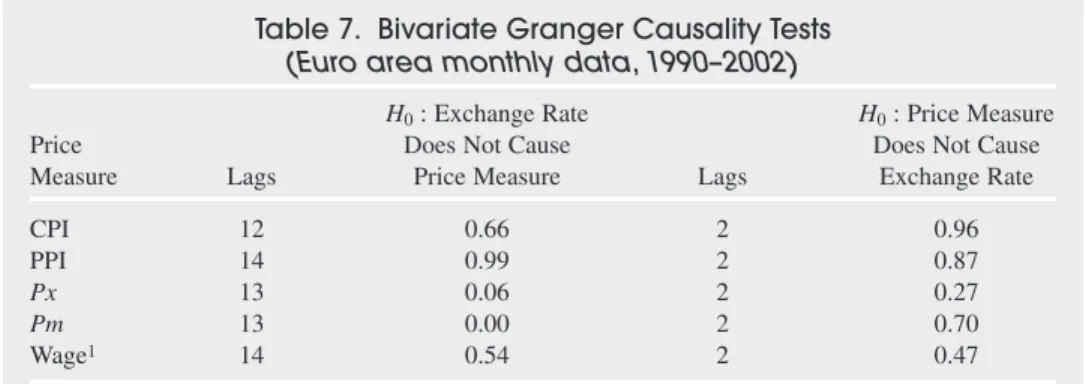
Granger causality tests were conducted to examine whether changes in euro area exchange rates and prices have predictive content for each other. Simple bivariate tests indicate that the nomi-nal effective exchange rate Granger-causes (i.e., helps predict) several price measures, but prices fail to Granger-cause exchange rates. The exchange rate is found to be a significant pre-dictor for trade prices and has predictive content for wages at shorter lag length (see Table 7).
Block Exogeneity Tests
To generalize Granger causality tests to a multivariate context, consider the following parti-tioned VAR(p) system:
Table 6. Co-Integration Tests
(Euro area monthly data, 1990–2002)
Number of Regressors PˆzTest (demeaned) PˆzTest (demeaned and detrended)
n =5 115.10 120.43
(225.23) (284.01)
Source: IMF staff estimates.
Notes: Multivariate trace statistic based on Phillips and Ouliaris (1990); 10 percent critical value given in parentheses.
Table 7. Bivariate Granger Causality Tests
(Euro area monthly data, 1990–2002)
H0: Exchange Rate H0: Price Measure
Price Does Not Cause Does Not Cause
Measure Lags Price Measure Lags Exchange Rate
CPI 12 0.66 2 0.96
PPI 14 0.99 2 0.87
Px 13 0.06 2 0.27
Pm 13 0.00 2 0.70
Wage1 14 0.54 2 0.47
Source: IMF staff estimates.
Notes: Reported numbers are p-values on the relevant exclusion restriction (F-test). Lag length selection based on Akaike Information Criterion.
where c1and c2represent a constant term and monthly time dummies, Prepresents the (5 ×1)
vector of price variables, X1and X2 are (p × 1) and (5p ×1) vectors of lagged changes in
exchange rates and prices, respectively, with conformable matrices of autoregressive coeffi-cients A1, A2, B1, and B2. Block exogeneity test results are shown in Table 8.
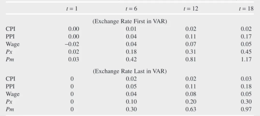
Sensitivity Analysis
As seen in Table 9, the implied pass-through elasticities from the two VARs (i.e., with the exchange rate first and last in the ordering) are fairly similar. On impact, euro area prices are essentially predetermined in response to the exchange rate shock in the two VARs. It should be stressed, however, that the exchange rate shock has zero contemporaneous effect on prices (i.e., prices are exactly predetermined) by constructionin the latter VAR, based on the ordering of
∆ ∆ s c A X A X P c B X B X t t t t t t t = + + + = + + + 1 1 1 2 2 1 2 1 1 2 2 2 ε εtt ,
Table 8. Block Exogeneity Tests
(Euro area monthly data, 1990–2002)
Lag Length H0: A2=0 H0: B1=0
p=7 32.42 50.48
(0.59) (0.04)
Source: IMF staff estimates.
Notes: Test statistic is based on likelihood ratio test with degrees of freedom correction and is distributed as χ2(5p). Significance levels are given in parentheses.
Table 9. Euro Area Pass-Through Elasticities Across VAR Reorderings
t=1 t=6 t=12 t=18
(Exchange Rate First in VAR)
CPI 0.00 0.01 0.02 0.02
PPI 0.00 0.04 0.11 0.17
Wage −0.02 0.04 0.07 0.05
Px 0.02 0.18 0.31 0.45
Pm 0.03 0.42 0.81 1.17
(Exchange Rate Last in VAR)
CPI 0 0.02 0.02 0.03
PPI 0 0.05 0.11 0.18
Wage 0 0.04 0.08 0.05
Px 0 0.10 0.20 0.30
Pm 0 0.30 0.63 0.97
Source: IMF staff estimates.
Notes: Entries report percent change in price measure divided by percent change in exchange rate in response to unit exchange rate shock from Cholesky decomposition of innovations.
variables. In the case of the euro area (and the United States) this restriction appears valid empirically. Hence, the reordering makes little difference. For other industrial countries, how-ever, this is generally not true for trade prices, as shown by Table 2, and should thus not be imposed a priori. So long as the exchange rate appears beforetrade prices in the VAR for these countries, alternative impulse-response functions will closely match those reported in the text.
REFERENCES
Anderton, Robert, 2003, “Extra-Euro Area Manufacturing Import Prices and Exchange Rate Pass-Through,” ECB Working Paper No. 219 (Frankfurt: European Central Bank). Bekx, Peter, 1998, “The Implications of the Introduction of the Euro for Non-EU Countries,”
Euro Papers 26 (Brussels: European Commission).
Bergin, Paul, and Robert C. Feenstra, 2001, “Pricing-to-Market, Staggered Contracts, and Real Exchange Rate Persistence,” Journal of International Economics,Vol. 54 (August), pp. 333–59.
Betts, Caroline, and Michael B. Devereux, 1996, “The Exchange Rate in a Model of Pricing-to-Market,” European Economic Review,Vol. 40 (April), pp. 1007–21.
———, 2000, “Exchange Rate Dynamics in a Model of Pricing-to-Market,” Journal of International Economics,Vol. 50 (February), pp. 215–44.
Burstein, Ariel T., João C. Neves, and Sergio Rebelo, 2003, “Distribution Costs and Real Exchange Rate Dynamics During Exchange-Rate-Based Stabilizations,” Journal of Monetary Economics,Vol. 50 (September), pp. 1189–214.
Calvo, Guillermo, A., 1983, “Staggered Prices in a Utility-Maximizing Framework,” Journal of Monetary Economics,Vol. 12 (September), pp. 383–98.
Campa, Jose M., and Linda S. Goldberg, 2002, “Exchange Rate Pass-Through into Import Prices: A Macro or Micro Phenomenon?” Staff Reports No. 149 (New York: Federal Reserve Bank of New York).
Cheung, Y., M. Chinn, and A. Pascual, 2002, “Empirical Exchange Rate Models of the Nineties: Are Any Fit to Survive?” NBER Working Paper No. 9393 (Cambridge, Massachusetts: National Bureau of Economic Research).
Choudhri, Ehsan U., Hamid Faruqee, and Dalia S. Hakura, 2002, “Explaining the Exchange Rate Pass-Through in Different Prices,” IMF Working Paper 02/224 (Washington: International Monetary Fund).
———, 2005, “Explaining the Exchange Rate Pass-Through in Different Prices,” Journal of International Economics,Vol. 65 (March), pp. 349–74.
Choudhri, Ehsan U., and Dalia S. Hakura, 2001, “Exchange Rate Pass-Through to Domestic Prices: Does the Inflationary Environment Matter?” IMF Working Paper 01/194 (Washington: International Monetary Fund).
Corsetti, Giancarlo, and Luca Dedola, 2002, “Macroeconomics of International Price Discrimination,” ECB Working Paper No. 176 (Frankfurt: European Central Bank). Corsetti, Giancarlo, and Paolo Pesenti, 2002, “Self-Validating Optimum Currency Areas,”
NBER Working Paper No. 8783 (Cambridge, Massachusetts: National Bureau of Economic Research).
Devereux, Michael, and Charles Engel, 2002, “Exchange Rate Pass-Through, Exchange Rate Volatility, and Exchange Rate Disconnect,” Journal of Monetary Economics,Vol. 49 (July), pp. 913–40.
———, 2003, “Monetary Policy in the Open Economy Revisited: Price Setting and Exchange-Rate Flexibility,” Review of Economic Studies,Vol. 70 (4), pp. 765–83.
———, and Cedric Tille, 1999, “Exchange Rate Pass-Through and the Welfare Effects of the Euro,” NBER Working Paper No. 7382 (Cambridge, Massachusetts: National Bureau of Economic Research).
Dominguez, Kathryn, 1999, “The Role of the Yen,” in International Capital Flows, ed. by Martin Feldstein (Chicago: University of Chicago Press), pp. 133–71.
Engel, Charles, 2002, “Expenditure Switching and Exchange Rate Policy,” in NBER Macroeconomics Annual 2002, ed. by Mark Gertler and Kenneth Rogoff (Cambridge, Massachusetts: MIT Press).
Faruqee, Hamid, 1995, “Pricing to Market and the Real Exchange Rate,” IMF Staff Papers,
Vol. 42 (December), pp. 855–81.
———, 2003, “Exchange Rate Pass-Through and External Adjustment in the Euro Area,” in
Euro Area Policies, Selected Issues, IMF Country Report No. 03/298 (Washington: International Monetary Fund).
Flath, David, 2003, “Regulation, Distribution Efficiency, and Retail Density,” NBER Working Paper No. 9450 (Cambridge, Massachusetts: National Bureau of Economic Research). Flood, Robert P., and Andrew K. Rose, 1995, “Fixing Exchange Rates, A Virtual Quest for
Fundamentals,” Journal of Monetary Economics,Vol. 36 (August), pp. 3–37.
Gagnon, Joseph, and Jane Ihrig, 2001, “Monetary Policy and Exchange Rate Pass-Through,” International Finance Discussion Papers No. 704 (revised March 2002) (Washington: Board of Governors of the Federal Reserve System).
Giovannini, Alberto, 1988, “Exchange Rates and Traded Goods Prices,” Journal of International Economics,Vol. 24 (February), pp. 45–68.
Goldberg, Penelopi, and Michael Knetter, 1997, “Goods Prices and Exchange Rates: What Have We Learned?” Journal of Economic Literature,Vol. 35 (September), pp. 1243–72. Hahn, Elke, 2003, “Pass-Through of External Shocks to Euro Area Inflation,” ECB Working
Paper No. 243 (Frankfurt: European Central Bank).
Hamilton, James D., 1994, Time Series Analysis(Princeton, New Jersey: Princeton University Press).
Herzberg, Valerie, George Kapetanios, and Simon Price, 2003, “Import Prices and Exchange Rate Pass-Through: Theory and Evidence from the United Kingdom,” Bank of England Working Paper No. 182 (London: Bank of England).
Hüfner, Felix P., and Michael Schroder, 2002, “Exchange Rate Pass-Through to Consumer Prices: A European Perspective,” Center for European Economic Research Discussion Paper 02-20 (Mannheim, Germany: Center for European Economic Research).
Isard, Peter, Hamid Faruqee, G. Russell Kincaid, and Martin Fetherston, 2001, Methodology for Current Account and Exchange Rate Assessments, IMF Occasional Paper No. 209 (Washington: International Monetary Fund).
Jeanne, Olivier, and Andrew K. Rose, 2002, “Noise Trading and Exchange Rate Regimes,”
Quarterly Journal of Economics,Vol. 117 (May), pp. 537–69.
Kasa, Kenneth, 1992, “Adjustment Costs and Pricing-to-Market Theory and Evidence,” Journal of International Economics,Vol. 32 (February), pp. 1–30.
Kieler, Mads, 2001, “Tracking the Pass-Through of External Shocks to Euro Area Inflation,” in
Monetary and Exchange Rate Policies of the Euro Area—Selected Issues,prepared by A. Jaeger, K. Ross, Z. Kontolemis, M. Kieler, and G. Meredith, IMF Country Report No. 01/201 (Washington: International Monetary Fund), pp. 52–67.
Kollmann, Robert, 2001, “The Exchange Rate in a Dynamic-Optimizing Business Cycle Model with Nominal Rigidities: A Quantitative Investigation,” Journal of International Economics,