Evaluation and Comparison of 3D Intervertebral Disc
Localization and Segmentation Methods for 3D T2 MR
Data: A Grand Challenge
Guoyan Zhenga,∗,
Chengwen Chua, Daniel L. Belav´yb,c, Bulat Ibragimovd,e, Robert Korezd, Tomaˇz Vrtovecd, Hugo Huttf, Richard Eversonf, Judith Meakinf,
Isabel L˘opez Andradeg, Ben Glockerg, Hao Chenh, Qi Douh, Pheng-Ann Hengh, Chunliang Wangi, Daniel Forsbergi,j, Aleˇs Neubertk, Jurgen Frippl, Martin Urschlerm, Darko Sternn, Maria Wimmero, Alexey A.
Novikovo, Hui Chenga, Gabriele Armbrechtc, Dieter Felsenbergc, Shuo Lip
aInstitute for Surgical Technology and Biomechanics, University of Bern, Switzerland bInstitute of Physical Activity and Nutrition Research, Deakin University, Burwood,
Victoria, Australia
cCharit´eUniversity Medical School Berlin, Germany dUniversity of Ljubljana, Slovenia
eStanford University, USA
fUniversity of Exeter, The United Kingdom gImperial College London, The United Kingdom
hThe Chinese University of HongKong, China iSectra, Linko¨ping, Sweden
jCase Western Reserve University and University Hospitals Case Medical Center, USA kUniversity of Queensland, Australia
lThe Australian e-Health Research Centre, CSIRO Health and Biosecurity, Australia mGraz University of Technology, Austria
nLudwig Boltzmann Institute for Clinical Forensic Imaging, Austria oVRVis Center for Virtual Reality and Visualization, Austria
pUniversity of Western Ontario, Canada
Abstract
The evaluation of changes in Intervertebral Discs (IVDs) with 3D Magnetic Resonance (MR) Imaging (MRI) can be of interest for many clinical
applica-∗Corresponding author. Tel.: +41-31-6315956 (Guoyan Zheng)
Email address: [email protected], [email protected] (Guoyan Zheng)
tions. This paper presents the evaluation of both IVD localization and IVD segmentation methods submitted to the Automatic 3D MRI IVD Localiza-tion and SegmentaLocaliza-tion challenge, held at the 2015 InternaLocaliza-tional Conference on Medical Image Computing and Computer Assisted Intervention (MIC-CAI2015) with an on-site competition. With the construction of a manually annotated reference data set composed of 25 3D T2-weighted MR images acquired from two different studies and the establishment of a standard val-idation framework, quantitative evaluation was performed to compare the results of methods submitted to the challenge. Experimental results show that overall the best localization method achieves a mean localization dis-tance of 0.82mm and the best segmentation method achieves a mean Dice of 91.8%, a mean average absolute distance of 1.08mm and a mean Haus-dorff distance of 4.34mm, respectively. The strengths and drawbacks of each method are discussed, which provides insights into the performance of differ-ent IVD localization and segmdiffer-entation methods.
Keywords: Intervertebral disc, MRI, Localization, Segmentation, Challenge, Evaluation
1. Introduction
Low back pain (LBP) is one of the most prevalent health problems amongst the world’s population and is a leading cause of disability that affects work performances and well-being (Maniadakis and Gray, 2000; Andersson, 2011; Wieser et al., 2011). A strong association between LBP and intervertebral disc (IVD) degeneration has been repeatedly reported in various clinical stud-ies (Luoma et al., 2000; Kjaer et al., 2005; Cheung et al., 2009). Although almost every medical imaging modality has been used to evaluate lumbar de-generative disc disease, Magnetic Resonance (MR) Imaging (MRI) is widely recognized as the imaging technique of choice for the assessment of lumbar IVD abnormalities due to its excellent soft tissue contrast and no ionizing radiation (Emch and Modic, 2011; Parizel et al., 2007). This, in turn, has sparked specific interest in developing methods for automated image analy-sis and quantification for the diagnoanaly-sis of spinal diseases using MR images, though most of them work only with two-dimensional (2D) images. Here the term image analysis refers to localization and segmentation of the IVDs, which is a step prior to the quantification process. The published methods can be roughly classified into two groups: disc detection and disc
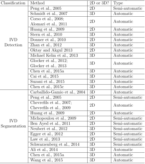
segmen-tation. Table 1 shows a summary of the state-of-the-art methods for IVD detection and segmentation.
The methods in the first group focus on automated detection of the discs or vertebrae but without segmenting them (Peng et al., 2005; Schmidt et al., 2007; Corso et al., 2008; Alomari et al., 2011; Stern et al., 2010; Donner et al., 2010; Oktay and Akgul, 2013). For example, Peng et al. (2005) used intensity profiles to localize the 24 articulated vertebrae from whole spine MR images and their method required a manual selection of the so-called best MR image slice among all the sagittal slices. Schmidt et al. (2007) proposed a part-based graphical model for spine detection and labeling. They used the part-based graphical model to represent both the appearance of local parts and the shape of the anatomy in terms of geometric relations between parts. Features for detecting parts were learned from a set of training data in manually marked image regions. Along the same line, Alomari et al. (Corso et al., 2008; Alomari et al., 2011) presented a different graphical model for the lumbar disc localization. They used a two-level probabilistic model with latent variables to capture both pixel- and object-level features. Generalized expectation maximization method was used for optimization. The method was validated on 2D sagittal MR images. Stern et al. (2010) described another method for automatic IVD detection from MR images of lumbar spine. Their method worked by first extracting spinal centerlines and then detecting the centers of vertebral bodies and IVDs by analyzing the image intensity and gradient magnitude profiles extracted along the spinal centreline. There also exist methods using Markov Random Field (MRF)-based inference. Donner et al. (2010) proposed to formulate the localization of an object model from an input image as an MRF-based optimal labeling problem. They used MRF to encode the relation between the model and the entire search image. Recently, Oktay and Akgul (2013) described a method to simultaneously localize lumbar vertebrae and IVDs from 2D sagittal MR images using support vector machine (SVM) based MRF.
In contrast, the methods in the second group aim for disc segmenta-tion. The disc detection in these methods could be done manually, semi-automatically or fully-semi-automatically. Chevrefils et al. (2007, 2009) presented a texture analysis based method for automatic segmentation of IVDs from 2D MR images of scoliotic spines. Their method exploited a combination of sta-tistical and spectral texture features to discriminate closed regions represent-ing IVDs from background in MR images. The closed regions are obtained with the watershed approach. Michopoulou et al. (2009) proposed a
prob-Table 1: Summary of the state-of-the-art methods for IVD detection and segmentation.
Classification Method 2D or 3D? Type
IVD Detection
Peng et al., 2005 2D Semi-automatic
Schmidt et al., 2007 3D Automatic
Corso et al., 2008;
Alomari et al., 2011 2D Automatic
Huang et al., 2009 2D Automatic
Stern et al., 2010 3D Automatic
Donner et al., 2010 2D Automatic
Zhan et al., 2012 3D Automatic
Oktay and Akgul 2013 2D Automatic
Michael Kelm et al., 2013 3D Automatic
Glocker et al., 2012;
Glocker et al., 2013 3D Automatic
Chen et al., 2015a 3D Automatic
Cai et al., 2015 3D Automatic
Suzani et al., 2015 3D Automatic
Chen et al., 2015c 3D Automatic
IVD Segmentation
Carballido-Gamio et al., 2004 3D Automatic
Peng et al., 2005 2D Semi-automatic
Chevrefils et al., 2007;
Chevrefils et al., 2009 2D Automatic
Huang et al., 2009 2D Automatic
Michopoulou et al., 2009 2D Semi-automatic
Ben Ayed et al., 2011 2D Semi-automatic
Neubert et al., 2012 3D Semi-automatic
Egger et al., 2012 2D Semi-automatic
Law et al., 2013 2D Semi-automatic
Schwarzenberg et al., 2014 3D Semi-automatic
Ali et al., 2014 3D Automatic
Chen et al., 2015a 3D Automatic
abilistic atlas-based method for segmentation of degenerated lumbar IVDs from 2D MR images of the spine. Their method was semi-automatic and re-quired an interactive selection of the leftmost and rightmost disc points. The reported Dice coefficents of this method were 91.6% for normal and 87.2% for degenerated discs. A statistical shape models-based method was proposed by Neubert et al. (2012) for automated three-dimensional (3D) segmentation of high resolution spine MR images. Their method required an interactive placement of a set of initial rectangles along spine curve. Different types of graph theory based methods (Carballido-Gamio et al., 2004; Huang et al., 2009; Ali et al., 2014; Ben Ayed et al., 2011; Egger et al., 2012; Yao et al., 2006; Schwarzenberg et al., 2014) are also popular in disc or vertebra segmen-tation. Among the methods in this category, there exist methods in the form of normalized cut (Carballido-Gamio et al., 2004; Huang et al., 2009). For example, Carballido-Gamio et al. (2004) applied the normalized cut to seg-ment T1-weighted MR images. Huang et al. (2009) improved this method by proposing an iterative algorithm and evaluated their method on 2D sagittal MR slices. There also exist graph theory based methods in the form of graph cut (Ali et al., 2014; Ben Ayed et al., 2011). For example, Ben Ayed et al. (2011) designed new object-interaction priors for graph cut image segmen-tation and applied their method to IVD delineation in 2D MR lumbar spine images. Their method required a manual selection of the first disc center. Evaluated on 15 2D mid-sagittal MR slices, this method achieved an average 2D Dice overlap coefficent of 85%. More recently, following the idea intro-duced by Li et al. (2006), both square-cut (Egger et al., 2012) and cubic-cut
(Schwarzenberg et al., 2014) methods were proposed. Thesquare-cut method works only on 2D sagittal slices of MR data while the cubic-cut method can be used for 3D spinal MR image segmentation. Another method on IVD segmentation from middle sagittal spine MR images was introduced by Law et al. (2013). They used the anisotropic oriented flux detection scheme to distinguish the discs from the neighboring structures with similar intensity with a minimal user interaction.
Recently, machine learning-based methods have gained more and more interest in the medical image analysis community. Most of these methods are based on ensemble learning principles that can aggregate predictions of multiple classifiers and demonstrate superior performance in various chal-lenging medical image analysis problems. For example, Zheng et al. (2008) proposed marginal space learning to automatically localize the heart cham-ber from 3D Computed Tomography (CT) data. This method has been
successfully used for spine detection in CT and MR images (Michael Kelm et al., 2013). Zhan et al. (2012) presented a hierarchical strategy and local articulated model to detect vertebrae and discs from 3D MR images. They used a Haar filter based Adaboost classifier and a local articulated model for calculating the spatial relations between vertebrae and discs. A combi-nation of wavelet transform based Adaboost classifier and iterative normal-ized cut was proposed by Huang et al. (2009) for detecting and segmenting vertebrae. Due to the successful applications of Random Forest (RF) regres-sion for automatic localization of organs from 3D volumetric CT/MR data (Pauly et al., 2011; Criminisi et al., 2013), such a technique has been used by Glocker et al. (2012, 2013) for localization and identification of vertebrae in arbitrary field-of-view CT scans. Another two regression-based approaches were introduced by Chen et al. (2015a) and Wang et al. (2015), respectively. More specifically, Chen et al. (2015a) proposed a unified data-driven regres-sion and classification framework to tackle the problem of localization and segmentation of IVDs from T2-weighted MR data while Wang et al. (2015) proposed to address the segmentation of multiple anatomic structures in mul-tiple anatomical planes from mulmul-tiple imaging modalities with a sparse kernel machines-based regression. More recently, the advancement of deep learn-ing approaches provides another course of efficient methods for spinal image processing. For example, Cai et al. (2015) proposed to use a 3D deformable hierarchical model for multi-modality vertebra recognition in arbitrary view where multi-modal features extracted from deep networks were used for ver-tebra landmark detection. While both Chen et al. (2015c) and Suzani et al. (2015) used deep learning approaches for automatic vertebrae detection and localization from spinal CT data, they used different types of deep neural networks. More specifically, the work done by Suzani et al. (2015) was based on feed-forward neural networks while the work done by Chen et al. (2015c) was based on deep convolutional neural networks.
Meaningful comparisons of algorithm performance among various state-of-the-art IVD localization and segmentation methods are highly desired. However, direct and objective comparisons are difficult to achieve due to fol-lowing two issues: 1) Different MR data sets acquired with different image acquisition protocols are used in different studies, and most of these MR data sets are not publicly available. Although there exists one open data set for comparing algorithms for clinical vertebral segmentation from 3D CT data (Yao et al., 2016), to the best of our knowledge, there exists only one open MR data set with the associated manual delineation of IVDs (Oktay and
Akgul, 2013). This open MR data set, however, cannot be used to evalu-ate and compare 3D IVD localization and segmentation algorithms, as only 2D mid-sagittal slices are available in the data set; and 2) Different evalu-ation metrics are used in different studies, which precludes the possibility of direct comparison. Therefore, to address the above mentioned challenges in algorithm comparison, it is necessary to establish a standard validation framework with a publicly available reference MR data set. To reach this goal, a grand challenge on Automatic IVD Localization and Segmentation from 3D T2 MR Data was held in conjunction with the third MICCAI Work-shop on Computational Methods and Clinical Applications for Spine Imaging (CSI) (http://ijoint.istb.unibe.ch/challenge/index.html).
The challenge report described in this paper intends to first construct an annotated reference data set composed of 3D T2-weighted Turbo Spin Echo (TSE) MR images for validation purpose and then to establish a standard framework for an objective comparison of different IVD localization and seg-mentation algorithms. Details of challenge setup and challenge results will be described in the following sections. More specifically, in Section 2, challenge organization, the established validation framework, the data sets used within the challenge and the participation teams will be introduced. In Section 3, summary about each submitted algorithm will be described. The validation results for all submitted algorithms will be described in Section 4. Discus-sions of the performance and the computational efficiency of methods of all participating teams will be presented in Section 5, followed by conclusion in Section 6.
2. Challenge Setup 2.1. Organization
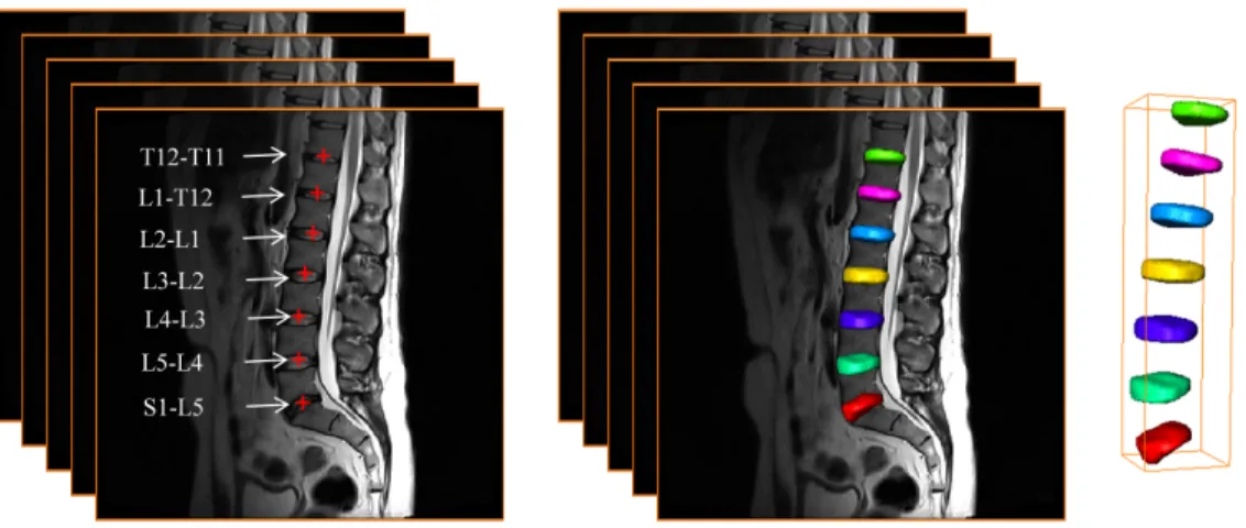
The aim of the challenge is to investigate (semi-)automatic IVD local-ization and segmentation algorithms and to provide a standard evaluation framework with a set of 3D T2-weighted TSE MR images. There are 7 IVDs T11-S1 to be localized and segmented from each image as shown in Fig. 1. Thus, the challenge has been divided into two parts: the localization part and the segmentation part. In the localization part, the task is to fully au-tomatically identify the centers of 7 IVDs T11-S1 from each image. In the segmentation part, the task is to automatically segment 7 IVD regions T11 S1 from each image. Each team can choose to participate in either one of the two parts or in both parts.
Figure 1: The 7 IVDs to be localized and segmented from each image.
There are two stages in the challenge. In stage 1, a training data set and the associated ground truth were released on March 1st, 2015 for method development and a first test data set were released on August 15, 2015 for method testing. In stage 2, an on-site competition was organized for which a second test data set was released on October 05, 2015.
2.2. Validation framework
The established validation framework includes five standard metrics to evaluate the algorithm performance, two for localization and three for seg-mentation. For evaluation of the localization performance, we propose to use the following two metrics:
1. Mean localization distance (MLD) with standard deviation (SD)
We first compute the localization distance Rfor each IVD center using
R =p(∆x)2+ (∆y)2+ (∆z)2 (1)
where ∆x, ∆y, and ∆zare respectivelyx,y, andzcoordinate difference between the identified IVD center and the ground truth (GT) IVD center calculated from the ground truth segmentation.
MLD and SD are then defined as follows: M LD = PNimages i=1 PNIV Ds j=1 Rij NimagesNIV Ds SD = r PNimages i=1 PNIV Ds j=1 (Rij−M LD) 2 NimagesNIV Ds (2)
where Nimages is the number of MR images, and NIV Ds is the number
of IVDs.
2. Successful detection rate (SDR) with various ranges of accu-racy
If the distance between the localized IVD center and the ground truth center is no greater than t mm, the localization of this IVD is con-sidered as a successful detection; otherwise, it is concon-sidered as a false localization. The successful localization rate Pt with accuracy of less
than t mm is formulated as follows Pt =
number of accurate IVD localizations
number of IVDs ×100% (3)
For evaluating the segmentation performance, we use the following three metrics:
1. Dice overlap coefficients (Dice): Dice measures the percentage of correctly segmented voxels. Dice (Dice, 1945) is computed by
Dice = 2|A∩B|
|A|+|B| ×100% (4)
whereAis the set of foreground voxels in the ground-truth data andB is the corresponding set of foreground voxels in the segmentation result, respectively. Larger Dice metric means better segmentation accuracy. 2. Average absolute distance (AAD): AAD measures the average
absolute distance from the ground truth IVD surface and the auto-matically segmented surface. To compute the AAD, we first generate a surface mesh from binary IVD segmentation. For each vertex on the surface model derived from the automatic segmentation, we find its closest distance to the surface model derived from the associated ground-truth segmentation. The AAD is then computed as the average of distances of all vertices. Smaller AAD means better segmentation accuracy.
Table 2: Demographic statistics of the 25 subjects.
Subject Characteristics Mean ± SD Min Max
Age (year) 34.4 ± 8.1 20 45
Weight (kg) 76.1 ± 10.7 59 104
Height (cm) 179.5 ± 6.9 169.0 196.1
3. Hausdorff distance (HD): HD measures the Hausdorff distance (Hut-tenlocher et al., 1993) between the ground truth IVD surface and the segmented surface. To compute the HD, we use the same surface models as we used for computing the AAD. Smaller HD means better segmen-tation accuracy.
2.3. Description of Image Data Sets
There are 25 3D T2-weighted TSE MR images collected from 25 male subjects in two different studies investigating IVD morphology change af-ter prolonged bed rest (spaceflight simulation) (Belavy et al., 2012, 2011). Table 2 summarizes the demographic statistics of the 25 subjects. Each sub-ject was scanned with 1.5 Tesla MR scanner of Siemens Magnetom Sonata (Siemens Healthcare, Erlangen, Germany) with following protocol to gener-ate T2-weighted sagittal images: repetition time of 5240 ms and echo time of 101 ms were used in acquisition of 15 3D T2-weighted MR images in the first study while repetition time of 6220 ms and echo time of 105 ms were used in acquisition of the rest 10 3D T2-weighted MR images in the second study. The resolution of all images were resampled to 2mm × 1.25mm × 1.25mm. Each image contains at least 7 IVDs T11-S1. Thus, in this challenge, we only consider 7 IVDs T11-S1. An ethical approval was obtained from the Eth-ical Committee of the Charit´e University Medical School Berlin, Germany, to conduct the study. These 25 MR images were divided into three subsets as Training data (ten 3D T2-weighted MR images from the first study plus five 3D T2-weighted MR images from the second study), Test1 data (four 3D T2-weighted MR images from the first study and one 3D T2-weighted MR image from the second study) and Test2 data (one 3D T2-weighted MR image from the first study and four 3D T2-weighted MR images from the second study) for the challenge with two stages.
For each one of these 3D T2-weighted MR images, the segmentation of 7 IVDs T11-S1 was conducted in two stages. In the first stage, slice by slice
Table 3: Inter-observer variability of manual segmentation generated by three trained raters and an experienced expert using the metrics defined in Section 2.2.
MLD
±
SD (mm)
Mean Dice
±
SD (%)
Mean AAD
±
SD (mm)
0.16
±
0.17
99.1
±
0.7
0.81
±
0.09
manual segmentation was performed by three trained raters with different degrees of expertise (3 - 15 years of experience with MR/CT segmentation) using Amira software (http://www.vsg3d.com/amira) under the guidance of clinicians. The reference segmentation for each MR image was then gener-ated based on consensus reading of all three raters, e.g., the majority voting of all three manual segmentations. In the second stage, an experienced sur-geon was asked to independently segment all the 25 MR images using also the Amira software to generate another set of segmentation.
We then evaluated the inter-observer variability for the two sets of manual segmentations to assess the consistency and variability. The inter-observer variability was calculated using the metrics defined in Section 2.2 and pre-sented in Table 3. The results show that the reference segmentation has high consistency with the expert segmentation and thus we use the reference segmentation as the associated ground-truth for evaluating performance of different algorithms submitted to the challenge. The ground-truth IVD cen-ters were then calculated as centroids of the associated IVD regions.
2.4. Participating teams
A total of 16 teams (from 11 countries) from both industry and academy registered in this challenge, and initially 10 teams submitted their results on the Test1 data. All these 10 teams were invited to participate the on-site competition in stage 2. Afterwards, we received agreements from 9 teams to include their results in this paper. The name abbreviation for each included team and the title of their contribution are given as follows. To simplify the description below, we will use the team abbreviations to refer both the teams and the methods introduced by the associated teams.
1. ICL: Lopez Andrade and Glocker (Lopez Andrade and Glocker, 2015). Complementary classification forests with graph-cut refinement for ac-curate intervertebral disc localisation and segmentation (UK).
2. Sectra: Wang and Forsberg (Wang and Forsberg, 2015). Segmen-tation of intervertebral discs in 3D MR data using multi-atlas based registration (Sweden).
3. UNIBE: Chu et al. (Chu et al., 2015). Localization and segmentation of 3D intervertebral discs from MR images via a learning based method (Switzerland).
4. UNICHK: Chen et al. (Chen et al., 2015b). DeepSeg: Deep segmen-tation networks for intervertebral disc localization and segmensegmen-tation (China).
5. UNIEXE: Hutt et al. (Hutt et al., 2015). 3D intervertebral disc segmentation from MR using supervoxel-based Conditional Random Fields (CRFs) (UK).
6. UNIGRA Urschler et al., (Urschler et al., 2015). Automatic interver-tebral disc localization and segmentation in 3D MR images based on regression forests and active contours (Austria).
7. UNILJU: Korez et al. (Korez et al., 2015a). Deformable model-based segmentation of intervertebral discs from MR spine images by using the SSC descriptor (Slovenia).
8. UNIQUE: Neubert et al. (Neubert et al., 2015). Automated inter-vertebral disc segmentation using probabilistic shape estimation and active shape models (Australia).
9. VRVIS: Wimmer and Novikov. A machine learning based pipeline for automated intervertebral disc labeling and segmentation in 3D T2-weighted MR data (Austria).
3. Methods
In this section, we would like to present the methods that were submitted to the challenge. In the next section we will analyze the experimental results achieved by these methods.
3.1. Method of team ICL
Lopez Andrade and Glocker (2015) proposed a pipeline for the task of automatic localization and segmentation of IVDs in the lumbar spine involv-ing a combination of several machine learninvolv-ing techniques. The spine detec-tion phase aims to estimate the dimensions and locadetec-tion of a 3D bounding box that contains the spine and makes use of two complementary RFs (see (Glocker et al., 2016) for details) that classify voxels based on Histogram of Oriented Gradients (HOG) and Haar-like features, respectively. The disc probability maps generated by the classification are then processed by the
Density Based Spatial Clustering of Applications with Noise algorithm (DB-SCAN) (Ester et al., 1996), which outputs the central points corresponding to high density areas. An outlier removal stage discards the false disc centroids. The segmentation is posed as an energy minimization problem solved via graph-cuts (see Boykov and Funka-Lea (2006)). Each of the discs in the image is segmented separately, and the result is then combined into a single label map. The designed graph has two types of edges: terminal edges, that connect the voxels and the terminal nodes s and t; and non-terminal edges, that connect neighbouring voxels. The capacities of the edges between neighbouring voxels are defined by the following equation; where dist(vi, vj)
is the Euclidean distance between the voxels vi and vj,IF(vi) is the intensity
of voxel vi in the filtered image, σ2 is an estimation of the noise variance, k
is a constant that normalizes the edge capacities between 0 and 100, and λ corresponds to the relative importance of non-terminal and terminal edges. σ2 is estimated for the input filtered image as the difference between this image and the same image after applying a discrete Gaussian filtering.
N(Li, Lj) =λ h k dist(vi, vj) exp −(IF(vi)−IF(vj))2 2σ2 i (5) The capacities of the terminal edges are further modulated by the prob-ability label maps. The minimization problem is then solved via the max-flow/min-cut algorithm. Isolated regions whose area is smaller than 50mm2 are discarded. Similarly, if there are several connected objects, the ones whose area is smaller than the mean area of all the objects are also deleted.
3.2. Method of team Sectra
Building upon two earlier works, with one for vertebral body detection and labeling in MR data (Lootus et al., 2015) and the other for multi-atlas based segmentation of vertebrae in CT data (Forsberg, 2015), Wang and Forsberg (2015) propose an approach for the task of localization and segmentation of IVDs in MR data. In the first step, vertebral bodies are detected and labeled using integral channel features and a graphical parts model. The second step consists of image registration, where a set of image volumes with corresponding IVD atlases are registered to the target volume using the output from the first step as initialization for the registration. In the final step, the registered atlases are combined using label fusion to derive the combined localization and segmentation of the IVDs.
3.3. Method of team UNIBE
Building upon the work introduced by Chen et al. (2015a), Chu et al. (2015) develop a two-stage coarse-to-fine approach to tackle the problems of fully automatic localization and segmentation of 3D IVD from MR images. More specifically, in the first stage, the learning-based, unified data-driven regression and classification framework introduced by Chen et al. (2015a) is used to roughly localize and segment each disc. The localization of 3D IVD is solved with a data-driven regression where they aggregated the votes from a set of randomly sampled image patches to get a probability map of the location of a target vertebral body in a given image. The resultant proba-bility map is then further regularized by Hidden Markov Model (HMM) to eliminate potential ambiguity caused by the neighboring discs. The output from the localization allows one to define a region of interest (ROI) for the segmentation step, where a data-driven classification is used to estimate the likelihood of a pixel in the ROI being foreground or background. The es-timated likelihood is combined with the prior probability, which is learned from a set of training data, to get the posterior probability of the pixel. The coarse segmentation of the target IVD is then done by a binary thresholding on the estimated probability. In the second stage, after the IVDs are roughly segmented, a multi-atlas fusion based graph cut method is used to modify the coarse segmentation of each IVD. A registration framework is developed which allows not only accurate alignment of multiple atlases within the tar-get image space but also a fast selection of atlas for generating probabilistic atlas (PA). The generated PAs is finally used in a graph cut method (Boykov and Funka-Lea, 2006) to get the refined segmentation of IVDs.
3.4. Method of team UNICHK
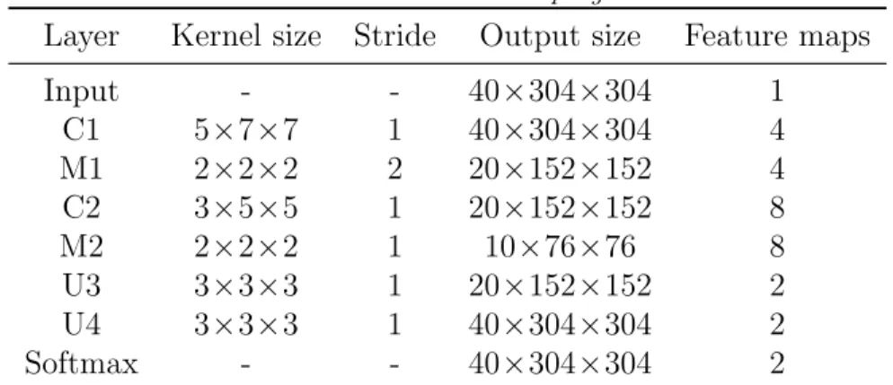
Chen et al. (2015b) propose a deeply supervised segmentation network called DeepSeg-3D for automatic IVD localization and segmentation from MR images.DeepSeg-3D takes full advantage of volumetric information based on 3D convolutional kernels and makes full use of volumetric information in all dimensions for better discrimination performance. They implement the convolutional network in a 3D format, which inputs 3D volumetric data and directly outputs a 3D prediction mask. Specifically, the architecture of neu-ral network contains 2 convolutional layers, 2 max-pooling layer for down-sampling and 2 unpooling layers for up-down-sampling. Three architectures with different convolutional kernel sizes are used. The details of one architecture of DeepSeg-3D can be seen in Table. 4. Finally, a softmax classification layer
Table 4: The architecture ofDeepSeg-3D model
Layer Kernel size Stride Output size Feature maps
Input - - 40×304×304 1 C1 5×7×7 1 40×304×304 4 M1 2×2×2 2 20×152×152 4 C2 3×5×5 1 20×152×152 8 M2 2×2×2 1 10×76×76 8 U3 3×3×3 1 20×152×152 2 U4 3×3×3 1 40×304×304 2 Softmax - - 40×304×304 2
C: convolution, M: max-pooling, U: unpooling
is followed to generate the prediction probabilities. All the convolutional ker-nels of theDeepSeg-3D model were initialized from the Gaussian distribution and the input to the network is the direct 3D volumetric data. The model was trained by minimizing the cross-entropy loss via standard back-propagation. The output fromDeepSeg-3D is further processed with thresholding and disk filtering to generate local smooth maps. Then the segmentation mask can be obtained by finding the connected component after removing small areas. Furthermore, the center of IVD can be determined as the centroid of the connected component.
3.5. Method of team UNIEXE
Hutt et al. (2015) propose a fully automated method for IVD segmen-tation based on a CRF operating on supervoxels (groups of similar voxels). To generate supervoxels for a volume, they use a modified version of sim-ple linear iterative clustering (SLIC) (Achanta et al., 2012) which results in supervoxels with approximately equal physical extent in all directions. An unsupervised feature learning approach is then developed to learn descriptive representations of the data over multiple scales to characterize the supervoxel regions. The features are used to train an SVM with a generalized radial basis function (RBF) kernel for estimating the class labels of the supervoxels. The classifier predictions are incorporated into the potential functions of a CRF along with a learned metric between supervoxels, which enables efficient seg-mentation using graph cuts (Boykov and Funka-Lea, 2006). For more details, we refer to (Hutt et al., 2015).
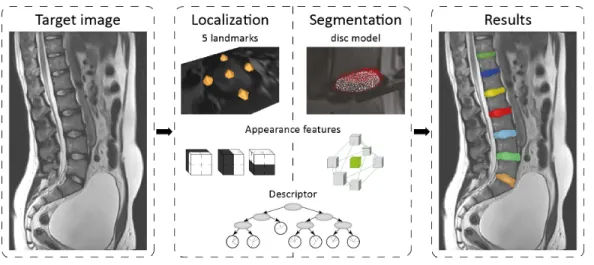
Figure 2: A schematic illustration of the method developed by Korez et al. (Korez et al., 2015a).
3.6. Method of team UNIGRA
The algorithm developed by Urschler et al. (2015) is built upon a machine learning based landmark localization step using regression forests (Gall et al., 2011; Donner et al., 2013) together with a high-level MRF model of the global configuration of the relative landmark positions. While the regression forests predict a number of candidates for each landmark (both IVDs and vertebral bodies) individually, the purpose of the MRF is to select the most probable configuration given the individual voted for locations and the distribution of landmarks in a training data set. After landmark prediction, they develop a three-step image processing pipeline for segmentation. First, they roughly segment vertebral bodies based solely on image gradient information, followed by a merging of pairs of adjacent vertebral bodies to single objects to initialize IVD segmentation. Finally, they formulate the IVD segmentation problem as a convex geodesic active contour (GAC) optimization task based on edges resembling geometrical similarity to the shape of IVDs (Hammernik et al., 2015). Solving the convex GAC model is enabled by a formulation based on weighted total variation and a primal-dual optimization scheme. Enabled by the robustness of previous localization, this latter segmentation step requires no a priori information on appearance but only a very rough shape prior. For more details, we refer to (Urschler et al., 2015).
3.7. Method of team UNILJU
Korez et al. (2015a) propose a supervised framework as shown in Fig. 2 for fully automated localization and segmentation of IVDs from magnetic resonance (MR) images by integrating modern image analysis approaches such as RF-based anatomical landmark detection and surface enhancement, computationally efficient Haar-like features and self-similarity context (SSC) descriptor, and robust shape constrained deformable models.
In their method, IVD localization is performed by detecting its visually distinguishable or anatomically relevant points, i.e. landmarks. Each IVD is described by five landmarks that define its mid-point and most superior, inferior, anterior and posterior points. The properties of these landmarks are studied using training images of manually segmented discs and then used for identification of the same landmarks on a new target image. The intensity appearance of each landmark is captured by Haar-like features, which proved effective for detecting landmarks from MR images of soft tissue (Ibragimov et al., 2015). To minimize landmark mis-detection, for example, when a land-mark is positioned on a neighboring disc, they model the shape of the disc by measuring the pairwise spatial relationships among the landmarks. Optimal landmark positioning is therefore obtained at the point of best agreement between the appearance and shape models (Ibragimov et al., 2014).
IVD segmentation is performed by iterative deformation of the corre-sponding mean disc model towards the edges of the image. As IVD edges are poorly visible on MR images, they propose a RF-based descriptor for disc edge identification. Using training images and corresponding manual segmen-tations, they model the appearance of each edge point as a 26-dimensional feature vector that includes image intensity, Canny edge operator response, gradient orientation and magnitude, SSC features (Heinrich et al., 2013) and other relevant features (Korez et al., 2015b,a). During the segmentation pro-cess, the disc model deforms under the influence of the external energy that moves the model surface towards the detected edge points, and the internal energy that preserves the integrity of the model, its resemblance to the IVD and does not allow its parts to be separated from each other. The final seg-mentation is obtained at the point of equilibrium between the external and internal energy.
3.8. Method of team UNIQUE
The method developed by Neubert et al. (2015) extends and fully auto-mates their previous work on active shape model (ASM) based volumetric
segmentation of lumbar and thoracic IVDs from magnetic resonance (MR) images of the spine (Neubert et al., 2012). The initial version of this algo-rithm was developed for high-resolution volumetric MR images acquired in the axial plane. However, routine clinical examinations are typically acquired using 2D TSE images in the sagittal plane. The original ASM approach was successfully applied to the segmentation of lumbar IVDs from TSE scans by developing a novel initialization scheme. Specifically, an automated localiza-tion approach using multi-atlas registralocaliza-tion and probabilistic shape regres-sion was used to initialize volumetric ASM segmentation driven by grey-level intensity models, as presented in their previous work (Neubert et al., 2012). For details, we refer to (Neubert et al., 2015).
3.9. Method of team VRVIS
Wimmer and Novikov propose a machine learning based pipeline for au-tomated IVD labeling and segmentation. Their method localizes disc center candidates by RF regression (Breiman, 2001) from 2000 sampled positions. They extract 3D Haar-like features (Viola and Jones, 2001) and HOG fea-tures (Dalal and Triggs, 2005) around each position. The HOG parameters were set to 9 orientation bins and a cell size of 8mm. Patch sizes were chosen empirically based on the morphometry of the discs. They propose to extract HOG features from the sagittal and coronal plane to increase the regression efficiency. As a second step, filtering of positions inside discs is performed by SVM classification based on HOG features, whereby 20 best candidates are selected for every disc and the sacrum. Final disc centers are retrieved by ap-plying a graphical model on the filtered disc candidates, similarly to Schmidt et al. (2007). Two connected models are used to reduce the Computational Complexity (CC) of the labeling problem. The first model covers the discs from the sacrum up toL2/L3 and the second model comprises of discsL2/L3 to T11/T12. Due to a higher matching performance of the first model, they made the second model dependent on the matching result of the first one. Finally, IVDs are segmented around the detected centers by a learning-based active contour model built upon a Morphological Active Contour Without Edges (Marquez-Neila et al., 2014). The model is enhanced with RF classi-fiers trained on field-specific, contextual features for each disc separately.
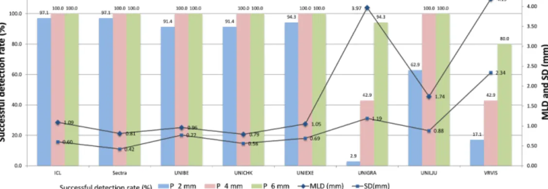
Figure 3: Quantitative evaluation of the localization results for 8 submitted methods on Test1 data.
4. Experimental Results
Quantitative evaluation of the methods of all participating teams is sum-marized in this section. All the methods were evaluated against the ground truth on 10 3D testing volumes, including 5 Test1 volumes and 5 Test2 volumes. In the localization step, 8 teams submitted their automatic IVD localization results except team UNIQUE where they used manual clicks for initialization purpose. Thus we do not include their results for evaluation and comparison. In the segmentation step, all the 9 teams submitted their re-sults obtained on both Test1 data and Test2 data. However, in stage 2, team UNIGRA failed to segment disc T12-T11 in case 5 although they achieved quite good segmentation results in other 4 cases. Thus, we do not include their results for quantitative evaluation and comparison purpose on Test2 data. For all the statistical tests, the significance level is chosen to be 0.01.
4.1. Stage 1
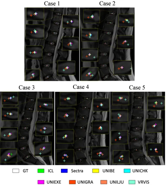
Fig. 3 compares the overall localization results among 8 participating teams in detection of in total 35 IVDs of Test1 data. MLD, SD and SDRs using 3 precision ranges t = 2.0mm, 4.0mm, and 6.0mm (Bars) achieved by these 8 teams are shown in this figure. In Fig.4, we visually compare the ground truth localization with the localization results achieved by all 8 submitted methods on the middle sagittal images extracted from 5 3D MR images of Test1 data.
Figure 4: Visual comparison of localization results for the ground truth (GT) as well as for the 8 submitted methods on Test1 data, where localization results of 7 IVDs on the mid-sagittal slice are shown. The GT localization and the results from different teams are displayed in different color.
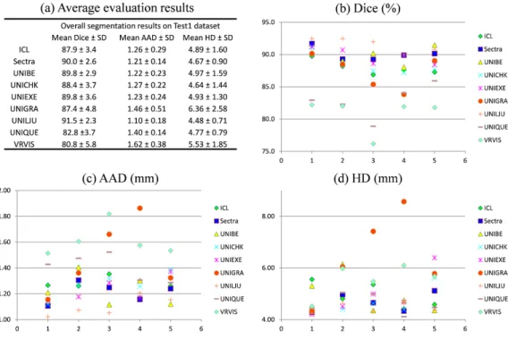
Figure 5: Segmentation results on Test1 data.
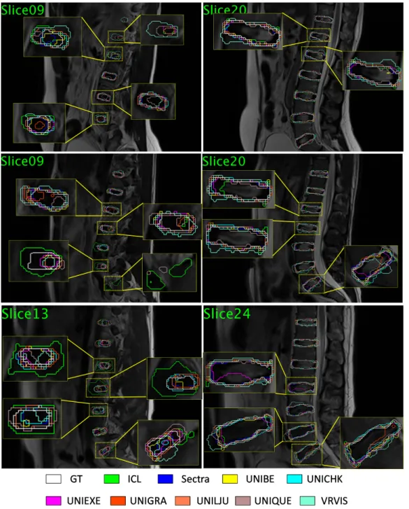
Fig. 5 shows the segmentation results achieved by the 9 participating teams on Test1 data. It compares the overall results of Dice, AAD and HD in segmentation of 35 IVDs between the 9 participating teams on Test1 data. Fig. 5 (b, c, d) present the per case per algorithm evaluation results on Test1 data when we use respectively Dice, AAD, and HD as metrics. Fig. 6 shows the visual comparisons of the segmentation results obtained by all 9 submitted algorithms on 3 cases of Test1 data.
4.2. On-site competition
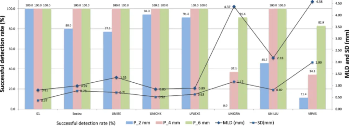
Fig.7 compares the localization results between 8 participating teams in detection of 35 IVDs on Test2 data, which was released for on-site compe-tition. MLD, SD and SDRs using 3 precision ranges t = 2.0mm, 4.0mm, and 6.0mm (Bars) are shown in this figure. Please note that during on-site competition we only allowed maximally one and half hours for each team to finish localization and segmentation of 5 3D T2 MR images. In Fig. 8, we
visually compare the localization results obtained by all teams on each image of Test2 data.
Fig. 9 shows the segmentation results obtained by the 8 participating teams on Test2 data (excluding team UNIGRA). It compares the overall results of Dice, AAD and HD in segmentation of 35 IVDs between the 8 participating teams. In Fig. 9 (b, c, d), theper case per algorithmevaluation results are given when we use respectively Dice, AAD, and HD as metrics for evaluation. Fig. 10 shows the visual comparisons of the segmentation results obtained by all submitted algorithm on 3 cases of Test2 data.
5. Discussions 5.1. Results of stage 1
The performance of the localization methods of the participating teams on Test1 data ranges from 0.79mm to 4.19mm in MLD and 2.9% to 97.1% in SDR for 2.0mm precision range. It is observed that in overall, the best local-ization result on Test1 data is achieved by the method from team UNICHK with the lowest MLD (0.79mm). On the other hand, the method from team Sectra achieves the highest SDR (97.1% ) when evaluated using 2mm preci-sion range and lowest SD (0.42mm). All the 8 submitted methods are able to achieve a SDR better than 80% when the precision range is 6mm and 6 teams are able to achieve a SDR better than 80% when the precision range is 4mm. However, when the precision range is set to 2mm, only 5 teams obtain the SDR better than 80%.
When the localization results are evaluated by MLD and SD, it is ob-served that the top ranked teams such as UNICHK, Sectra, UNIBE, ICL, and UNIEXE achieve quite accurate results that are close to or less than 1.0mm. Paired student’s t-tests were performed to detect whether the dif-ferences between the localization results of different methods are statistically significant. No statistically significant difference was found among the lo-calization results of the 5 top ranked teams, which was consistent with the results shown in Fig. 3. Among the 8 submitted methods, 6 of them are able to achieve MLD lower than 2mm, which is regarded as accurate enough for clinical use (Belavy et al., 2011).
From Fig. 4, it is observed that all the submitted methods are able to localize 35 IVDs with reasonable accuracy although for some cases the localization results are much diverse. Specifically, the localization results for case 4 are quite accurate for all submitted methods and the localization
Figure 6: Visual comparisons of segmentation results on case 1 (top row), 3 (middle row), and 5 (bottom row) of Test1 data. Segmentation contours on 2 typical sagittal slices are shown at each row. The ground truth (GT) segmentation and the segmentation results from different teams are visualized in different colors.
Figure 7: Quantitative evaluation of localization results for 8 teams on Test2 data.
Table 5: Paired student’s t-tests (p-value) to detect whether there are statistically signif-icant differences between the localization results achieved by 8 teams on Test1 data.
Sectra UNIBE UNIEXE ICL UNILJU UNIGRA VRVIS UNICHK 7.8E-01 2.5E-01 2.2E-02 1.6E-02 2.5E-08 4.6E-17 4.6E-10 Sectra 2.8E-01 3.7E-02 2.7E-02 7.8E-08 4.6E-17 3.3E-10 UNIBE 6.0E-01 4.3E-01 3.5E-04 2.6E-16 5.0E-09 UNIEXE 8.1E-01 7.0E-05 7.4E-13 1.8E-08
ICL 4.1E-04 3.0E-14 1.1E-09
UNILJU 2.1E-10 2.0E-06
UNIGRA 6.5E-01
results for case 1 and case 5 are acceptable. However for case 2 and case 3, localization results from team VRVIS are far from the IVD centers such as for IVDs L5-L4 and L4-L3 in case 2, S1-L5 and L5-L4 in case 3.
The performance of the segmentation methods of the participating teams ranges from 80.8% to 91.5% in mean Dice, 1.10mm to 1.62mm in mean AAD, and 4.48mm to 6.36mm in mean HD. It is observed that the best segmenta-tion results is achieved by team UNILJU with an average Dice of 91.5 ± 2.3 %, an average AAD of 1.10 ± 0.18 mm, and an average HD of 4.48 ± 0.71 mm. In overall, all the 9 teams obtain an average Dice greater than 80% and an average AAD lower than 1.7 mm, which are acceptable for clinical practice (Belavy et al., 2011). From the visual comparison as shown in Fig. 6, it is observed that obvious over-segmentation and under-segmentation ex-ist, indicating that this is still a challenging problem and requires further
Figure 8: Visual comparison of the localization results for the ground truth (GT) as well as for the 8 teams on Test2 data, where localization results of 7 IVDs on the mid-sagittal slice are shown. The GT localization and the results from different teams are displayed in different colors.
Figure 9: Segmentation results on Test2 data.
improvement. Paired student’s t-tests are performed to detect whether the differences of the segmentation results (35 IVDs) between different teams are statistically significant and the test results (p-values) are described in Table 6. When we evaluate the segmentation results using Dice as the evaluation metric, it can be found that the differences between team UNILJU and all other 8 teams are of statistical significance (all p-values are less than 0.01), which is consistent with the results reported in Fig. 5. It is also observed that there is no statistically significant difference between team UNIQUE and VRVIS. However, statistically significant differences are found when we compare these 2 teams with other 7 teams. When we evaluate the segmen-tation results using AAD as the metric, again we find that the differences between team UNILJU and almost all other teams are statistically significant (except for team UNIBE where p-value is slightly greater than 0.01). We also find that there are no statistically significant difference between following 5 teams: ICL, Sectra, UNIBE, UNICHK, and UNIEXE. However, when we compare these 5 teams with other two teams such as UNIQUE and VRVIS,
Figure 10: Visual comparisons of segmentation results on case 1 (top row), 3 (middle row), and 5 (bottom row) of Test2 data. Segmentation contours on 2 typical sagittal slices are shown at each row. The ground truth (GT) segmentation and the segmentation results from different teams are visualized in different colors.
Table 6: Paired student’s t-tests (p-value) to detect whether the differences between seg-mentation results obtained from different methods when evaluated on Test1 data are statistically significant. For two metrics used in our study, we conduct t-tests separately.
Dice (%)
Sectra UNIEXE UNIBE UNICHK ICL UNIGRA UNIQUE VRVIS UNILJU 9.6E-04 5.5E-03 1.4E-03 4.2E-06 7.1E-07 3.7E-07 9.7E-14 1.5E-13 Sectra 6.2E-01 4.8E-01 4.9E-04 3.2E-03 2.8E-04 4.4E-13 3.9E-13 UNIEXE 9.9E-01 4.4E-02 4.9E-03 1.4E-03 1.9E-09 2.1E-11
UNIBE 1.2E-02 1.5E-02 2.0E-03 3.3E-11 5.5E-11
UNICHK 5.4E-01 1.3E-01 7.5E-09 1.5E-10
ICL 4.4E-01 2.0E-06 7.5E-08
UNIGRA 3.2E-05 5.8E-10
UNIQUE 4.1E-02
AAD (mm)
Sectra UNIEXE UNIBE UNICHK ICL UNIGRA UNIQUE VRVIS UNILJU 4.0E-03 7.4E-03 1.7E-02 5.7E-04 7.8E-03 2.5E-05 4.9E-08 4.7E-10 Sectra 5.9E-01 6.3E-01 7.1E-02 3.8E-01 2.8E-03 5.3E-06 5.9E-09 UNIEXE 9.9E-01 4.0E-01 6.1E-01 4.1E-03 1.6E-03 1.4E-08
UNIBE 4.4E-01 6.5E-01 6.5E-03 2.6E-03 3.6E-06
UNICHK 9.1E-01 1.6E-02 5.8E-03 1.8E-06
ICL 3.6E-02 6.0E-03 1.0E-04
UNIGRA 4.5E-01 3.1E-02
UNIQUE 2.3E-04
statistically significant differences are observed (p-values smaller than 0.01).
5.2. Results of on-site competition
The performance of the localization methods of the participating teams on Test2 data ranges from 0.81mm to 4.58mm in MLD and 0.0% to 100.0% in SDR for 2.0mm precision range. It is observed that in overall, team ICL obtains the best localization results with the highest SDR (100.0% ) when evaluated using 2mm precision range and the lowest MLD (0.81mm) and SD (0.37mm). When we focus on SDR, all the 8 teams are able to achieve a SDR better than 80% when the precision range is 6mm and 6 teams are able to achieve a SDR better than 80% when the precision range is 4mm. However, when we use 2mm precision range, only 4 teams obtain the SDR better than 80%.
When the localization results are evaluated with MLD, the top ranked 4 teams of ICL, Sectra, UNICHK, and UNIEXE are able to achieve MLD lower than 1.0mm, which is regarded as accurate enough for clinical usage. Paired student’s t-tests are performed to detect whether the differences be-tween different teams in localization of 35 IVDs on Test2 data are statistically
significant and the results are presented in Table 7. No statistically signifi-cant difference is detected among following 4 teams: ICL, Sectra, UNICHK and UNIEXE. These four teams obtain quite accurate localization results as shown in Fig. 7.
From Fig. 8, it is observed that quite promising results are obtained on case 1, case 2, and case 5, even though the appearance around each IVD region is quite different from each other. However, there exist obvious outliers in localization of IVD L3-L2, L2-L1 in case 3 and T12-T11 in case 4 as the results obtained by some teams are out of the IVD regions. These results indicate the room for improvement and need further investigation.
The performance of the segmentation methods of the participating teams on Test2 data ranges from 81.6% to 92.0% in mean Dice, 1.07mm to 1.53mm in mean AAD, and 4.27mm to 5.06mm in mean HD. It is observed that the best segmentation result on Test2 data is achieved by team UNILJU with an average Dice of 92.0 ± 1.9 %, an average AAD of 1.07 ± 0.07mm, and an average HD of 4.33 ± 0.61mm. In overall, all the 8 teams obtain an average Dice greater than 80% and an average AAD lower than 2.0 mm. From the visual comparison as shown in Fig. 10, it is observed that obvious leakage exists, especially in case 3 and case 5 where IVD L1-T12 are severely over-segmented by several teams. Besides over-segmentation, there also exists under-segmentation such as IVD L5-L4 in case 3 and case 4. The experimen-tal results show that it is still an unsolved and challenging task to reduce both over-segmentation (leakage) and under-segmentation and needs further investigation. Paired student’s t-tests are performed to detect whether the differences of the segmentation results (35 IVDs) obtained by different teams are statistically significant and the results are described in Table 8. When we evaluate the segmentation results using both Dice and AAD metric, it is observed that the differences between team VRVIS and the other 7 teams are of statistical significance. We also find that there are no statistically signif-icant differences between following 5 teams such as ICL, Sectra, UNICHK, UNIEXE, and UNIQUE.
5.3. Combined results on Test1 and Test2 data
When we combine results on Test1 and Test2 data (see Table 9 for details), the performance of the localization methods of the participating teams ranges from 0.82mm to 4.39mm in MLD and 1.45% to 98.55% in SDR for 2.0mm precision range. It is observed that in overall, team UNICHK achieves the
Table 7: Paired student’s t-tests (p-value) to detect whether the differences of the local-ization results between different teams on Test2 data are statistically significant.
UNICHK UNIEXE Sectra UNIBE UNILJU UNIGRA VRVIS ICL 6.6E-01 4.2E-01 1.9E-01 9.9E-05 3.7E-11 8.5E-18 5.5E-13 UNICHK 7.7E-01 4.1E-01 6.8E-04 1.2E-09 8.0E-18 1.6E-12 UNIEXE 5.5E-01 2.3E-04 3.9E-08 2.5E-18 1.1E-13 Sectra 3.6E-02 8.9E-07 1.3E-15 7.4E-13 UNIBE 2.7E-04 1.2E-15 1.2E-11
UNILJU 1.1E-10 6.1E-08
UNIGRA 5.9E-01
lowest MLD (0.82mm) and SD (0.49mm) and team ICL achieves the highest SDR (98.55% ) when evaluated using 2mm precision range.
The performance of the segmentation methods of the participating teams on Test1 and Test2 combined data ranges from 81.2% to 91.8% in mean Dice, 1.08mm to 1.57mm in mean AAD, and 4.34mm to 5.09mm in mean HD. It is observed that in overall, team UNILJU achieves the best segmentation results with a mean Dice of 91.8%, a mean AAD of 1.08mm and a mean HD of 4.34mm.
We also compared the results achieved by all teams on Test1 data with those on Test2 data. The average MLD achieved by the localization meth-ods of all teams on Test1 data is 1.83mm while the average MLD on Test2 data is 2.0mm. With 2mm precision range, the average SDR by the local-ization methods of all teams on Test1 data is 69.28% while the average SDR on Test2 data is 62.49%. Such an observation indicates that overall the lo-calization methods of all participating teams perform better on Test1 data than on Test2 data. In contrast, the mean Dice and the mean AAD achieved by the segmentation methods of all teams on Test1 data are 87.6% and 1.29mm, respectively, while the mean Dice and the mean AAD achieved by the segmentation methods of all teams on Test2 data are 89.0% and 1.22mm, respectively. Paired student’s t-tests indicate that there are statistically sig-nificant differences between the segmentation results achieved on Test1 data and those on Test2 data (p-values are smaller than 0.01 for both Dice and AAD metrics). The comparison result indicates that overall the segmenta-tion methods of all participating teams perform worse on Test1 data than on Test2 data. This probably can be explained by our challenge design. Specif-ically, we have 25 3D T2 MR data from two different studies. Our training data in stage 1 contains 10 3D T2 MR data from the first study and 5 3D T2
Table 8: Paired student’s t-tests (p-value) to detect whether the differences of the seg-mentation results between different teams on Test2 data are statistically significant. For two metrics used in our study, we conduct t-tests separately.
Dice (%)
UNIBE UNIEXE Sectra ICL UNICHK UNIQUE VRVIS UNILJU 5.3E-02 8.4E-05 1.2E-06 1.7E-08 9.9E-08 1.5E-09 6.1E-13 UNIBE 1.9E-02 7.0E-03 1.2E-03 1.3E-04 2.4E-06 6.7E-12 UNIEXE 6.0E-01 1.1E-01 5.6E-03 1.1E-03 1.1E-11 Sectra 1.2E-01 5.0E-02 4.6E-03 2.6E-10
ICL 5.7E-01 1.7E-01 3.3E-08
UNICHK 3.9E-01 9.3E-10
UNIQUE 3.6E-09
AAD (mm)
UNIBE UNIEXE Sectra ICL UNICHK UNIQUE VRVIS UNILJU 8.2E-01 7.0E-05 8.3E-07 3.6E-04 4.4E-06 6.1E-12 5.6E-15 UNIBE 3.7E-04 7.4E-06 1.6E-03 3.0E-05 3.1E-09 5.2E-13 UNIEXE 2.0E-01 5.0E-01 5.5E-01 2.8E-01 6.4E-10 Sectra 5.1E-02 4.5E-01 5.8E-01 1.9E-06
ICL 2.4E-01 2.9E-02 2.4E-09
UNICHK 6.0E-01 2.6E-09
UNIQUE 5.0E-08
MR data from the second study while Test1 data is designed to have 4 3D T2 MR data from the first study and 1 3D T2 MR data from the second study and Test2 data is designed to have 1 3D T2 MR data from the first study and 4 3D T2 MR data from the second study. The comparison results indicate that the performance of the localization methods of all participating teams depends more on training data than that of the segmentation methods.
5.4. Computer Specification and efficiency
Details about the computer specification and the efficiency of the 9 par-ticipating teams are presented below. A summary of the details is presented in Table 10.
1. ICL: The pipeline from team ICL has been implemented in Python with some accelerated functions, such as the feature extraction, making use of C++. The authors use the RF and DBSCAN implementations provided in scikit-learn. All the tests were executed on a desktop PC equipped with an Intel Xeon Quad-Core 3.5GHz CPU. Average running
times for the full pipeline including localization and segmentation are about 3 minutes.
2. Sectra: The implementation of the whole segmentation pipeline from team Sectra was primarily done in MATLAB but with the registration implemented in CUDA. The Parallel Computing Toolbox of MATLAB was used to take some advantage of the multi-core architecture of the CPU. The pipeline was executed on a workstation with Windows 7 SP1 (x64), MATLAB 2014b and CUDA 5.5. The CPU was an Intel Core i7 960 with four cores with 24 GB of RAM and the GPU was a GeForce GTX 660 Ti with 1344 CUDA cores. The complete processing time for a single data set was approximately 8 minutes and 30 seconds with 1 minute and 15 seconds for detection and labeling, 7 minutes and 10 seconds for registration and 5 seconds for label fusion.
3. UNIBE: The algorithm was implemented in Matlab for Data-driven based method and in C++ for multi-atlas fusion based graph cut method. The unoptimized implementation requires on average 18 min-utes to localize and segment one subject on a laptop with 3.0 GHz CPU and 12 GB RAM, where it takes about 3 minutes to do a rough localization and segmentation and the rest 15 minutes to finish the multi-atlas-based segmentation.
4. UNICHK: DeepSeg-3D was implemented with Python3 based on the Theano library and it took about 0.3 seconds to process one test image with size 40×512×512 using a standard PC with a 2.50 GHz Intel(R) Xeon(R) E5-1620 CPU and a NVIDIA GeForce GTX X GPU., which was much faster with one single forward propagation.
5. UNIEXE: The implementation was written in MATLAB with C++ code for computationally intensive tasks including supervoxel genera-tion, SVM optimisation and computation of the CRF max-marginals. The execution time for processing a single volume after learning was approximately 6 min using an Intel Core i5 2.50 GHz machine with 8GB of RAM running Linux (64-bit).
6. UNIGRA: The whole localization and segmentation approach was implemented in C++ and OpenMP, with the exception of the Matlab-based MRF solver. Costly image processing operations were accelerated using NVidia’s CUDA environment. The algorithm was executed on a notebook with an Intel Core i7-4700HQ CPU, 16 GByte of RAM, an NVidia Geforce GTX 760M GPU with 2GB of RAM, running Ubuntu Linux 15.04. The running time for localization and segmentation was
around 8 minutes per data set, where the computational effort goes roughly half into localization and segmentation, respectively.
7. UNILJU: The detection and segmentation parts of the framework were implemented using C++ and Matlab. The experiments were exe-cuted on a personal computer with Intel Core i5 processor at 3.20 GHz and 16GB of memory without a graphical processing unit. The detec-tion of all seven IVDs took on average 85s, whereas the segmentadetec-tion of each individual IVD took on average 30s.
8. UNIQUE: The methods were implemented in C++ using Insight Seg-mentation and Registration Toolkit (ITK) and Visualization Toolkit (VTK) libraries for image and mesh processing, an in-house C++ soft-ware library for statistical shape modeling and visualization. The ex-periments were run on a desktop computer Intel(R) Core(TM) i7-4770 CPU @ 3.40GHz with 32 GB RAM memory under Ubuntu 14.04 LTS. Using 8 threads, on average it took about 4 minutes to segment one data set with 7 IVDs.
9. VRVIS: The complete framework was implemented in Java. All test-ing experiments were conducted on an Intel Xeon E5-2620 v3 windows machine with 16 GB of RAM. Overall processing time for disc local-ization and segmentation of one data set is around 4.2 minutes. The bottleneck in terms of computation time is the disc and sacrum classifi-cation with SVMs. Even though they use multi-threading in this stage, this step is the most expensive part with a runtime of approx. 2.7 min-utes. The rest of the pipeline runs in a single-threaded environment. Feature calculation and regression take around 30 seconds, the appli-cation of the graphical model around 50 seconds and the segmentation of all discs only around 10 seconds.
5.5. Analysis of advantages and drawbacks of all methods
The advantages and drawbacks of all methods are summarized in Fig. 11. From the results presented in Sections from 5.1 to 5.3, the method of team UNICHK shows the best localization performance in this challenge while the method of team UNILJU shows the best segmentation performance.
For localization, the crucial difference that makes the method of team UNICHK superior to other competitors is the deep segmentation network which leverages flexible 3D convolution kernels by considering spatial infor-mation for a fast speed with volume-to-volume classification. Their method
Table 9: Combined Results on Test1 and Test2 Data
Overall Localization Results (Measured with MLD)
Rank Team Name Test1 Results (mm) On-site (Test2) Results (mm) Average (mm)
1 UNICHK 0.79±0.56 0.85±0.52 0.82±0.54 2 Sectra 0.81±0.42 0.99±0.78 0.90±0.60 3 ICL 1.09±0.60 0.81±0.37 0.95±0.49 4 UNIEXE 1.05±0.69 0.89±0.63 0.97±0.66 5 UNIBE 0.96±0.77 1.35±0.71 1.16±0.74 6 UNILJU 1.74±0.88 2.18±0.82 1.96±0.85 7 UNIGRA 3.97±1.19 4.37±1.17 4.17±1.18 8 VRVIS 4.19±2.34 4.58±1.99 4.39±2.17
Overall Segmentation Results (Measured with Dice Overlap Coefficients) Rank Team Name Test1 Results (%) On-site (Test2) Results (%) Average (%)
1 UNILJU 91.5±2.3 92.0±1.9 91.8±1.2 2 UNIBE 89.8±2.9 91.2±2.0 90.5±1.4 3 UNIEXE 89.8±3.6 90.2±2.6 90.0±1.7 4 Sectra 90.0±2.6 90.0±2.2 90.0±1.3 5 UNICHK 88.4±3.7 88.9±3.4 88.6±1.8 6 ICL 87.9±3.4 89.3±2.6 88.6±1.2 7 UNIQUE 82.8±3.7 88.4±2.9 85.6±3.5 8 VRVIS 80.8±5.8 81.6±6.4 81.2±3.6
Table 10: Details on computation time and computer systems used for the different al-gorithms. We indicate whether an algorithm uses multi-threaded (MT) or graphical pro-cessing unit (GPU).
Team name
Avg.
time System MT GPU
Programming Language Remarks ICL 3 min 3.5 GHz 4-cores No No Python and C++ RF and DBSCAN implemented in scikit-learn Sectra 8.5 min 3.2 GHz
4-cores Yes Yes
Matlab and Cuda GeForce GTX 660 Ti with 1344 CUDA cores UNIBE 18 min 3.0 GHz 4-cores No No Matlab and C++ UNICHK 0.3 s 2.5 GHz
4-cores Yes Yes Python UNIEXE 6 min 2.5 GHz
4-cores Yes No
Matlab and C++ UNIGRA 8 min 2.4 GHz
4-cores Yes Yes
C++ and Matlab UNILJU 5 min 3.2 GHz 4-cores No No C++ and Matlab UNIQUE 4 min 3.4 GHz 4-cores Yes No C++
Requires manual localization of the first IVD
VRVIS 4.2 min 2.4 GHz
6-cores Partially No Java
Mixture of multi-threaded with single-threaded
Table 11: Comparison of two different methods from team UNICHK for IVD localization. Method MLD(mm) SD(mm) SDR with t = 2.0mm SDR with t = 4.0mm SDR with t = 6.0mm DeepSeg-2D 1.07 0.62 91.4% 100% 100% DeepSeg-3D 0.91 0.58 94.3% 100% 100% Combined Results 0.79 0.56 91.4% 100% 100%
takes a volume as input and generates a volumetric segmentation mask within one single forward propagation without restoring to a sliding window strat-egy. Thus, their localization method is not only the most accurate one but also the fastest one. To confirm this assumption, Chen et al. (2015b) imple-mented another type of deep neural networks by making use of adjacent slices (the kernal size of the third dimension is 3) and refer this one asDeepSeg-2D. The performance of DeepSeg-2D was compared with that of DeepSeg-3D on Test1 data and the results are presented in Table 11.
For segmentation, the crucial difference that makes the method of team UNILJU superior to other competitors is the efficient combination of machine learning and shape constrained deformable models. This has been observed in several other top ranked segmentation methods, i.e., efficient integration of learned likelihood terms within different types of energy minimization-based segmentation framework.
6. Conclusion
The paper presents the construction of a manually annotated reference data set composed of 25 3D T2-weighted TSE MR images acquired from two different studies and the establishment of a standard framework for an objec-tive comparison of a representaobjec-tive selection of the state-of-the-art methods that were submitted to the Automatic MRI IVD Localization and Segmen-tation Challenge held at MICCAI 2015. A total of ten teams submitted their results in Test1 data, and all of them were accepted to the on-site competi-tion. Results from 9 teams were included in this study.
It is worth to point out the limitations of the challenge. Although the 25 3D T2-weighted MR data set used in this challenge are from two different studies investigating the IVD morphology change after prolonged bed test, all the participants included in these two studies are medically and
psychologi-cally healthy subjects. Though the majority of the methods of participating teams achieved quite accurate results, further investigation is required to see whether similar results can be obtained when evaluated on data acquired from patients with severe pathology.
The evaluation of changes in IVDs with MR images can be of interest for many applications beyond IVD degeneration quantification. For example, it is important to know the changes of IVDs during prolonged bed rest which is used to understand the effects of inactivity on the human body and to simulate the effects of microgravity on human body by space agencies (Belavy et al., 2012, 2011). At this moment, clinicians lack tools to conduct a true 3D quantification even when 3D MR image data are available. Instead, they seek to use 2D surrogate measurements measured from selected 2D slices to quantify 3D spinal morphology (Belavy et al., 2012, 2011). Automated methods save time and manual cost, and allow for a true 3D quantification avoiding problems caused by 2D measurements.
7. Acknowledgements
The paper is partially supported by the Swiss National Science Foun-dation Project No. 205321−157207/1. The acquisition of original images was supported by the Grant 14431/02/N L/SH2 from the European Space Agency, grant 50WB0720 from the German Aerospace Center (DLR) and the Charit´e University Medical School Berlin. The work of team UNILJU was partially supported by the Slovenian Research Agency, under grants P2−0232, J2−5473, J7−6781 and J7−7118. The work of team ICL was partially funded by the Dunhill Medical Trust, R401/0215. I. L´opez An-drade is supported by the Fundaci´on Barri´e. D. Forsberg was funded by the Swedish Innovation Agency (VINNOVA, grant 2014-01422). H. Chen and D. Qi were funded by Hong Kong RGC Fund (Project No. CUHK 412513). M. Urschler was partially funded by province of Styria, ABT08-22-T-7/2013-13, and D. Stern by Austrian Science Fund (FWF), P28078-N33. The work of team UNIQUE was partially supported under Australian Research Coun-cil’s linkage project funding scheme LP100200422. The competence center VRVis with the grant number 843272 is funded within the scope of COMET. Achanta, R., Shaji, A., Smith, K., Lucchi, A., Fua, P., Susstrunk, S., 2012. Slic superpixels compared to state-of-the-art superpixel methods. IEEE Trans. Pattern Anal. Mach. Intell. 34 (11), 2274–2282.
Ali, A., Aslan, M., Farag, A., 2014. Vertebral body segmentation with prior shape constraints for accurate BMD measurements. Comput Med Imaging Graph 38 (7), 586595.
Alomari, R., Corso, J., Chaudhary, V., 2011. Labeling of lumbar discs using both pixel- and object-level features with a two-level probabilistic model. IEEE Trans Med Imaging 30 (1), 1–10.
Andersson, G., 2011. The burden of musculoskeletal diseases in the United States: prevalence, societal and economic cost. American Academy of Or-thopaedic Surgeons, Ch. 2, ”Spine: Low back and neck pain”,, pp. 21–56. Belavy, D., Armbrecht, G., Felsenberg, D., 2012. Incomplete recovery of lum-bar intervertebral discs 2 years afer 60-days bed rest. Spine 37 (14), 1245– 1251.
Belavy, D., Bansmann, P., Boehme, G., Frings-Meuthen, P., Heer, M., Rit-tweger, J., Zhang, J., Felsenberg, D., 2011. Changes in intervertebral disc morphology persist 5 mo after 21-day bed rest. J App Physiol 111, 1304– 1314.
Ben Ayed, I., Punithakumar, K., Garvin, G., Romano, W., Li, S., 2011. Graph cuts with invariant object-interaction priors: application to inter-vertebral disc segmentation. In: Proceedings of IPMI2011. pp. 221–232. Boykov, Y., Funka-Lea, G., 2006. Graph cuts and efficient n-d image
seg-mentation. Int. J. Comput. Vis. 70 (2), 109–131.
Breiman, L., 2001. Random forests. Machine learning 1, 5–32.
Cai, Y., Osman, S., Sharma, M., Landis, M., Li, S., 2015. Multi-modality vertebra recognition in artbitray view using 3d deformable hierarchical model. IEEE Trans Med Imaging 34 (8), 1676–1693.
Carballido-Gamio, J., Belongie, S., Majumdar, S., 2004. Normalized cuts in 3-d for spinal mri segmentation. IEEE Trans Med Imaging 23 (1), 36–44. Chen, C., Belavy, D., Yu, W., Chu, C., Armbrecht, G., Bansmann, M.,
Felsenberg, D., Zheng, G., 2015a. Localization and segmentation of 3d intervertebral discs in mr images by data driven estimation. IEEE Trans Med Imaging 34 (8), 1719–1729.
Chen, H., Dou, Q., Wang, X., Heng, P.-A., 2015b. Deepseg: Deep segmen-tation network for intervertebral disc localization and segmensegmen-tation. In: Proc. 3rd MICCAI Workshop & Challenge on Computational Methods and Clinical Applications for Spine Imaging - MICCAI-CSI2015.
Chen, H., Shen, C., Qin, J., et al., 2015c. Automatic localization and identi-fication of vertebrae in spine ct via a joint learning model with deep neural network. In: Proceedigns of MICCAI 2015. Vol. Part I, LNCS 9349. pp. 515–522.
Cheung, K., Karppinen, J., et al., 2009. Prevalence and pattern of lumbar magnetic resonance imaging changes in a population study of one thousand forty-three individuals. Spine 34 (9), 934–940.
Chevrefils, C., Cheriet, F., Aubin, C., G, G., 2009. Texture analysis for automatic segmentation of intervertebral disks of scoliotic spines from mr images. IEEE Trans Inf Technol Biomed. 13 (4), 608–620.
Chevrefils, C., ChEriet, F., Grimard, G., Aubin, C., 2007. Watershed seg-mentation of intervertebral disk and spinal canal from mri images. In: Proceedings of ICIAR 2007, LNCS 4633. pp. 1017–1027.
Chu, C., Yu, W., Li, S., Zheng, G., 2015. Localization and segmentation of 3dintervertebral discs from mr images via a learning based method: a validation framework. In: Proc. 3rd MICCAI Workshop & Challenge on Computational Methods and Clinical Applications for Spine Imaging -MICCAI-CSI2015. pp. 135–143.
Corso, J., Alomari, R., Chaudhary, V., 2008. Lumbar disc localization and labeling with a probabilistic model on both pixel and object features. In: Proceedings of MICCAI2008. Vol. Part I. pp. 202–210.
Criminisi, A., Robertson, D., Konukoglu, E., et al., 2013. Regression forests for efficient anatomy detection and localization in computed tomography scans. Med Image Anal 17 (8), 1293–1303.
Dalal, N., Triggs, B., 2005. Histograms of oriented gradients for human de-tection. In: Proceedings of CVPR 2005. Vol. 1. pp. 886–893.
Dice, L., 1945. Measures of the amount of ecologic association between species. Ecology 26 (3), 297–302.