Air Force Institute of Technology
AFIT Scholar
Theses and Dissertations Student Graduate Works
3-23-2018
Target Detection using Convolutional Neural
Networks
Robert P. Loibl
Follow this and additional works at:https://scholar.afit.edu/etd
Part of theArtificial Intelligence and Robotics Commons, and theTheory and Algorithms Commons
This Thesis is brought to you for free and open access by the Student Graduate Works at AFIT Scholar. It has been accepted for inclusion in Theses and Dissertations by an authorized administrator of AFIT Scholar. For more information, please [email protected].
Recommended Citation
Loibl, Robert P., "Target Detection using Convolutional Neural Networks" (2018).Theses and Dissertations. 1814. https://scholar.afit.edu/etd/1814
TARGET DETECTION USING CONVOLUTIONAL NEURAL NETWORKS THESIS
Robert P. Loibl, Captain, USAF AFIT-ENG-MS-18-M-043
DEPARTMENT OF THE AIR FORCE AIR UNIVERSITY
AIR FORCE INSTITUTE OF TECHNOLOGY
Wright-Patterson Air Force Base, Ohio DISTRIBUTION STATEMENT A.
The views expressed in this thesis are those of the author and do not reflect the official policy or position of the United States Air Force, Department of Defense, or the United States Government. This material is declared a work of the U.S. Government and is not subject to copyright protection in the United States.
AFIT-ENG-MS-18-M-043
TARGET DETECTION USING CONVOLUTIONAL NEURAL NETWORKS THESIS
Presented to the Faculty
Department of Electrical and Computer Engineering Graduate School of Engineering and Management
Air Force Institute of Technology Air University
Air Education and Training Command In Partial Fulfillment of the Requirements for the Degree of Master of Science in Computer Engineering
Robert P. Loibl, BS Captain, USAF
March 2018
DISTRIBUTION STATEMENT A.
AFIT-ENG-MS-18-M-043
TARGET DETECTION USING CONVOLUTIONAL NEURAL NETWORKS
Robert P. Loibl, BS Captain, USAF Committee Membership: Dr. Kenneth M. Hopkinson Chair Dr. Bryan J. Steward Member Dr. Kevin C. Gross Member
AFIT-ENG-MS-18-M-043
Abstract
This research explores the use of Convolutional Neural Networks (CNNs) to classify targets of interest within satellite imagery. Methods were specifically devised for the classification of airports within Landsat-8 scenes. A novel automated dataset
generation technique was developed to create labeled datasets from satellite imagery using only coordinate metadata. Using this approach a very large dataset of over 132,000 labeled images was created without human input. This dataset was used to evaluate the effects of color and resolution on airport classification accuracy. Two experiments were run with the first experiment classifying large airports with 96.8% accuracy, and the second classifying large and medium airports with 90.2% accuracy. Additionally, a new algorithm was developed which optimizes the selection of multi-spectral color bands in order to best trade-off classification accuracy for the number of spectral bands employed.
Acknowledgments
I would like to express my sincere appreciation to my faculty advisor, Dr. Kenneth M. Hopkinson, for his guidance and support throughout the course of this thesis effort. Additionally I would like to thank my sponsor, the AFRL Space Vehicles Directorate for both their support and interest in this research.
Table of Contents
Page
Abstract ... iv
Table of Contents ... vi
List of Figures ... viii
List of Tables ...x
I. Introduction ...1
Topic & Motivation ...1
Structure of This Paper ...5
Research Goals & Application ...5
Notional Problem...6
II. Background ...11
Perceptron ...11
Multilayer Perceptrons ...13
Convolutional Neural Networks ...14
Supervised Learning ...15
Regularization ...16
Activation Functions ...17
III. Methodology ...18
Datasets...18
First Experiment Methodology...30
Second Experiment Methodology ...37
IV. Analysis and Results ...42
Experiment One ...42
V. Conclusion ...53 Future Work...53 Recommendations ...55 Appendix ...56 dataset_gen_master.py ...56 fix_airport_names.py ...58 Autotiling_Multicore.py ...61 Autotiling_Functions.py ...63 autotiling_check.py ...68 darkness_filter.py ...69 consolidate_bands.py...71 gen_npy_images.py ...74 dictionary_gen.py ...77 Bibliography ...78
List of Figures
Page
Figure 1. Lansat-8 Tiles ...7
Figure 2. DigitalGlobe Image ...9
Figure 3. Perceptron ...12
Figure 4. Artificial Neural Network ...13
Figure 5. Convolution Operation ...14
Figure 6. Activation Functions ...17
Figure 7. Automated Dataset Generation Pipeline ...22
Figure 8. Targets CSV Excerpt ...23
Figure 9. Landsat-8 Invalid Regions of Scene ...23
Figure 10. Imagery Download GUI ...24
Figure 11. All-Tiling Algorithm ...26
Figure 12. Adjacent Tiling Algorithm ...27
Figure 13. Tiling Speedup with Multi-Processing ...28
Figure 14. Auto-Tiling Example ...30
Figure 15. Custom VGG-19 Architecture ...35
Figure 16. Grayscale 3-Color Diagram ...36
Figure 17. SqueezeNet Architecture ...39
Figure 18. Fire Module ...40
Figure 19. Test Accuracy ...43
Figure 20. Training & Validation History ...46
Figure 22. Validation Accuracy Selected Models ...48
Figure 23. Probability Distribution Grayscale Models ...51
Figure 24. Probability Distribution Multi-Color Models ...51
List of Tables
Page
Table 1. Selected Landsat-8 Bands ...8
Table 2. Worldview-3 Bands ...9
Table 3. Worldview-4 Bands ...9
Table 4. Hardware Configuration ...28
Table 5. Experiment One Dataset ...31
Table 6. Experiment Two Dataset ...37
Table 7. Experiment One Hyper-Parameters ...43
Table 8. Experiment One Test Accuracy ...44
Table 9. Experiment Two Hyper-Parameters ...45
Table 10. Experiment Two Grayscale Test Accuracy ...49
Table 11. Experiment Two Greedy CA Metric ...49
Table 12. Experiment Two Greedy Correlation Metric ...49
Table 13. T-Test 2-Color Network ...50
TARGET DETECTION USING CONVOLUTIONAL NEURAL NETWORKS I. Introduction
Topic & Motivation
The Air Force is facing a new emerging capability gap brought about by the very data its own systems generate. The Air Force, and by extension the Department of Defense (DoD), operate one of the largest and most robust reconnaissance programs in history, gathering and moving massive amounts of data every day. Today turning data into information is largely a human enterprise where intelligence analysts examine Remote Sensing (RS) imagery and fuse multiple data sources to create new information products. Information is then used in turn as the primary tool for military commanders to make decisions. The DoD recognizes the importance of information in military
operations and actively pursues Information Superiority against its adversaries [1]. As the Air Force continues to deploy new and more capable sensors to maintain its information advantage, the resources needed to make sense of the incoming data increases. Large amounts of collected data is not used and most data is not exploited to its fullest extent due to manpower limitations. This gap between collected data and produced information threatens the DoD’s ability to maintain Information Superiority in the future.
The data to information gap is a serious problem that manifests itself throughout Air Force operations. The speed at which data can be processed and turned into
information affects the pace at which decisions can be made. If more data could be processed at a faster rate new operations would become feasible that currently cannot be undertaken. Unfortunately information creation is dependent on limited human resources,
which are unable to deal with the volume of data and the speed at which information needs to be created for new operations. However another option exists to augment and enhance current data processing methods; Artificial Intelligence (AI). AI is a loose
collection of algorithmic methods that involve learning, emergent behavior, and advanced problem solving. Specifically this research focuses on the disciplines of machine learning and deep learning.
Automation and AI are already being broadly pursued by the Air Force and the DoD as a whole. To highlight the significance of automation to future Air Force
operations “Machine to machine options for turning data into information” is listed as a key capability in the Air Superiority 2030 Flight Plan [2] chartered by the Chief of Staff of the Air Force (CSAF). Human and machine teaming systems also present a near term option to improve the performance of aircraft, Intelligence Surveillance Reconnaissance (ISR), data exploitation, and Communications Command Control (C3). These
technologies have the potential of becoming a potent force multiplier for future
operations, which is why AI is often cited as a critical component of the so called “Third Offset” [3], allowing whomever masters autonomy to overwhelm their adversaries.
One specific area which is ripe for autonomy is the RS field. Modern AI
techniques that have seen success in other commercial domains can be applied to RS data to great effect. Solving the data to information gap for RS imagery using Deep
Convolutional Neural Networks (DCNNs) [4] [5] [6] [7] is the focus of this research. Classifying and localizing objects within images using CNNs is an ongoing area of research [8] [9] [10], and there are specific considerations when applying these techniques to RS data. Several challenges exist that make the RS domain particularly
difficult for machine learning; these include large image size, lack of existing datasets for training, unsupported image formats, proprietary and/or classified data, and small object to image ratios. Despite all of these challenges there are also attributes of this imagery that are beneficial and allow new approaches to be explored.
The first is that almost all satellite imagery contains geographic metadata which can be used in conjunction with object localization to determine a point on earth where the target is located. It can also be used with a known list of object coordinates to create a new labeled dataset. Coordinate information already exists for many objects of interest such as airports, ports, buildings, ships, airplanes, and cars. Cross referencing the locations of these objects within existing satellite scenes of the earth requires a simple search algorithm or database request. Using this method large datasets can be created in an automated fashion. The second benefit is that the coordinates of any detected object can be used as part of a larger system. Automated target detection yielding earth
coordinates can be used in a satellite tipping and cueing system. The scenario is as such; one satellite takes an image of the earth, the image is processed using a neural network which yields a potential detection of a target, another satellite is cued to collect further data at the coordinates of the initial target. A third unique attribute is that in addition to typical RGB images, satellites image the earth in various spectral bands [11]. These bands yield additional characteristic information about a target that can increase
classification accuracy. Networks trained on multi-spectral image data could potentially analyze an image across dozens of bands simultaneously.
Initial research has begun in the last few years to exploit hyperspectral imagery using CNNs and also to apply CNNs, as well as Recurrent Neural Networks (RNNs), to
satellite imagery. One common approach deals with the lack of labeled hyperspectral training data by training an un-supervised network on generic image data and then applying this network to a small amount of curated and labeled hyper-spectral data [12] [13]. Using unsupervised learning a feature extractor can be created that is generalized enough to also extract salient features from hyper-spectral data. Two self-taught frameworks were tested: the multiscale ICA and the stacked convolutional encoder. These frameworks achieved good results against various existing hyperspectral datasets, but no analysis was done to determine the effect of hyper-spectral data on the achieved accuracy or the extracted features. Research on localizing objects and implementing pixel-wise classification has also been undertaken using hyper-spectral imagery. Using a modified VGG-16 network [5] with its fully connected layers replaced by convolutional layers a hyper-spectral feature map can be created and used for pixel-wise classification [14] [13]. This research also notes the primary disadvantage of pre-training from non-hyper-spectral datasets, which is the reduction in the use of non-hyper-spectral only features. The end effect of this is an overall reduction of information presented to the network. Using the modified VGG network impressive segmentation maps of the earth were produced, which classified RS imagery by terrain. In addition to the natural use of CNNs to classify RS imagery, RNNs have also been proposed as a feature extractor in hyper-spectral imagery [15]. RNNs are typically used in scenarios where temporal or sequential information is important for accurate classification. When using an RNN for imagery the color bands themselves are fed into the network sequentially. This framework exploits the naturally sequential nature of hyper-spectral image data and represents a significant
departure from other work in the field. Ultimately it was found that RNNs can outperform CNNs when used on imagery with many spectral bands.
Structure of This Paper
Section I continues by discussing the goals of this research and laying out the notional Landsat-8 airport detection problem. Section II covers in detail some of the key AI technologies utilized in this research. In Section III the research methodology is laid out, starting with the automated dataset generation and then the setup and motivation behind each of the two experiments. Section III also explores some of the options considered for two key decisions: the selection of the imagery dataset, and the network architectures for each experiment. Section IV reports the results from both experiments and provides an analysis on the outcomes. Finally Section V provides the conclusions that can be drawn about multi-spectral image classification based on the experimental testing.
Research Goals & Application
This research aims to explore three goals: demonstrate the application of commercial deep learning methods for military missions, understand the specific considerations that the RS domain requires in creating AI systems, and investigate the benefit of multi-spectral information to object detection & classification.
As mentioned before many area of the military can benefit from the introduction of autonomous systems. Two specific military applications that would benefit greatly from this research are satellite tipping & cueing systems and data pre-processing systems for use by intelligence analysts. A data triage system as imagined in this research is a
system in which all incoming remote sensing imagery is fed through. It is a neural network trained to detect a set of military targets within imagery. Such a system can take a “first look” through all data to find the most likely target locations for further
investigation by human analysts. These types of human & machine systems are necessary to deal with the increasing volume of incoming data. One way in which a data triage system could take shape is as a heat map of detections overlaid on an RS image. Rather than having an operator search “cold” through the entire image, they can start looking immediately at the “hottest” area of the image. If there are multiple target types each heat map could be saved as a separate channel, allowing the operator to switch focus between targets of interest.
Notional Problem
Research will be conducted by exploring a notional problem to develop tools and methods in an unclassified and simple environment. When deciding on an imagery source and notional target the two main methods of collecting RS data were considered; airborne or space borne collection. The decision was made to focus specifically on RS imagery obtained from satellite payloads. However the methods used could also be applied to imagery obtained via aircraft with slight modifications to data collection and training. The choice of satellite imagery over aircraft imagery is due to several factors, the first being there is better global coverage using satellite imagery as opposed to airborne images. The second factor is that many satellite images have a fixed viewpoint caused by the camera being so far away from the target. This causes images to have a “directly” overhead orientation. When training a neural network differences in orientation make
classification much more difficult. Many airborne camera take images from varying heights, as well as off the side of the plane. This causes the resulting images to be taken from many angles. The expectation then is that more images would be needed or more extensive data augmentation in order to train a network to sufficient accuracy. One drawback to the satellite only approach is that the images are often of a lower spatial resolution, which limits the choice of targets available to train on.
Figure 1. Landsat-8 Images of airports courtesy of the U.S. Geological Survey. Images in the upper left are grayscale, and images in the lower right are composite RGB. All
images shown have a spatial resolution of 30m/pixel
Two satellites have been identified as sources of training data for the planned CNNs. The first is the Landsat-8 earth observation satellite [11]. This mission of the Landsat series of satellites is to conduct a long term geological survey of the earth. The satellite carries two sensors, the first is an Operational Land Imager (OLI) and the second is a Thermal Infrared Sensor (TLI). These two sensors together support data acquisition
from 11 different spectral bands. Of the 11 available bands, 7 are of specific interest to my research. These bands are shown in Table 1.
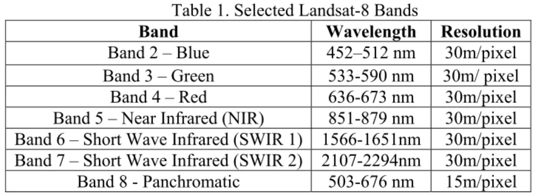
Table 1. Selected Landsat-8 Bands
Band Wavelength Resolution
Band 2 – Blue 452–512 nm 30m/pixel
Band 3 – Green 533-590 nm 30m/ pixel
Band 4 – Red 636-673 nm 30m/pixel
Band 5 – Near Infrared (NIR) 851-879 nm 30m/pixel Band 6 – Short Wave Infrared (SWIR 1) 1566-1651nm 30m/pixel Band 7 – Short Wave Infrared (SWIR 2) 2107-2294nm 30m/pixel
Band 8 - Panchromatic 503-676 nm 15m/pixel
These bands were selected because they provided images of the earth’s surface, rather than aerosols or cloud cover. They also cover the standard RGB colors, as well as additional infrared colors. Finally the panchromatic band allows comparisons between resolution and color to be made. All bands have the same ground resolution of 30 meters per pixel, except for the panchromatic band. This resolution allows for large stationary objects to be used as targets. Some targets that fit this description are cities, military bases, rail stations, ports, and airports. Each Landsat scene covers a broad section of the earth in all bands, the Field of View (FOV) for the payloads is 185 km. The resulting images are about 60mb per image, with the panchromatic images being larger at around 100mb per image. All Landsat data is hosted free of charge on Amazon Web Services (AWS) https://aws.amazon.com/public-datasets/landsat/.
The second source of imagery is from the DigitalGlobe constellation [16] [17]. DigitalGlobe is a commercial company that provides RS imagery at a very high
Worldview-4. Both satellites collect visible and NIR bands at 1.24m/pixel and panchromatic at 31cm/pixel.
Figure 2. DigitalGlobe Image of Airport (1.24m/pixel) Table 2. Worldview-3 Bands
WorldView-3
Band Wavelength Resolution Blue 445-517 nm 1.24m/pixel Green 507-586 nm 1.24m/pixel Red 626-696 nm 1.24m/pixel NIR 765-899 nm 1.24m/pixel Panchromatic 450-800 nm 31cm/pixel
Table 3. Worldview-4 Bands WorldView-4
Band Wavelength Resolution Blue 450-510 nm 1.24m/pixel Green 510-580 nm 1.24m/pixel
Red 655-690 nm 1.24m/pixel
NIR 780-920 nm 1.24m/pixel
The DigitalGlobe constellation offers the best resolution imagery in the commercial market and opens up many more targets for training. In theory any target resolvable at 31cm/pixel could be used for training, however the following targets have been identified: ships, airplanes, mobile launchers, tanks, and artillery. All of these targets are non-stationary targets that generally relocate about the earth. When compared to the stationary targets that could be trained on with Landsat-8, these targets are much more interesting. Of course because these targets are moving all training examples will need to be found by using a location and a time, which increases the difficulty of acquiring a dataset.
Taking into account the two aforementioned data sources and the potential targets for each It was decided that the research would focus on a notional problem in order to develop generalized tools and methods to train CNNs on RS images.
The imagery source chosen for the primary focus was the Landsat-8 satellite. This was for a couple of reasons: the first is that there is overall more images of the earth available from the Landsat database than DigitalGlobe. This allows for more training examples to be generated for the dataset and improves the odds of success during
training. Currently the Landsat-8 database contains over 700,000 scenes of the earth. The second reason is that the size of each Landsat image is much smaller than each
DigitalGlobe image. In fact the average size of a Landsat Image is about one tenth the size of a DigitalGlobe image. Since all images must be downloaded from the web, image size has a huge impact on the amount of training examples that can be obtained for the dataset.
The chosen goal is the detection of large and medium airports. Airports were chosen as the target because of their large size, distinctive characteristics, fixed locations, and known geographic coordinates. It was of particular importance that the selected target have known “truth” coordinates so that an automated dataset generation technique could be used. Other moving targets presented a particular challenge when trying to bring together this “truth” information. In future research it may be worthwhile to investigate the acquisition of coordinate information from cars, ships, and planes. Coordinates and earth locations at a certain time could be determined by using combinations of Automatic Identification System (AIS), transponders, and Global Positioning System (GPS)
information. However such a task is much harder than simply acquiring a coordinate list of airports around the world and would likely distract from the real research objectives.
II. Background Perceptron
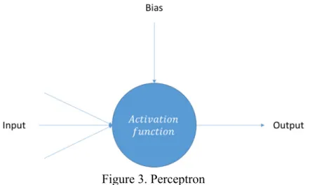
The perceptron is the most basic building block of a neural network. It is often depicted as a single node with several incoming edges and a single outgoing edge. The design of the perceptron was originally inspired by the biological neuron and is also sometimes referred to as an artificial neuron [18]. Figure 3 shows the layout of a single perceptron, with three input edges and one output edge.
Figure 3. Perceptron
The perceptron functions by first multiplying each input by the associated weight of the incoming edge. Then the product is summed for all of the incoming edges, with the bias added, and then this result is modified through the use of an activation function.
∗ ∈
(1)
, ,
Many activation functions exist with the two most popular being the sigmoid and Rectified Linear Unit (ReLU). One major drawback of single perceptrons is that they can only linearly separate classes, and even simple problems such as the XOR function are beyond the capabilities of the perceptron. However networks consisting of multiple perceptrons are able to approximate more complex functions.
Multilayer Perceptrons
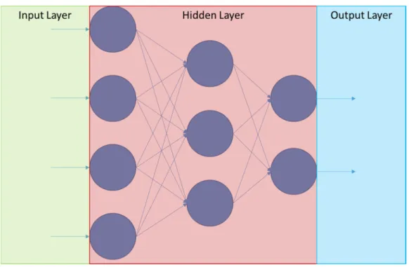
More complicated structures can be created using perceptrons as a building block. When multiple perceptrons are combined together in a layered structure with all edges moving in a single direction, a feedforward neural network or Artificial Neural Network (ANN) is created. These networks have a specific arrangement of layers, with the most common being a single input layer, multiple hidden layers, and a single output layer. ANNs are considered to be universal function approximators and can handle very complex problem with the addition of more nodes and layers.
Figure 4. Fully-connected artificial neural network
Each node in Figure 4 represents a perceptron with multiple inputs and multiple outputs. Calculations are performed from left to right with the numerical results flowing from the input to the output. This process can be understood at a macroscopic level as a set of input values being modified by the hidden layer to produce a desired result at the output layer.
Convolutional Neural Networks
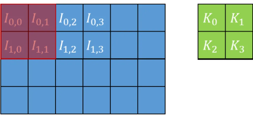
CNNs are a special type of ANN which is designed to leverage the spatial relationships of input data. These type of networks are commonly used for image classification, and are currently considered the state of the art approach for this task [7] [19]. CNNs implement several changes to the typical ANN architecture such as the use of the convolution, sparse connections, and weight sharing. The convolution function works by sliding a window across a multi-dimensional array of data. This window is referred to as the convolutional kernel. Each cell of this kernel has a parameter which is multiplied by the corresponding parameter in the input array. The products of each cell in the kernel window are then added together completing the convolution.
Figure 5. Visual representation of the convolution operation, with the kernel parameters in green, the window in red, and the input matrix in blue.
, ∗ , ,
(2)
,
Since the convolutional function rolls together all of the elements within the kernel window the interaction of these elements is preserved. The convolutional
operation also has several specified hyper-parameters, the first of which is the window size; Figure 5 shows a convolution with a window size of 2x2 elements. The other hyper-parameter is the stride of the convolution which controls how far the window is moved after each convolution, for example if the stride is two then the window will shift two elements over after each calculation. The stride of the convolution affects the size of the output array, as convolutional layers with larger stride need less steps to move across the entire array.
Supervised Learning
When neural networks are trained using labeled training data, it is called
supervised learning. When training a network using a supervised approach the goal is to learn a generalized function based on the training dataset. One particular consideration during the supervised learning process is the tradeoff between bias and variance. Bias is error that arises from poor restrictions imposed on the model; as an example when
attempting to fit a line to a non-linear function there would be high bias error. Variance is error that arises from a model that is too flexible and sensitive to specific characteristics of the data. The equation below shows that the total expected error of a model is made up of three separate error components: Variance, Bias, and irreducible error ϵ [20].
(3) Furthermore, high bias error causes a supervised network to under-fit the training data and not learn salient features of the data. High variance error causes the supervised network to over-fit the training data and not learn generalizable features. Finding the
proper balance between bias and variance through the use of larger networks and regularization techniques is the key to achieving optimal generalized network performance [21].
Regularization
Regularization is a collection of singular techniques which aim to reduce the amount of overfitting that occurs during the training process. Some commonly used regularization techniques include dropout [22], batch normalization [23], and transfer learning [24]. Each technique has pros and cons, and some techniques like dropout and transfer learning can be used simultaneously. The use of these techniques is particularly important when there is limited training data or a neural network is created with many layers. The number of layers a neural net has is proportional to the amount of capacity it has to approximate the desired function. Capacity however comes at a cost; too much capacity and the network will easily over fit the training data and perform poorly on general data. The use of regularization allows for the use of deeper networks while still preserving the generalized performance of the network. Dropout is the most commonly used of these techniques and it works by selectively disabling connections between nodes during a training epoch. This helps the network by forcing it to not rely too heavily on any given sequence of connections, thus making activations more general and robust. The amount of connections disabled between two layers is a hyper-parameter and values of around 15%-40% are common [22].
Activation Functions
The activation function is an important part of the perceptron as it allows for the modeling of non-linear functions by a neural network. Of the many choices for the activation function the two functions that see widespread use are the sigmoidal function and the ReLU function. Both the sigmoid and ReLU functions are shown in Figure 6.
Figure 6. Comparison of commonly used activation functions.
1
1 , max 0, (4)
Recently the ReLU has overtaken the sigmoid as the activation function of choice for deep neural networks due to its ability to better handle vanishing gradients, its
reduced computational complexity, and finally its ability to maintain information through many layers.
III. Methodology
Exploration of this research area was pursued in a progressive fashion that can be broken down into iterative three phases. The first phase is the collection and creation of the dataset from satellite images using automated coordinate based techniques. This results in nearly automated dataset generation which leverages the geospatial metadata on RS imagery. The second phase is a limited exploration of the generated dataset and hardware/software setup, which culminated in the testing of primarily grayscale networks. The testing conducted in the second phase was restricted by software constraints and a limited preliminary dataset. The third phase is where the primary experimentation took place. In this phase all restrictions imposed on the first round of testing were eliminated and a much larger dataset was used. The testing consisted of the selection and training of multi-color networks on a more efficient CNN architecture. Datasets
Prior to selecting Landsat-8 as a raw imagery source and processing it into a dataset, several pre-existing datasets were investigated for their applicability to this area of research. The following sections describe these datasets and indicates why they were ultimately not suitable for this research. The SAT-4 [25], SAT-6 [25], NLCD 2006 [26], ISPRS Vaihingen [27], ISPRS Potsdam [28], and SpaceNet datasets were all evaluated for use. Finding the right combination of full earth coverage combined with the presence of many multi-spectral bands was challenging and none of the existing datasets fully satisfied the specific needs of the research objectives.
SAT-4 & SAT-6 Datasets
The SAT-4 and SAT-6 datasets consist of data collected from the National Agriculture Imagery Program (NAIP). The imagery contained has four bands; the standard red, green, blue visible bands and one NIR band. The SAT-4 and SAT-6 datasets contain an
impressive 500k and 405k cropped image patches respectively. However the labeled classes are general land biomes, with the SAT-4 dataset having 4 categories: barren land, trees, grassland, and all other land. The SAT-6 dataset is similar to the SAT-4 dataset with two new classes added that cover human development: roads and buildings. Both datasets are broken down into 28 x 28 image patches or tiles [25]. Use of this dataset for training an airport detector is not feasible. Several issues arise, the first being that the 28 x 28 tile size doesn’t mesh well with most pre-developed ImageNet based networks. This means that no transfer learning can be leveraged when training a network due to the standard ImageNet size being around 256 x 256 pixel tiles. The second issue with this dataset is that the categories don’t mesh well with detecting any specific target. While the SAT-6 dataset contains both roads and buildings generally, it doesn’t specify any useful notional targets. The third drawback is that this dataset only has 4 bands for use, which would limit the amount of multi-spectral analysis that could be done. The inclusion of a NIR would allow for some limited experimentation to be conducted.
National Land Cover Database
The National Land Cover Database (NLCD) 2006 dataset covers the entire continental United States using Landsat-7 imagery with a pixel resolution of 30m/pixel. Land is classified into one of 16 development and/or Biome categories. While the source imagery has many bands due to its Landsat-7 source [29] it doesn’t label structures, but
instead categorizes large tracts of land. Due to the nature of the labeling this dataset was deemed to not be appropriate for training a notional airport target detector.
ISPRS Valihingen & Potsdam Datasets
The International Society for Photogrammetry and Remote Sensing (ISPRS) Valihingen [27] and Potsdam [28] datasets contain semantically labeled imagery. The scope of each dataset is limited to its respective city, with the Vaihingen dataset having 33 patches of labeled data and the Potsdam dataset having 38 patches of labeled data. The images come in several formats consisting of false color images, visible, and visible plus Infrared. In total there are four color bands for every patch. The limited size of these datasets made it a bad fit for global classification of targets. Additionally this dataset was designed to be used when training a semantic segmentation network which assigns a class to each pixel within an image instead of classifying the overall image. This differs from the classification of the entire image and then localization approach that is taken for this research, causing these datasets to not be suitable.
SpaceNet Dataset
The SpaceNet dataset is a relatively new data source and was the last dataset considered for use. SpaceNet was created using DigitalGlobe imagery from the Worldview-3 satellite, and includes truth data for several selected Areas of Interest (AOIs). Currently the following cities are included in the dataset: Rio de Janeiro, Paris, Las Vegas, Shanghai, and Khartoum. Truth data for each city consists of road and building footprints for all cities, and marked Points of Interest (POIs) for Rio de Janeiro. Images are up to 30cm in resolution depending on the sensor band, with up to 8-band multispectral available. While the SpaceNet dataset offers best in class resolution and
multiple spectral bands, it still has limited AOI’s for training and limited target types to train a network on. Due to the limited number of AOI’s and target types this dataset was ultimately not utilized.
Automated Dataset Generation
After exploring existing public datasets it became clear that all options would present restrictions to the research. Instead the chosen approach was to create a new RS dataset from minimally processed imagery combined with geospatial metadata. The strategy in creating this dataset was to avoid the typical approach of hand labeling a small amount of images. Instead a new approach was devised which leverages coordinates as the source of truth information.
Almost all commercially available satellite imagery includes geospatial metadata which correlates the pixels of the image with a location on the earth’s surface. The most common image format which includes this metadata is the GEOTIFF format; geospatial information is contained within headers. From a dataset creation aspect this information presents an opportunity to correlate coordinates with pixels within a given image. Coordinate lists exist for many targets of interest and the pixels of these targets can be found within images using only coordinate information and no further human input.
The pipeline for creating a new dataset using coordinates is shown in Figure 7. This approach was developed using the publicly available Landsat-8 data as an example, but the methodology applies to any collection of GEOTIFF images. The entire process uses only two csv files as an input; the first file is a listing of the target coordinates, and the second file is a listing of the available imagery. The first file contains information about individual targets on each row, including the latitude and longitude coordinates of
each target on the earth. Additional information like the name of a target and other classifying information can also be recorded. The second file contains a listing of all available Landsat-8 scenes in a Bounding Box (BBOX) format. This format indicates the latitude and longitude corner coordinates for each image contained in the listing. Image acquisition time, pre-processing information, cloud cover, and the download URL are also included in the Landsat metadata file.
Figure 7. Overview of Automated Dataset Generation Pipeline
The two input files are used in conjunction to perform a search for Landsat scenes which contain targets. The search is flexible enough to handle multiple classes and multiple targets in a single scene. Additionally, when searching, a cloud cover threshold can be specified which will limit the search results to only images with an estimated cloud cover at or below the threshold. Cloud cover estimates are provided in the Landsat metadata file and are created from the Band-9 images. Band 9 is the Cirrus cloud band and the wavelength was chosen to respond well to cloud cover in an image. The output of the search algorithm is a new csv of scenes which contain targets. Information for
multiple targets is concatenated together for use later in the pipeline. An excerpt from the found targets csv is shown below in Figure 8.
Figure 8. Excerpt of rows from found targets CSV
One drawback of the bounding box search method is that a subset of the found scenes don’t actually contain targets. This is due to the orientation of Landsat-8 images which are rotated and inscribed within a box. This leads to four triangular areas at the edges of the image which are completely black and contain no information. Removing targets which fall into these areas is solved later in the pipeline with a simple darkness check. Figure 9 shows the erroneous regions described above.
Once the found scene list is generated the next step of the pipeline is to use the provided hyperlinks to download the raw Landsat-8 images. The structure of the hosted database does not support the acquisition of scenes at the scale that AI research
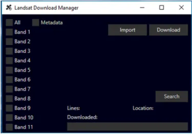
necessitates. To resolve this issue a program was written to handle the batch downloading of Landsat-8 scenes. The selection of which bands to download is available through a GUI and the scenes to download are indicated in the found scenes list.
Figure 10. Imagery Download Manager
After the scene downloading phase is over the next step is to turn the raw image into truth labeled tiles. This is accomplished by using the raw Landsat scenes and the original list of target coordinates. The location of any given target is pinpointed within an image by converting the latitude and longitude coordinates into a pixel location. This is accomplished using the Geospatial Data Abstraction Library (GDAL) and results in better precision that a simple percentage offset.
∗ ∗
∗ ∗ (5)
, &
Using the coordinate to pixel conversions in the GDAL library [30], the center-point of the target can be easily found and an area surrounding the center-center-point can be extracted as a tile. The area of the tile is specified within the program and a nominal size of 256 x 256 was chosen to conform to the historical ImageNet [31] standard. Since the class of each target is annotated in the previous steps, the resulting tile from cropping any given target is also able to be labeled with no further effort. Therefore the tiling algorithm not only creates the dataset images, but also labels them with the truth marking in a single step. Targets themselves are mapped to directly with other parts of the image being tiled as well. The purpose of tiling other portions of the raw image is to create an additional class of background scenery for network training. The background class consists of everything other than the selected targets.
Two different tiling schemes were developed for generating the scenery class tiles. Both approaches share the key features of image and tile boundary preservation. This means that the target and scenery tiles respect the boundaries of the source Landsat-8 image, as well as the scenery tiles additionally respecting the boundaries of the target tiles. This is a very important feature because it prevents the partial inclusion of target tile pixels in other target classes or the scenery tiles. Another shared capability between both schemes is the ability to crop multiple targets and multiple target types simultaneously.
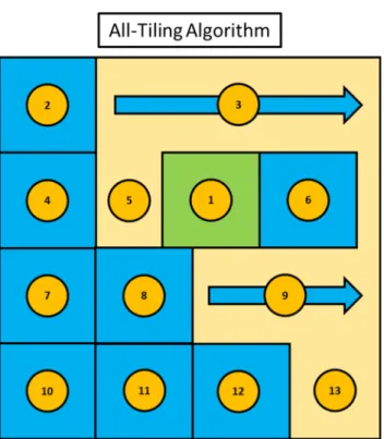
Method one or the “All-Tiling algorithm” attempts to create the maximum amount of tiles from a source image, while still respecting the boundary rules described previously. An average Landsat-8 scene yields between 900 & 1000 tiles, with 1-6 target
tiles and 900+ scenery tiles. The algorithm is shown visually for an example scenario in Figure 11.
Figure 11. Landsat-8 scene tiled using the All-Tiling Algorithm. Green tiles represent targets & blue tiles represent background scenery
The All-Tiling algorithm starts by first creating tiles for all of the targets in every indicated target class. After generating the target tiles the tile bounds are recorded and referenced during the creation of the scenery tiles. Scenery tile generation starts in the upper left corner of the source image and moves across the image to the right. As tiles are created their bounds are checked against the previously created target tiles and the image bounds. If a candidate tile violates either of these bounds it is not generated and the algorithm skips ahead to the next valid tile. In Figure 11 marker five shows how the algorithm tiles around a target tile, and marker thirteen shows how the algorithm stops creating tiles at the edge of the image.
Method two or the “Adjacent-Tiling algorithm” takes a different approach to tiling the source image. Instead of maximizing the number of generated tiles, it only creates scenery tiles that are touching target tiles. A maximum of 8 scenery tiles are generated for every unique target tile. This leads to a much smaller amount of total tiles generated with the same average of 1-6 target tiles, and a more limited 8-48 scenery tiles.
Figure 12. Landsat-8 scene tiled using the Adjacent-Tiling Algorithm. Green tiles represent targets & blue tiles represent background scenery
The Adjacent-Tiling algorithm begins by all of the target tiles first, followed by the generation of the scenery tiles. Following the creation of all target tiles the scenery tile generation start at to the upper left of a given target tile. The first scenery tile is offset by one tile length in the X dimension and one tile length in the Y dimension. The
algorithm then proceeds to crop around the target tile in a clockwise fashion until it arrives at the upper left location. Marker’s eight, nine, and ten show a situation where
scenery tiles are skipped to avoid duplication and to respect the boundary of the original image.
Enhancements were made to the auto-tiling algorithms to speed up the dataset creation time. Initial estimates projected that the time required to tile all 315,000 potential Landsat images was between 15 and 20 days. While this timeframe was achievable, it represented a huge bottleneck for dataset creation. Parallelization of the auto-tiling code was pursued to dramatically reduce the time required for processing images. This was possible because the tiling of any given image is completely independent, which allows for processing multiple images simultaneously.
Figure 13. Tiling speedup using multi-processing, darkened points indicate that the number of threads and cores are equal
Table 4. Hardware test configuration for parallel speed characterization Hardware Configuration Operating System Ubuntu 16.04 GPU #1 Tesla K40 GPU #2 Quadro M6000 RAM 256 GB SSD 256 GB HDD 4 TB 7200 RPM Processor 2 x 14 Core Intel
Figure 13 shows the results of testing the relationship between program speed and the number of CPU cores utilized. Testing was carried out using both HDDs and SSDs, and across 1 to 40 threads. Dark points on the graph indicate where the number of CPU cores equals the number of threads. Optimal performance also occurs at this point, which for the test system is 28 cores. HDD performance is better when the number of threads is less than 12, after which point the SSD begins to perform faster. The fastest throughput recorded for Landsat images was 160 scenes/minute, generating approximately 160k tiles/minute. This translates into nearly 360 hours saved when tiling the entire Landsat dataset.
The output of the auto-tiling algorithms are tiles separated by their class labels. At this stage the total collection of tiles can be split up into training, validation, and test subsets as needed. When generating datasets particular consideration was taken to address the imbalance of tiles between classes. Class imbalance arises from the behavior of the backpropagation algorithm, which rewards or punishes network weights based on the batch classification accuracy during training. If you have many examples of a single class then there will be a proportional amount of weights updated based on this class, which causes the network to perform better on that class. In a multi-class problem,
maximizing the classification accuracy of a single class may lead to lower accuracy on all classes with less training examples and ultimately lower overall classification accuracy. Depending on which tiling algorithm is used, there can be over a 100:1 ratio between target and scenery tiles. Two options were considered to deal with the imbalance [32]: adjust the backpropagation algorithm during training or sample from the scenery tiles.
One method of dealing with class imbalance is to normalize the effect that tiles from each class have on the backpropagation algorithm. For the situation described previously this would consist of reducing the effect that scenery tiles have during training to compensate for the increased number of these tiles. The alternative method is to
randomly sample from all of the available scenery tiles, which ensures that there are an equal number of target and scenery tiles in the dataset.
Finally the last step of the dataset generation pipeline is to create a dictionary listing with the tile locations in memory and the class labels. This dictionary file is used during the training process to generate batches of tiles for the neural network.
Figure 14. Sample results from Auto-Tiling algorithm. A full size Landsat-8 image is shown in top left, with four resulting tiles shown on the right. A typical
Landsat-8 scene yields over 900 individual tiles. Images courtesy of the U.S. Geological Survey. First Experiment Methodology
For the experimental portion of this research two separate experiments were planned. The first experiment was conducted largely as a proof of concept, with the goal
of validating the notional target selection, imagery source, and automated dataset
generation. Several restrictions were placed on this experiment because at the time only a limited dataset was available and default imaging libraries were used for handling data batches for training. Large airports were the only target class considered in this
experiment, which led to the number of images in the dataset to be limited. The
experiment was also restricted to using networks trained on either single color images or composite RGB images. Finally the color bands were also restricted to only bands with the same pixel resolution of 30m/px (B2-B7). The panchromatic band was the only band not considered since it has double the pixel resolution of all other bands.
Table 5. Dataset for experiment #1 broken down by selected processing stages Experiment #1 Dataset
CSV Files 567 Large Airports
Found Airports 2500 scenes x 6 Bands Generated Tiles 900 – 1000 per scene
Airport Tiles 1007 x 6 Bands
Non Airport Tiles 1007 x 6 Bands
Total Tiles 12,084 Tiles
The dataset used for experiment one is shown above in Table 5, starting with a list of 567 large airports 1007 tiles were generated. An additional 1007 non-airports or
scenery tiles were also sampled from the available pool of tiles. The same 2014 target and scenery tiles were collected across B2-B7, resulting in a total of 12,084 tiles for the entire dataset. The total dataset was split into smaller training and testing subsets. A validation set was not created for this experiment because no hyper-parameter tuning or early stopping was used. Preservation of the test set data was maintained by not applying any tuning decisions to it as well. Training and testing size was determined by using a 70%
training and 30% testing split, resulting in a training dataset of 8,388 tiles and a test dataset of 3,696 tiles.
Several network architectures were explored for the first CNN with the ultimate choice being the VGG-19 [5] architecture. The following network architectures were considered: AlexNet [4], VGG-16, VGG-19, ResNet [34], GoogleNet [33], and
SqueezeNet [6]. Most of these architecture were developed in response to the ImageNet challenge (ILSVRC) [31], and were at the time of their introduction leading architectures in terms of Top-1 and Top-5 accuracy in the 1000 class problem. Each architecture also leverages the spatial relationships of pixels using convolutional layers in some fashion, leading them to all be considered types of CNNs.
AlexNet
AlexNet was the CNN that started the modern deep learning revolution and at its time it shattered the existing record in the ILSVRC competition. The network introduced a number of key features which when utilized together led to the record breaking
accuracy. The architecture consisted of 5 convolutional layers followed by 3 fully connected layers and then finally a 1000-class softmax layer for the output. The network also used Rectified Linear Unit’s (ReLUs) for the activation function, Dropout layers to increase regularization, and optimized GPU training. AlexNet was the best performing network in the ILSVRC-2012 competition with a Top-5 test accuracy of 15.3%.
VGG-16 & VGG-19
The Visual Geometry Group (VGG) 16 & 19 architectures represent the natural progression of deep CNNs inspired by AlexNet. The architecture was developed by the Visual Geometry Group at the University of Oxford in 2014. It consists of a deeper
architecture than previous ILSVRC submissions with 16 layers and 19 layers
respectively. Increased depth was made possible by reducing the size of the convolutional filters from 11x11 or 7x7 down to 3x3 pixels. The stride of the window is also reduced from either a 4 pixel or 2 pixel stride to the smallest possible 1 pixel stride. VGG architectures also utilize the ReLU activation function for its computational efficiency. With this deeper architecture a very high Top-5 test accuracy of 7.3% was achieved in the ILSVRC-2014 competition. The VGG architecture still sees common use due to its intuitive design and respectable performance.
GoogleNet
The GoogLeNet architecture represents one of the first departures from the paradigm of simply adding more layers. It introduces an entirely new type of architecture building block called an inception module. Through the use of these inceptions modules the architecture is able to increase the width and depth of the network without increases the overall computational load. The final network design employs 22 layers, uses ReLU activation, and has 12x less parameters than AlexNet while also having increased performance. The inception modules themselves consist of a collection of possible layer types including 1x1 conv, 3x3 conv, 5x5 conv, and max pooling. During training the selection of layer type is not pre-defined allowing the network to optimize for the proper inception module subset. Designed with computational efficiency in mind the
architecture still logged a Top-5 test error rate of 6.67% in the ILSVRC-2014 competition.
ResNet-152
ResNet-152 is a network architecture developed by Microsoft research for the ILSVRC-2015 competition. It features an incredible 152 layer architecture, which was and still is vastly deeper than any other architecture proposed. Despite the increased number of layers, the complexity of the network is actual lower than AlexNet or VGG. One major innovation of this network is the addition of skip connections from lower layers to deeper layers to combat the vanishing gradient problem [35]. An ensemble of ResNet-152 networks achieved a Top-5 test error rate of 3.57% in the ILSVRC-2015 competition.
SqueezeNet
Finally the last network architecture considered was the SqueezeNet architecture. SqueezeNet aims to reduce the size of the overall network rather than pursue pure
performance. This sets it apart from many of the other architectures already discussed and causes the network to have many advantages that make it an attractive choice. Some of the advantages of SqueezeNet are reduced server communication during training, less bandwidth to move trained networks to a deployed system, and the feasibility to deploy the network on memory limited devices like FPGAs. Size reductions are achieved
through the use of the fire module, which uses a squeeze and expand design. The squeeze is achieved by using a simple 1x1 convolution layer and the expansion is achieved by following up with both a 1x1 convolution and 3x3 convolution in parallel. These outputs are concatenated and passed to the next layer. The magnitude of size reductions is
parameters. Further reductions in size of up to 510x can be achieved using model compression techniques.
Custom VGG-19 Network
Figure 15. Modified VGG-19 architecture used in experiment one. After considering all of the network architectures discussed above, a modified version of the VGG-19 [5] architecture was chosen. VGG-19 was chosen because of its simple design and high accuracy. The modifications made to the network are shown in Figure 15; all convolutional and max pooling layers were preserved with the fully connected layer modified to better accommodate a 2-class problem. The fully connected layers were reduced in width from 2048 to 1024 nodes each, with the output layer reduced to a 2-class softmax.
For all tests the modified VGG-19 network was pre-trained using ImageNet weights. Transfer learning was employed for this experiment for a few reasons, the first
reason was that the limited dataset could benefit from the much larger ImageNet dataset. The second reason was that since only grayscale and 3-color RGB networks were being tested, it opened up the possibility of ImageNet weights. If networks were tested using more or less than 3-colors there would be no way to correlate the ImageNet weights, which were developed using only RGB images. The pre-trained VGG-19 architecture’s input layer contains one weight value for each pixel and each color, this results in 3 different weights for every pixel representing the pathway from red, green, and blue. Combinations of these weights between colors and between pixels occurs in subsequent convolutional layers. When feeding new data through this pre-trained network the mapping of training image colors to existing color pathways needs to be maintained and the number of colors must be the same. If the number of channels in the input images changes then there would be no corresponding pathway in the network. To address this issue for single band or grayscale networks and benefit from ImageNet pre-training, the single colors were duplicated into all 3 color channels to create a false RGB image as shown in Figure 16 below.
Figure 16. False color images were created by duplicating pixels from a single band into the RGB color channels.
During the network training portion of the experiment certain layers of the network had their weight locked. The only layers that were allowed to be updated by the backpropagation algorithm were the fully connected layers. This meant that the feature extractions being outputted from the convolutional layers were unchanged from the ImageNet dataset. This decision was made again due to the limited amount of data
available for the first test. The rationale was that limited data could not have a meaningful effect on so many convolutional layers and could also overwhelm the weights already present from the ImageNet pre-training.
Second Experiment Methodology
The primary goal of the next experiment was to remove all of the restrictions imposed in the first experiment. The removal of those restrictions allowed this
experiment to answer several questions simultaneously. Next, since the Panchromatic Band-8 is twice the resolution of the other color bands, the effect of resolution on classification accuracy is also addressed. Another area of investigation was the strategy and benefit of combining many color bands to increase classification accuracy. Finally the experiment explored the use of an alternative architecture which has greater
parameter efficiency.
Table 6. Dataset for experiment #2 broken down by selected processing stages. Experiment #2 Dataset
CSV Files 5099 Large/Medium Airports Found Airports 9000 scenes x 7 Bands Generated Tiles 900 – 1000 per scene
Non Airport Tiles 9459 x 7 Bands
Total Tiles 132,426 Tiles
The dataset for experiment two is shown above in Table 6. This experiment expands the number of starting targets by including both large and medium airports. Both types of airports are consolidated into a single airport class, with the other class once again being the background scenery. Included in the dataset are tiles from Landsat-8 bands 2 through 8. Bands 2 through 7 have a pixel resolution of 30 meters and Band-8 has a resolution of 15 meters. Broken down by band the dataset contains 9,459 tiles in each class and over 130k tiles across all bands. The dataset was also split further in three subsets: training, validation, and test. The split between the three subsets was 70 percent training, 10 percent validation, and 20 percent test.
The training set contained 6,621 tiles from both the airport and scenery classes. This subset is the only data that the network is shown during the training and
backpropagation phase. The validation set consisted of 945 tiles per class, and is used for several different purposed during this experiment. The primary use of the validation set is for hyper-parameter tuning, such as selecting an appropriate learning rate and optimizer. It is also used for selecting an optimal stopping point during the training phase. Finally the validation set was also used for evaluating the similarity of the tiles in each color band. The last subset created is the test set which is used after training to determine the classification accuracy of the network.
For this experiment a new architecture was chosen with fewer parameters than the first experiment. The modified VGG-19 architecture was abandoned for two reasons; the first was that the network was originally designed for use on 1000-class problems and
this research problem includes only two classes. This huge reduction in classes should lead to a reduction in the complexity of features needed to discriminate between targets and scenery. A complexity reduction should furthermore translate into a reduction in network capacity. The second reason for utilizing SqueezeNet is the speed at which new models can be created and trained. From a random weight initialization SqueezeNet models were trained for 200 epochs in about one hour. This benefited the second
experiment by allowing multiple models to be trained and evaluated for each color in the same time that one VGG-19 model could be trained. Due to the large amount of samples from each color, statistical methods such as t-tests parzen windows were employed to evaluate the relative significance of results. In light of the two aforementioned reasons the SqueezeNet architecture was utilized. The design of this architecture is shown below in Figures 17 and 18.
Figure 18. Detailed view of Fire Module
Data collection started with the training of single band networks for all colors. Several networks were trained for each color and the mean classification accuracies were recorded for each network. In the course of training, some networks remain stuck at a local minimum of around 50% classification accuracy. This situation is caused by the initial weights that are randomly assigned prior to network training. When this happens the training for the network is cut short and the results are ignored when calculating the mean classification accuracies.
Following the single color network testing the experiment proceeded to multi-color networks. These networks were trained on images with anywhere from 2 to 6 multi-color channels. The selection of which colors to combine and in what order to combine them is an open research question. Two different methods were tested during the course of the
experiment. Both methods operate by adding colors greedily based on a calculated metric. This approach is a modified case of the more general set cover problem [35], where the goal of the algorithm is to find a collection of subsets whose union covers the entire desired set.
: ∅ | ∩ |
In this case the desired set to be covered is the total information contained across all of the spectral bands available. The subsets that can be chosen from are each of the color bands B2-B7, and two different metrics were devised to estimate the information contained within each band.
The first metric used was the mean classification accuracy from the single band testing. Colors with the highest single band classification accuracy were added until no colors remained. Another more refined metric quantified the similarity of the images in each band’s dataset. This correlation metric was calculated by comparing the pixels of each tile in the validation set against all other colors. The metric also took into account the single band classification accuracy to ensure that while the colors are dissimilar, they each carry useful information. The end result is the selection of colors which are the most dissimilar to the already selected colors.
, , (6) : , , : , : max (7) : min (8) &
Once again multiple runs were done for each type of network created and for each of the greedy algorithm metrics. From these runs the average classification accuracy was calculated for all networks.
IV. Analysis and Results Experiment One
The results from the 1st experiment are shown in Figure 19 and Table 8 below. The
training algorithm utilized a Stochastic Gradient Descent (SGD) optimizer [36] with a learning rate of 0.0001 and a momentum value of 0.9. Networks were generated for each color and trained for a full 60 epochs before stopping. Test metrics were then collected using the models generated after the 60 epoch cutoff.
Table 7. Experiment #1 Hyper-Parameters and Test Configuration Experiment #1 Hyper‐Parameters Architecture VGG‐19 Optimizer SGD with momentum of .9 Learning Rate 0.0001 Epochs 60 Batch Size 64 Dataset Size 12,084 Training Set 70% Test Set 30% Pre‐Training ImageNet Early Stopping None
During the training phase all networks were able to reach 100% training accuracy and validation accuracy peaked at around 95% within 40 epochs for most bands.
Classification accuracy on the test set was fairly uniform with Band 6 – SWIR #1 seeing the lowest accuracy of all bands. Band 6 also saw greater instability during the training phase, with its accuracy varying widely. The composite RGB band saw no benefit over the grayscale networks even though it contained 3x the data of the grayscale networks. One observed benefit of the additional colors was a more stable accuracy during training.
Table 8. Test classification accuracy at epoch 60 Experiment #1 Classification Accuracy
Band Accuracy B2 - Blue 95.8% B3 - Green 95.8% B4 - Red 96.8% B5 - NIR 96.3% B6 – SWIR #1 93.5% B7 – SWIR #2 96.1% Composite RGB 96.1%
The uniform performance of the networks across bands and the observed ineffectiveness of color in increasing accuracy were unexpected results. Overall the classification accuracy was very good and all networks were able to distinguish the large airports from scenery over 93% of the time. The equality in performance could be explained by several factors. The first is that all networks were pre-trained with the ImageNet dataset, which contains over a million images and this coupled with the large number of parameters in VGG-19 leaves little chance for this dataset to have an effect. In fact out of the box the ImageNet features worked very well at identifying the new large airport class. Furthermore since the backpropagation was locked to only the fully
connected layers, variation between networks was controlled even further. Another factor could be the dataset itself which contained only the largest airports and randomly
sampled background tiles. Since these airports are bigger, it is expected that they will have more distinctive features for the network to extract. The background or scenery tiles also contain statistically “easier tiles”, which is due to the fact that most of the earth is ocean or wilderness. When encountered with undeveloped areas a classification is likely very easy as open plains is very different that paved airport runways. If the scenery tiles were selected to only represent urban areas instead of a random sample then the
classification accuracy could fall. The ambivalence of the networks to color can also be attributed to these factors and as will be seen in experiment two, when medium airports are included color becomes more noticeably important.
Experiment Two
The second experiment used a different optimizer than the first because training accuracy could not progress past random odds with an SGD optimizer. Instead an RMSProp with a learning rate of 0.0001 was used. The experiment started by training grayscale networks for Bands 2 through 8 several times. Training was run for a full 200 epochs with the best weights being saved. Saved models were determined based on their validation accuracy at the end of each epoch. If a model outperformed a previous version it was saved, if not it was passed over. Training error and validation error were logged at each epoch and saved for later analysis. Following the conclusion of each training run the test set was used to collect classification accuracy against the two classes. Mean accuracy values were computed once all training runs were completed.
Table 9. Experiment #2 Hyper-Parameters and Test Configuration Experiment #2 Hyper‐Parameters Architecture SqueezeNet Optimizer RMSProp with decay of 1 Learning Rate 0.0001 Epochs 200 Batch Size 64 Dataset Size 132,426 Training Set 70% Validation Set 10% Test Set 20% Pre‐Training None Early Stopping Peak Validation Accuracy
Figure 20 shows the training and validation accuracy for four example runs. The blue lines are the training accuracy and the orange lines the validation accuracy. The networks selected are one visible band, one infrared band, one double resolution band, and one multi-color network. These training curves demonstrate the typical divergence between validation and training accuracy, which indicate that some overfitting is occurring. The multi-color networks tend to have more stability in their validation accuracy in comparison to the grayscale networks. Resolution however does not provide the same type of stability and exhibits wide swings in accuracy.
Figure 20. Training and validation accuracy over time for selected networks Results from experiment #2 are shown in Figures 21-22 and Tables 10-12. Figure 21 shows the validation accuracy during training for all networks. In total this was 7 grayscale networks and 5 multi-color networks. The multi-color networks in Figure 21 were created using the greedy classification accuracy method. One interesting feature of